Relativistic Parker winds with variable effective polytropic index

Spherically symmetric hydrodynamical outflows accelerated thermally in the vicinity of a compact object are studied by generalizing an equation of state with a variable effective polytropic index, appropriate to describe relativistic temperatures close to the central object and nonrelativistic ones further away. Relativistic effects introduced by the Schwarzschild metric and the presence of relativistic temperatures in the corona are compared with previous results for a constant effective polytropic index and also with results of the classical wind theory. By a parametric study of the polytropic index and the location of the sonic transition it is found that space time curvature and relativistic temperatures tend to increase the efficiency of thermal driving in accelerating the outflow. Thus conversely to the classical Parker wind, the outflow is accelerated even for polytropic indices higher than $3/2$. The results of this simple but fully relativistic extension of the polytropic equation of state may be useful in simulations of outflows from hot coronae in black hole magnetospheres.

1 Introduction

Relativistic outflows are commonly inferred from observations of collimated winds (jets) in Galactic x-ray binaries and supermassive black holes in active galactic nuclei and quasars (Biretta et al. (1999); Livio 2002). Also, observations infer coronae with rather high temperatures in microquasars (e.g., Corbel et al. (2003)) and AGN (e.g., Rózańska & Czerny (2000) and refs. therein). Although there are still some ambiguities in the interpretation of these observations, usually temperatures up to $10^{9}$K for electrons/positrons and $10^{12}$K for protons are usually inferred. Nevertheless, even if such temperatures were to correspond to closed field line regions, by using the analogy with the solar corona, one may extrapolate that such high temperatures could also exist in the open field line regions where the outflow is accelerated. The heating mechanism to obtain these high temperatures can be of magnetic origin (Heinz & Begelman (2000)). Alternatively, accreted material falling onto the central black hole may be decelerated via a shock, feeding the magnetosphere with a hot plasma. Discussions on the possibility of such shock formation in an accretion disk that leads to a heated corona have been already given in the literature in the so called CENBOL model (Chakrabarti et al. (1996), Chattopadhyay et al. (2004), Das, 2000, and references therein). These papers have also discussed how radiation and coupling with the photon distribution has to be taken into account properly.

The inevitable result of such hot atmospheres is that they expand supersonically and at large distances thermal energy is converted to bulk flow kinetic energy. For example, Ferrari et al. (1985), Das (2000) and Chattopadhyay et al. (2004) have suggested that outflows can be thermally accelerated to relativistic speeds. However, such treatments assumed the classical polytropic equation of state which prevents from studying consistently the relativistic temperatures in the corona and the nonrelativistic ones farther away. The first effort to use an equation of state appropriate for outflows containing both ultrarelativistic and classical temperatures has been used only for studying spherical accretion flows and only in the adiabatic case (Mathews (1971); Blumenthal & Mathews (1976)). Moreover, Blumenthal & Mathews (1976) discussed the topology of the Mach number variation in the solution of an adiabatic wind.

However, as it is well known (Parker (1960)) the topology of the Mach number does not give us information on whether the flow itself is accelerated or not.

In this paper we extend the equation of state used in Blumenthal & Mathews (1976) for nonadiabatic flows and our goal is to investigate the efficiency of thermal driving under extreme relativistic conditions. For example, in the classical polytropic solar wind theory, the polytropic index needs to be smaller than $3/2$ in order to obtain an accelerated wind solution (Parker (1960)). This means that a minimal extension of the corona is required. Here we explore how this value is changed under relativistic conditions. In order to simplify the study, we shall focus our attention on spherical, steady and radial hydrodynamic outflows at large distances from a stationary compact object. Also for simplicity we shall use Schwarzschild’s metric.

Furthermore, we will not discuss how the pressure and the heating may include coupling with the radiation field, especially in the case of pair production, as our goal is to keep the discussion at a basic level and this has already been done elsewhere (e.g., Chattopadhyay et al. (2004)).

In the next section we outline the governing equations with particular emphasis to an equation of state appropriate to relativistic temperatures close to the base of the outflow and classical ones further away. In Sec. 3 we derive for a given asymptotic value of the polytropic index the range of allowed locations of the sonic surface and also the limits of the asymptotic speed. In Sec. 4 via a parametric study we present a comparison of our model with the nonrelativistic Parker wind and relativistic winds with constant polytropic index. An astrophysical application is outlined in Sec. 5 and the results are summarized in Sec. 6.

2 Basic Equations

The flow of a relativistic fluid is governed by conservation of the number of particles and energy-momentum,

$$(nu^{a})_{;a}=0\,,$$ (1)

$$(T^{ab})_{;b}=0\quad{\rm with}\quad T^{ab}=(nw/c^{2})u^{a}u^{b}+Pg^{ab}\,,$$ (2)

where $n$ is the proper number density of particles (electrons/protons, or, electrons/positrons) in the comoving frame of the fluid and $u^{a}=(\gamma c;\gamma\@vec{v})$ is the fluid four-velocity, with $\@vec{v}$ the spatial velocity and $\gamma=\left(1-{v}^{2}/c^{2}\right)^{-1/2}$ the Lorentz factor.

The proper enthalpy per particle, $w$, is the sum of the proper internal energy per particle (including the proper mass), $e$, and the proper pressure $P$ divided by $n$,

$$w=e+\frac{P}{n}\,.$$ (3)

The space-time around the central compact object is described by using Schwarzschild’s metric wherein in order to treat analytically the fluid equations the simplest way is to express all quantities in a 3+1 split space-time,

$${d}s^{2}=-\alpha^{2}c^{2}{d}t^{2}+\frac{1}{\alpha^{2}}{d}r^{2}+r^{2}{d}\theta^{2}+r^{2}\sin{\theta}^{2}{d}\phi^{2}\,,$$ (4)

where

$$\alpha=\sqrt{1-\frac{2{\cal G}{\cal M}_{\star}}{c^{2}r}}=\sqrt{1-\frac{r_{\rm G}}{r}}\,,$$ (5)

is the lapse or redshift factor induced by gravity at a distance $r$ from the central object (e.g., a black hole) of mass ${\cal M}_{\star}$, written also in terms of the Schwarzschild or gravitational radius $r_{\rm G}$,

$$r_{\rm G}=\frac{2{\cal G}{\cal M}_{\star}}{c^{2}}\,.$$ (6)

Assuming spherical symmetry such that the velocity is purely radial, $\@vec{v}=v\hat{r}$, Euler’s equation reduces to the following single differential equation,

$$\frac{1}{2}\gamma^{2}n\frac{w}{c^{2}}\frac{{d}{v}^{2}}{{d}r}+n\frac{w}{c^{2}}c^{2}\frac{{d}\ln\alpha}{{d}r}+\frac{{d}P}{{d}r}=0\,.$$ (7)

By combining Eqs. (2) and (3), we get that the variations of the specific enthalpy and internal energy are

$${d}w=\frac{1}{n}{d}P\,,\quad{d}e=\frac{P}{n^{2}}{d}n\,.$$ (8)

Similarly, the conservation of the number of particles for a spherical wind, Eq. (1), takes the following simpler form,

$$\frac{d}{{d}r}(\alpha\gamma nvr^{2})=0\,.$$ (9)

In the following, we shall adopt an equation of state appropriate to describe relativistic temperatures close to the central object and nonrelativistic ones further away and also derive its ultrarelativistic and classical limits.

2.1 Closure of the fluid equations

To close the system of equations, (7-9) we should specify an equation of state that relates the entropy per particle $s=s(w,P)=s(e,P)$ to the pressure, $P$, and the enthalpy per particle, $w$, or the internal energy per particle, $e$. In the literature (e.g., Michel (1972); Chakrabarti et al. (1996); Das (1999)) various authors have adopted a classical adiabatic or polytropic equation to replace the equation of state

$$P\propto n^{\Gamma}\,,$$ (10)

where $\Gamma$ is a constant. However, in this form $\Gamma$ should attain different values whether the particles are in a relativistic or a classical thermodynamical regime. It is well known that for a monoatomic gas, in adiabatic flow the index is $5/3$ in the classical regime with nonrelativistic temperatures ($k_{\rm B}T\ll mc^{2}$), and $4/3$ in the ultra-relativistic one ($k_{\rm B}T\gg mc^{2}$). (Here $k_{\rm B}$ is the Boltzmann constant and $mc^{2}$ is the rest mass energy per particle.) Thus we can define an effective polytropic index

$$\Gamma_{\rm eff}=\frac{{d}\ln{P}}{{d}\ln{n}}$$ (11)

which should vary with temperature. In other words, the previous equation of state with a constant index cannot account for media with a transition from ultrarelativistic to nonrelativistic temperatures, as inferred from observations of coronae in AGNs.

The scalar isotropic pressure of a single perfect fluid is given by (Mathews (1971); Synge (1957))

$$P=\frac{1}{3}n\epsilon_{0}\left(\frac{e}{\epsilon_{0}}-\frac{\epsilon_{0}}{e}\right)\,,$$ (12)

where $\epsilon_{0}=mc^{2}$. Its validity for collisional and collisionless fluids is discussed in detail in Blumenthal & Mathews (1976) and we refer the reader to section III of their paper.

By integrating Eqs. (8) and (12) we obtain a generalized equation of state for an adiabatic (ideal) fluid (see Blumenthal & Mathews (1976), Eq. 3.3),

$$e^{2}-\epsilon_{0}^{2}=\kappa n^{\frac{2}{3}}=\kappa n^{\Gamma_{\rm ad}-1}\,,$$ (13)

which represents the equation of state for an adiabatic flow. Here $\Gamma_{\rm ad}=5/3$ is the real adiabatic index related to the number of degrees of freedom of the particles.

For studying stellar interiors, a classical trick to study different equations of state and their hardness is to use the same equation, called polytropic equation of state, with a different value of the adiabatic index, assuming the number of degrees of freedom of the particles has changed. In this case $\Gamma_{\rm ad}\neq 5/3$, but the system still evolves adiabatically. E. Parker to study the solar wind proposed (Parker (1960)) to follow the same path using Eq. 10, assuming $\Gamma$ being any value between 1 and the adiabatic value $5/3$ to mimic the coronal heating in a simple but hidden way. As explained in Sauty et al. (1999) this is equivalent to use a generalized enthalpy and internal energy which includes the heating.

Following Parker’s initial approach of the polytropic solar wind, we assume also here that the enthalpy and the particle density are related by Eq. (8) but relating $e$ to the particle density via

$$e^{2}-\epsilon_{0}^{2}=\kappa n^{\Gamma-1}\,,$$ (14)

with again a value of the constant polytropic index $\Gamma$ which can be anything between 1 (isothermal) and 5/3 (adiabatic value), or higher in case of energy losses. The basic idea is to generalize to heated relativistic winds the approach of Blumenthal & Mathews (1976) for relativistic accretion flows like Parker did with Bondi’s accretion models. Of course at this stage $w$ (resp. $e$) is a generalized specific enthalpy (resp. generalized specific internal energy) which includes the energy brought via heating from the external medium. We recall in Appendix A how to calculate the extra heating implicitly in the case of a monoatomic ionized plasma.

By combining Eq. (14) and (8) we get a generalized relation between pressure and density which includes the proper mass energy per particle, $\epsilon_{0}=mc^{2}$ ,

$$P=\frac{\Gamma-1}{2}\frac{\kappa n^{\Gamma}}{\sqrt{\epsilon_{0}^{2}+\kappa n^{\Gamma-1}}}$$ (15)

for $\Gamma\neq 1$. Note that Eq. (15) is a generalization of the usual form of the so-called equation of state with the inclusion of relativistic thermal effects. Thus the effective polytropic index (Eq. 11) takes the form

$$\Gamma_{\rm eff}=\Gamma-\frac{\Gamma-1}{2}\frac{\rho}{1+\rho}\,,$$ (16)

where we have introduced a new dimensionless function $\rho$

$$\rho=\frac{e^{2}-\epsilon_{0}^{2}}{\epsilon_{0}^{2}}=\frac{\kappa n^{\Gamma-1}}{\epsilon_{0}^{2}}\,.$$ (17)

All thermal effects appear in this single function $\rho$, hence decreasing the number of free parameters in the model.

Finally, the local sound speed $v_{s}=\beta_{\rm s}c$ can be written as a function of $\rho$,

$$\beta_{\rm s}^{2} \;=\; \frac{v_{\rm s}^{2}}{c^{2}}=\frac{1}{w}\frac{{d}P}{{d}n}\,$$ (18)

$$\;=\; \frac{\Gamma-1}{2}\left\{1-\frac{2+(3-\Gamma)\rho}{(1+\rho)[2+(\Gamma+1)\rho]}\right\}\,.$$

The logarithmic derivative of the sound speed with density is

$$\frac{d\ln\beta_{\rm s}^{2}}{d\ln\rho}=\frac{(\Gamma+1)(3-\Gamma)\rho^{2}+4(\Gamma+1)\rho+4\Gamma}{(\rho+1)\left[2\Gamma+(\Gamma+1)\rho\right]\left[2+(\Gamma+1)\rho\right]}\,,$$ (19)

and, for $\Gamma<3$, it is positive. Thus, with $\Gamma<3$ it follows that

$$\beta_{\rm s}^{2}\leq\frac{\Gamma-1}{2}\,,$$ (20)

with the equality holding in the high temperature limit ($\rho\longrightarrow\infty$). Note that for $\Gamma<5/3$, we get the usual condition $\beta_{\rm s}^{2}<1/3$ (Michel (1972)).

2.2 Nonrelativistic and ultrarelativistic limits

In the limit of a nonrelativistic fluid, $\epsilon_{\rm th}\ll\epsilon_{0}$, we may calculate the thermal energy per particle or random thermal energy (Mathews (1971)),

$$\epsilon_{\rm th} =e-\epsilon_{0}=\sqrt{\kappa n^{\Gamma-1}+\epsilon_{0}^{2}}-\epsilon_{0}$$ (21)

$$\approx\frac{\displaystyle\kappa}{\displaystyle 2\epsilon_{0}}n^{\Gamma-1}{{\rm,\qquad\qquad if\ }\epsilon_{\rm th}\ll\epsilon_{0}}\,.$$

In such a case, $\rho$ is twice the ratio of the thermal energy per particle and the mass energy

$$\rho\approx 2\frac{\epsilon_{\rm th}}{\epsilon_{0}}\,.$$ (22)

For classical temperatures, wherein the thermal energy is negligible compared to the mass energy, $\epsilon_{\rm th}\ll\epsilon_{0}$, we have that $\rho\ll 1$ and

$$P\simeq\left(\Gamma-1\right)n\epsilon_{\rm th}\simeq\;\left(\Gamma-1\right)\frac{\kappa}{2\epsilon_{0}}n^{\Gamma}\,,$$ (23)

such that the effective polytropic index is exactly $\Gamma_{\rm eff}=\Gamma$. In general, as temperature decreases with distance, $\Gamma$ always represents the asymptotic value of the effective polytropic index. This allows us to have a simple albeit artificial way to model relativistic coronae as in the classical Parker wind.

On the other hand, in the ultrarelativistic domain where the thermal energy is much larger than the mass energy ($\epsilon_{\rm th}\gg\epsilon_{0}$ $\Leftrightarrow$ $\rho\gg 1$) we have

$$P\simeq\frac{\Gamma-1}{2}{\kappa^{\frac{1}{2}}n^{\frac{\Gamma+1}{2}}}\,.$$ (24)

The effective polytropic index becomes now $\Gamma_{\rm eff}=(\Gamma+1)/2$.

The effective polytropic index and corresponding temperature for an adiabatic flow with relativistic temperatures at the base and classical behavior further away are plotted in Fig. 1. These solutions are discussed in more detail later on. We simply note here that for an adiabatic flow, the polytropic index increases from $4/3$ at the base where the thermal energy equals or exceeds the mass energy (i.e. $T\geq 10^{12}K$ for protons, or, $T\geq 10^{9}K$ for positrons) to $5/3$ asymptotically where the temperature is much lower (i.e., $T\ll 10^{12}K$ for protons or $T\ll 10^{9}K$ for positrons), as expected. To emphasize this property of the equation of state, we have plotted in Fig. 1 a case with ultrarelativistic temperatures at the base. Note that the coronal temperature close to the compact object are very sensitive to the value of the parameter $\mu$, as discussed in the following.

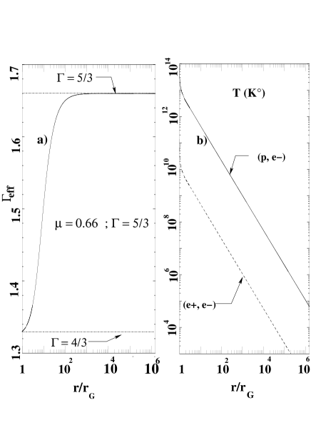
Figure 1: (a) Plot of the effective polytropic index $\Gamma_{\rm eff}$ of an adiabatic outflow showing the transition of $\Gamma_{\rm eff}$ from the ultrarelativistic value of $4/3$ to the classical one $5/3$. The corresponding temperature profile is plotted in (b) both, for electron/proton [$k_{\rm B}T=P/(2n)$] and pair plasmas [$k_{\rm B}T=P/n$] and has ultrarelativistic temperatures at the base which decrease to classical ones further out.

3 Equations in dimensionless form and parameters

3.1 Momentum and continuity equations

In the following all quantities are defined in dimensionless form. First, velocities are normalized to the speed of light $\beta=v/c$ such that $\beta_{\rm s}=v_{\rm s}/c$ is the (variable) dimensionless sound speed. Second, distances could have been normalized at the gravitational radius $r_{\rm G}$. However, we found easier to normalize all quantities at the sonic surface $r_{\star}$, such that we can define a dimensionless radius,

$$R=r/r_{\star}\,.$$ (25)

A crucial parameter of our model is

$$\mu=\frac{r_{\rm G}}{r_{\star}}=\frac{v_{\rm esc}^{2}(r_{\star})}{c^{2}}\,,$$ (26)

which is the square of the escape speed at the sonic radius normalized to the speed of light. It is also the ratio of the gravitational radius to the sonic distance. Thus $\mu$ measures the strength of the gravitational field and the distance between the central black hole and the sonic surface.

The Euler equation and the continuity equation can be written in dimensionless forms,

$$\frac{\beta^{2}-\beta_{s}^{2}}{1-\beta^{2}}\frac{{d}\ln{\beta^{2}}}{{d}R}=\frac{4\beta_{\rm s}^{2}}{R}-\frac{1-\beta_{\rm s}^{2}}{R}\frac{\mu}{R-\mu}\,.$$ (27)

$$\frac{\beta^{2}-\beta_{s}^{2}}{\beta^{2}}\frac{{d}\ln{\rho}}{{d}R}=(\Gamma-1)\left[-\frac{2}{R}+\frac{1-\beta^{2}}{\beta^{2}}\frac{1}{2R}\frac{\mu}{R-\mu}\right]\,.$$ (28)

In a nonrelativistic wind, the radius of the star is independently given from its mass. Conversely if the central object is a black hole, the gravitational radius provides a natural length scale. However, the wind cannot start and accelerate at this particular distance. In fact, it has to start at a radius $r_{o}$ located obviously above the Schwarzschild radius in the corona. In other words the wind solution should start at a dimensionless radius $R_{o}>\mu$ which will be an output of the integration starting at the sonic surface and integrating up wind.

3.2 Integration of equations and range of values of $\mu$

This model has two free parameters that affect the solution of the differential equations (27), and (28). The first parameter, $\Gamma$, is the value of the effective polytropic index at infinity. The second parameter, $\mu$, is the ratio of the Schwarzschild’s radius to the radius at the sonic surface.

Eqs. (27) and (28) have a singularity corresponding to the sonic surface, which we may call hydrodynamic horizon by analogy with the black hole horizon. At the sonic surface

the right hand sides of the two equations vanish because the left hand sides vanish.

For a detailed discussion of the nature and position of the critical surfaces in astrophysical winds, see Tsinganos et al. (1996).

This gives the following criticality condition,

$$\beta_{\rm s\star}^{2}=\frac{\mu}{4-3\mu}\,.$$ (29)

Note that the value of $\rho$ at the sonic surface, $\rho_{\star}$, follows from Eq.(18).

Since $\beta_{\rm s\star}^{2}<1$, the above criticality condition requires that we should always have $\mu<1$. Furthermore, by combining Eqs. (20) and (29) we find an upper value for $\mu$

$$\mu<\mu_{\max}=\frac{4(\Gamma-1)}{3\Gamma-1}\,.$$ (30)

Once we get the value of $\beta_{\rm s\star}$ ($\Leftrightarrow\rho_{\rm s\star}$) from the sonic criticality condition, we deduce the values of the slope of the velocity at the critical surface using De L’Hopital’s rule in Eqs. (27) and (28) which after some lengthy calculations gives

$$A{\left.\left[\frac{{d}\beta^{2}}{{d}R}\right]^{2}\right|_{\star}}+B{\left.\frac{{d}\beta^{2}}{{d}R}\right|_{\star}}+C=0$$ (31)

$$A=1+(\Gamma-1)\left.\frac{{d}\ln{\beta^{2}_{\rm s}}}{{d}\ln{\rho}}\right|_{\star}\frac{(4-3\mu)}{8(1-\mu)}\,,$$ (32)

$$B=\left.\frac{{d}\ln{\beta^{2}_{\rm s}}}{{d}\ln{\rho}}\right|_{\star}(\Gamma-1)\frac{\mu}{1-\mu}\,,$$ (33)

$$C=\frac{-16\mu^{2}}{(4-3\mu)^{3}}\left(1-\left.\frac{{d}\ln{\beta^{2}_{\rm s}}}{{d}\ln{\rho}}\right|_{\star}(\Gamma-1)\frac{(4-3\mu)^{2}}{8(1-\mu)}\right)\,.$$ (34)

As we are interested for wind type solutions, the derivative $\left.d\beta^{2}/dR\right|_{\star}$ at the sonic point should be positive. By noting that $A\,,B>0$, this is equivalent to the condition $C<0$. Then, from Eq. (34) and employing eqs. (18), (19), and (29) we get an inequality for $\mu$. We solved this numerically and found the condition $\mu>\mu_{\min}$ where the value of $\mu_{\min}$ as a function of $\Gamma$ is shown in Fig. 2 as the lower limit of the grey filled region.

Thus, the criticality conditions for wind-type solutions reduces the acceptable values of $\mu$ to a limited range:

$$\mu_{\min}<\mu<\mu_{\max}\,.$$ (35)

• $\mu_{\max}=r_{\rm G}/r_{\star,\min}$ (see Fig. 2) corresponds to the minimum distance between the Mach surface and the black hole, $r_{\star,\min}$, for which Eq. (18) has an acceptable solution $\rho_{\star}=\rho_{\star}(\beta_{\rm s\star})$. For the limiting case $r_{\star}\longrightarrow r_{\star,\min}$, $\rho_{\star}\longrightarrow\infty$. If the sonic surface is too close to the black hole, gravity becomes so important that the critical point disappears.

• $\mu_{\min}=r_{\rm G}/r_{\star,\max}$ (see Fig. 2) corresponds to the maximum distance, $r_{\star,\max}$, between the sonic surface and the black hole above which the two critical solutions are accretion-type solutions.

From Fig. 2 we see that there is a maximum value, $\Gamma=3$, beyond which $\mu_{\min}>\mu_{\max}$, because the cooling is too strong to have a wind type solution similarly to Begelman (1978).

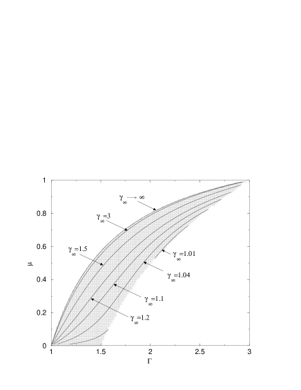
Figure 2: Contour plots of constant terminal Lorentz factor $\gamma_{\infty}$ are shown within the limiting values of $\mu$, $\mu_{\min}$ and $\mu_{\max}$ versus $\Gamma$, with the grey filled region showing the allowed wind space parameter. Note that $\mu_{\max}$ corresponds to $\gamma_{\infty}\longrightarrow\infty$.

3.3 Bernoulli constant

The conservation of the number of particle can be integrated to give a first constant of the system, which corresponds to the mass loss rate or the mass flux $\dot{m}$

$$\alpha\gamma nvr^{2}=\dot{m}\,,$$ (36)

Similarly, by integrating Euler’s equation (7), we obtain the Bernoulli equation $E=\alpha\gamma w$, which is given by

$$E=\epsilon_{0}\left(1-\frac{\mu}{R}\right)^{1/2}\frac{1}{\sqrt{1-\beta^{2}}}\frac{1+\left(1+\Gamma\right)\rho/2}{\sqrt{1+\rho}}\,.$$ (37)

Note that asymptotically ($R\rightarrow\infty$, $\rho\rightarrow 0$) the latter equation implies that the Lorentz factor is $\gamma_{\infty}=E/\epsilon_{0}$. On the other hand, by using the values of $\beta_{\star}=\beta_{\rm s\star}$ and $\rho_{\star}$ at the sonic surface

(eqs. [29] and [18]), we get the Bernoulli constant $\gamma_{\infty}=E/\epsilon_{0}$ as a function of $\Gamma$ and $\mu$, see Fig. 2.

Instead of integrating the differential equations which is the way we followed after Parker (1960), we could also plot the isocontours of constant $E$ and $\dot{m}$. The two methods are equivalent. We have checked that while integrating the differential equations $E$ remained constant.

4 Results and comparison with the nonrelativistic cases

In the following we present the results of our parametric study for various values of the polytropic index $\Gamma$ and the gravitational parameter $\mu$. We also compare them with the corresponding results in the analysis of Blumenthal & Mathews (1976) for an adiabatic polytropic index $\Gamma=5/3$ and studies using a classical equation of state with a constant polytropic index $\Gamma$.

4.1 Parametric study

We solved numerically the equations by using a Runge-Kutta scheme starting at the sonic surface

and integrating both upstream towards the black hole and downstream to infinity.

The behavior of the solutions for various values of $\mu$ is displayed in Figs. 3.

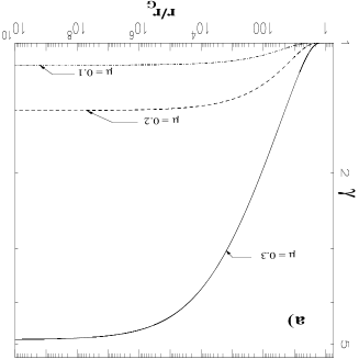
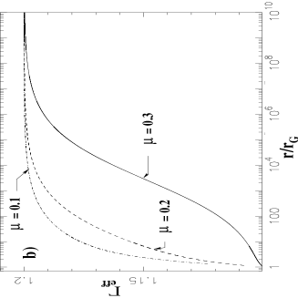
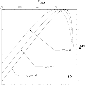
Figure 3: For $\Gamma=1.2$ we show respectively as functions of the radial distance, the Lorentz factor in (a), the effective polytropic index in (b) and the effective cross-section of the equivalent De Laval Nozzle in (c) for various wind solutions corresponding to three values of $\mu$ labeling each curve.

As $\mu$ increases the sonic surface

moves inwards closer to the compact object. Thus, the supersonic region of the outflow exposed to thermal energy deposition is enlarged. Consequently the Bernoulli energy gets larger for a given gravitational energy. This induces a better conversion of thermal energy into kinetic energy. In other words, as $\mu$ increases the distance between the corona and the black hole decreases and, to support gravity, the pressure becomes higher. The pressure driven wind passes through the critical point faster and subsequently transforms into a relativistic wind at large distances from the black hole. The situation is similar to that of nonrelativistic winds with momentum and heat addition (Leer & Holzer (1980)) wherein only for heat/momentum addition in the supersonic part of the flow the terminal wind speed increases. The mass loss is unaffected in such a case and is only affected for momentum/heat addition in the subsonic region. As illustrated by Fig. 3b, the higher is $\mu$, the more extended downstream is the area of the flow where the effective polytropic index is smaller than $\Gamma=1.2$ and thus the wind is more efficiently accelerated. This more efficient conversion of thermal energy for higher values of $\mu$ maybe also illustrated by calculating the cross-section of the equivalent De Laval Nozzle (Parker (1960)).

$$\frac{{\rm d}\ln S_{\rm eff}}{{\rm d}R}=\frac{2}{R}-\frac{1\,-\,\beta_{s}^{2}}{2\,R\,(R-\mu)}\;\frac{\mu}{\beta_{s}^{2}}$$ (38)

where $S_{\rm eff}$ is the effective cross-section. As shown in Fig. 3c, the larger is $\mu$, the larger is the opening of the effective cross-section.

4.2 Comparison with the classical wind

In the classical limit, the horizon goes to the center of the gravitational well, $r_{G}\rightarrow 0$ and consequently $\mu\rightarrow 0$. The index $\Gamma$ is the only free parameter which is left together with the mass loss rate.

Then, in the classical limit the condition at the critical point reduces to the usual expression,

$$\frac{\beta_{\rm s\star}^{2}}{\mu}=\frac{1}{4}\Leftrightarrow v_{\rm s\star}^{2}=\frac{{\cal G}{\cal M}_{\star}}{2r_{\star}}\,,$$ (39)

where the sound speed at the sonic surface

is equal to half of the escape speed. From this single relation, the distance between the stellar surface and the sonic surface is uniquely determined from the sound speed at the sonic surface

Conversely in the relativistic case $\mu$ is a free parameter, so we can change the distance between the two surfaces and increase the effect of thermal conversion in accelerating the wind.

For a classical polytropic wind there is no acceleration for $\Gamma>3/2$ (see Parker (1960)) because then the acceleration at the sonic surface

becomes negative for both critical solutions and no real wind-type solution exists. Conversely our relativistic solutions can be accelerated even if $\Gamma>3/2$ when $\mu$ increases. This is illustrated in Figs. 4a,b where the topology of the adiabatic solution ($\Gamma=5/3$) is displayed in the classical and the relativistic cases. In the first case both critical solutions are decelerated while in the second one there is an accelerated wind type solution. This is also shown in Fig. 2: for $\mu=0$ (classical limit, along the horizontal axis), the highest value of $\Gamma$ to have an accelerated wind-type solution is $1.5$. For non zero values of $\mu$ (relativistic regime), the domain of wind-type solutions extends to higher values of $\Gamma$.

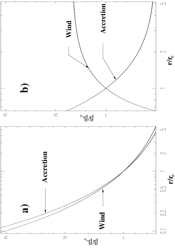
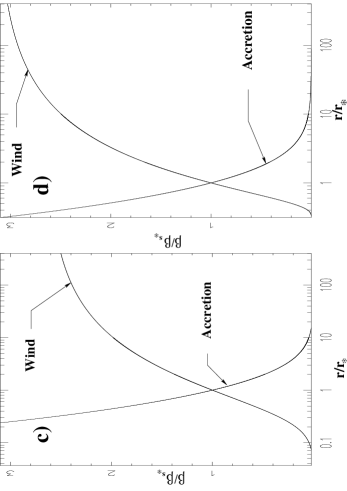
Figure 4: Comparison of the classical Parker solutions and the relativistic ones for two sets of the parameters $\Gamma$ and $\mu$. For an adiabatic polytropic index $\Gamma=5/3$ and $\mu=0.65$ in a) is shown the nonaccelerating classical Parker solutions while in b) the accelerating relativistic ones. For $\Gamma=1.2$ and $\mu=0.2$ is shown in c) the classical Parker solutions and in d) the relativistic ones.

The relativistic wind is characterized by the fact that from the compact object outwards the pressure decreases faster. This is due to the presence of the redshift function $\alpha$ in the continuity equation (36). When matter flows away from the central object the proper volume of the fluid increases faster than the observed (spherical) volume because of $\alpha$,

which provokes the decrease of the proper density and consequently of the pressure. The larger pressure gradient leads to higher acceleration. This is equivalent to the well known acceleration due to overradial flaring in the classical solar wind as studied in Kopp & Holzer (1976).

In fact, expanding Euler’s equation (27) to first order in the relativistic effects, i.e. for $\mu\ll 1$ and $\rho\ll 1$, we find

$$\frac{1}{2}\frac{(\beta/\beta_{\rm s})^{2}-1}{1-\beta^{2}}\frac{\partial\ln{\beta^{2}}}{\partial R}=$$

$$\frac{2}{R^{2}}\left(R-\frac{\beta_{\rm s\star}^{2}}{\beta_{\rm s}^{2}}\right)+\frac{3\mu}{2R^{2}}\frac{\beta_{\rm s\star}^{2}}{\beta_{\rm s}^{2}}+\frac{\Gamma\left(\Gamma-1\right)\rho}{R^{2}}\frac{\beta_{\rm s\star}^{2}}{\beta_{\rm s}^{2}}\,.$$ (40)

The first term of the right hand side is the classical term. The second term shows the effect of gravity in general relativity, related to the existence of a characteristic distance due to the metric of the black hole. This positive term increases the acceleration and the conversion of thermal energy into kinetic energy. The third term shows the influence of relativistic temperatures. It is also a positive term which increases the efficiency of the acceleration as long as the temperature remains relativistic. These two terms are responsible for the acceleration obtained even for $\Gamma>3/2$.

Even for quasi-isothermal ($\Gamma\ga 1$) flows we see that the relativistic winds are more rapidly accelerated than their classical counter part (Fig. 4c,d).

4.3 Comparison with a relativistic wind having a constant effective polytropic index

Let us consider next relativistic winds with a constant effective polytropic. In this approach the same free parameters exist, $\mu$ and $\Gamma$. However for a relativistic polytropic wind where $\Gamma_{\rm eff}=\Gamma=$const, the expression of the sound speed and the Bernoulli equation are written as

$${\beta_{\rm s_{c}}}^{2}=\Gamma\frac{(\Gamma-1)\rho_{c}}{(\Gamma-1)+\Gamma\rho_{c}}\,,\quad\rho_{c}\equiv\frac{P}{n\epsilon_{0}}\,,$$ (41)

$$E=\alpha\gamma\left(1+\frac{\Gamma}{\Gamma-1}\rho_{c}\right)\epsilon_{0}\,.$$ (42)

The main difference in the behavior of the solutions with those using the generalized equation of state appears in the zone close to the compact object where there is a transition between classical and relativistic temperatures.

For a fixed value of $\mu$, we may compare the solutions of three equations of state describing a relativistic wind. First, by using the consistent equation of state with a variable $\Gamma_{\rm eff}$ and second, for a constant polytropic index, either $\Gamma_{\rm rel}=(\Gamma+1)/2$, a value which is the limit of $\Gamma_{\rm eff}$ in the ultrarelativistic domain, or, for a constant $\Gamma_{\rm nonrel}=\Gamma$ which is the limit of $\Gamma_{\rm eff}$ in the classical regime (see Fig. 5). The consistent relativistic equation of state gives a wind which is always more efficient than the classical one corresponding to the constant value $\Gamma$, but less efficient than the ultrarelativistic one for the value $(\Gamma+1)/2$. Using the value $\Gamma$ will always underestimate the asymptotic speed, but this difference becomes smaller as we approach the adiabatic value, as illustrated in Fig. 5. Conversely, it is appropriate to use the value $(\Gamma+1)/2$ in the vicinity of the black hole where the temperatures are ultrarelativistic. However it will always overestimate the asymptotic Lorentz factor, especially in the adiabatic case.

As it can be seen in Fig. 5b, in some cases the solutions can be slightly decelerated in the super-sonic region, because the thermal energy is not sufficient to overcome gravity in these distances.

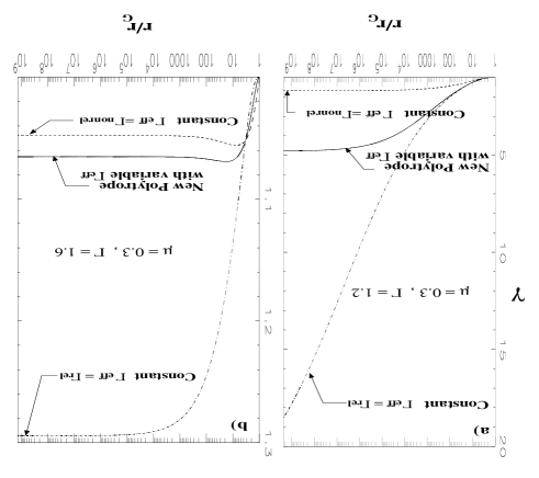
Figure 5: Comparison between a variable and two constant $\Gamma$ polytropic equations of state for two solutions with $\mu=0.3$. In the left panel $\Gamma=1.2$ while in the right panel $\Gamma=1.6$. In each panel, the two constant values $\Gamma_{\rm rel}=(\Gamma+1)/2$ and $\Gamma_{\rm nonrel}=\Gamma$ correspond to the limits of $\Gamma_{\rm eff}$ in the ultrarelativistic and the classical regimes, respectively.

In the ultrarelativistic limit (large $\mu$ and $\rho$) we can obtain analytically that our model is more efficient than the classical one, by comparing the acceleration at the sonic point for the two models. The condition is

$$\left.\frac{{d}\beta^{2}}{{d}R}\right|_{C}<\left.\frac{{d}\beta^{2}}{{d}R}\right|_{R}\,,$$ (43)

where the subscript $C$ refers to the classical polytrope, and $R$ to the relativistic one. This is fulfilled if

$$2-\frac{1-\left.\beta_{\rm s}^{2}\right|_{C}}{\left.\beta_{\rm s}^{2}\right|_{C}}\frac{1}{2}\frac{\mu}{1-\mu}>2-\frac{1-\left.\beta_{\rm s}^{2}\right|_{R}}{\left.\beta_{\rm s}^{2}\right|_{R}}\frac{1}{2}\frac{\mu}{1-\mu}\,,$$ (44)

which is equivalent to

$$\left.\beta_{\rm s}^{2}\right|_{C}<\left.\beta_{\rm s}^{2}\right|_{R}\,.$$ (45)

This condition is satisfied if the sonic surface

is close enough to the compact object. In the limit of large $\mu$, comparing Eqs. (41) and (18), we conclude that the relativistic polytrope is more efficiently accelerating the flow than the classical one if $\Gamma>1$.

At this point of the comparison, we should stress that a constant polytropic index, as it has been used in many models of relativistic thermal wind, is inconsistent with having both ultrarelativistic and classical temperatures in the flow. With the usual equation of state the thermodynamic regime is either ultrarelativistic or classical. In reality the outflow escapes from a very hot corona but cools down further out so there must be a smooth transition from one regime to the other.

5 Application

In this section we apply our model using typical values for jets from compacts objects. We consider two cases, a supermassive black hole with $M=10^{9}\,M_{\odot}$, typical of a quasar (see Wang & Zhang (2003)) and a stellar size black hole with $M=10\,M_{\odot}$, typical of a microquasar (see Mirabel (1998)).

We choose the sonic surface to be close to the compact object, $r_{\star}=6.45\,r_{\rm G}$, such that $\mu=0.155$. This choice of $\mu$ gives a sufficiently high asymptotic Lorentz factor of $\gamma\geq 5$, typical of those objects for sufficiently small values of $\Gamma$ (Fig. 6). For the solution with $\Gamma=1.09$, the initial temperature is $T\approx 10^{12}$K in the case of electron-proton gas and $T\approx\,10^{9}$K in the case of electron-positron pairs. Note however, that for low values of $\Gamma$ such as $\Gamma=1.09$ the temperature remains unrealistically high at large distances. Hence, a more physical approach would be to avoid taking these solutions corresponding to $\Gamma\ga 1$ all the way to large distances, but instead match them with solutions with a faster decrease of the temperature ($\Gamma\approx 4/3$).

In both cases the solutions differ only in the density and mass loss rate. Both solutions have the same Lorentz factor profile and the same energy per particle in units of mass energy as this depends only on $\mu$ and not on the mass of the central object or on the total mass loss rate. The result is displayed on Fig. 6.

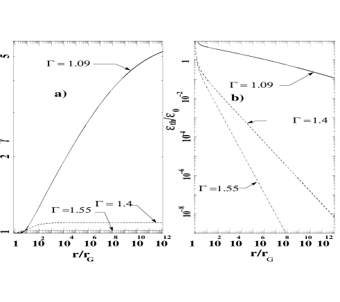
Figure 6: Plot of the Lorentz factor in (a) and the thermal energy density in (b) versus radius for $\mu=0.155$ and three different values of the polytropic parameter $\Gamma$.

For quasi-isothermal winds, $\Gamma\sim 1-1.2$, the Lorentz factor $\gamma$ can exceed a value of $5$ if the thermal energy distribution in the vicinity of the central object is roughly 10 times more than the mass energy. The thermal content is spread along the flow and not peaked close to the compact object such that it can accelerate efficiently the flow with a lower maximum in temperature. Such a quasi-isothermal outflow can occur if there is a redistribution of energy by the highly radiative initial field which cools the upstream flow and reheat the down part in the subsonic part where the medium is still optically thick (Das 2000; Tarafdar (1988)). The dissipation of disorganized magnetic field could also occur to produce extended heating. Such a dissipation has shown to be potentially important after the sonic surface and in the asymptotic region (Heinz & Begelman (2000))

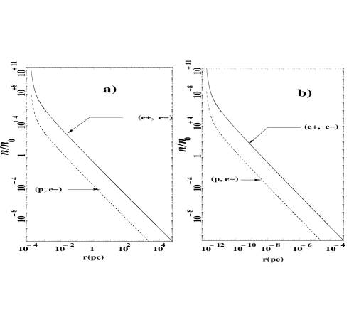
Figure 7: Plot of density versus radius for $\mu=0.155$ and $\Gamma=1.09$ for the quasar solution in (a) and the microquasar solution in (b).

In Fig. 7 we plot the number density in units of $n_{0}$ cm^-3 as a function of distance, for a free density parameter $n_{0}$. For the quasar solution (Fig. 7a) the corresponding mass loss rate is $\dot{M}_{\rm quasar}=10^{-6}n_{0}\,\dot{M}_{\rm Eddington}=1.41\times 10^{-6}n_{0}\,M_{\odot}/$yr, while for the micro-quasar solution (Fig. 7b) $\dot{M}_{\mu\rm quasar}=10^{-14}n_{0}\,\dot{M}_{\rm Eddington}=1.41\times 10^{-22}n_{0}\,M_{\odot}/$yr.

We note that as the mass of the central compact object changes from $10^{9}M_{\odot}$ to $10M_{\odot}$ the solution is simply scaled down spatially, a result consistent with the idea that microquasars could be considered to zeroth order as

scaled down versions of quasars. A more detailed treatment however, should take into account certain differences of the two cases, e.g. pair production, different densities, etc., something beyond the scope of the present analysis.

6 Conclusion

We have generalized a variable polytropic index equation of state for the purpose of modelling relativistic flows, both in temperature and velocity in the vicinity of a Schwarzschild black hole. This has enabled us to analyze thermally driven winds having both ultrarelativistic temperatures at the base of the central corona ($k_{\rm B}T\ga\epsilon_{0}$) and classical temperatures ($k_{\rm B}T\ll\epsilon_{0}$) further out. This equation of state is characterized by a polytropic index $\Gamma$ such that pressure is related to density in the form of Eq. (15).

For a given polytropic index $\Gamma$, transonic wind solutions can be found only within a limited range of radii of the sonic point, $r_{*}$,

$$\frac{1}{\mu_{\max}}<\frac{r_{\star}}{r_{\rm G}}<\frac{1}{\mu_{\min}}\,.$$

This sonic transition should be far enough from the Schwarzschild radius $r_{\rm G}$ such that gravity is not too high to allow the existence of critical solutions, because for too strong gravity the flow cannot escape, even if the temperature is infinite. On the other hand, the sonic transition should also be close enough such that the corona is not too diluted and the pressure too low to obtain an accelerated transonic solution.

Schwarzschild’s metric tends to enhance the effects of gravity. One major effect of strong gravity is to have a more efficient De Laval nozzle which allows to have accelerated winds even for polytropic indices larger than the typical Parker’s value, i.e. $\Gamma>3/2$, conversely to the classical Parker’s wind (Parker (1960)). This can be understood by computing the effective polytropic index ${d}\ln P/{d}\ln\rho$. Enhanced gravity and also relativistic temperatures tend to lower the effective polytropic index in the low corona which gives a more efficient thermal driving of the wind.

However, we note that despite its widespread use in the literature, the ordinary polytropic equation of state with a constant effective polytropic index seems not to be really consistent with a mixed regime of temperatures in the corona from ultra-relativistic to classical ones.

In order to reach very high Lorentz factors, in the adiabatic case, the internal energy of the plasma in the corona should exceed by a large factor its mass energy. This can be easily achieved if the total pressure is not limited to the kinetic pressure of the gas but also includes extra physical processes such as MHD waves or radiation. This result is somehow consistent with the usual low velocities obtained for classical winds. Quasi-isothermal winds reach higher Lorentz factors with a relatively lower – but still larger than the mass energy – internal energy.

Applying our model to typical values observed in microquasars and quasars we recover as expected that microquasar outflows may be seen as a scaled down version of their bigger extragalactic counterparts. We do not claim however that all jets are only thermally driven. A magnetic driving mechanism seems more efficient indeed to accelerate the outflow on parsec scales as shown by Vlahakis & Königl (2004), in agreement with some jet observations (Sudou et al. (2000)). However, we simply emphasize that thermal driving may indeed play an important role alongside other mechanisms, when hot coronae are observed; in such cases, a consistent way of dealing with these relativistic temperatures is required.

Finally, this consistent generalization of the Parker polytrope for relativistic thermal winds could be implemented in numerical simulations, instead of the classical constant polytropic index equation of state to simulate the transition from relativistic to nonrelativistic temperatures along the flow. Nevertheless, as in any polytropic equation of state the source of heating is not specified on physical grounds and more detailed physics of the coronal heating is needed.

Appendix A Heating of polytropic flows

Conversely to the usual polytropic equation of state used in studying stellar interiors, the use in classical as well as relativistic winds of a polytropic index different from the adiabatic one is an implicit way to mask extra heating in the corona as explained in Sauty et al. (1999). In all cases, the fluid remains a monoatomic plasma of electrons and protons with a ratio of specific heats $5/3$.

Thus, by substituting Eq. (14) to Eq. (13), we have introduced implicitly that the external medium could give extra energy to the fluid. $e$ in Eq. (14) is the total internal energy of the gas. It has two component, i.e. $e_{\rm plasma}$ the internal energy of the plasma itself calculated from Eq. (13)

$$e_{\rm plasma}^{2}=\epsilon_{0}^{2}+\kappa n^{\frac{2}{3}}=\epsilon_{0}^{2}+\kappa n^{\Gamma_{\rm ad}-1}\,,$$ (46)

and the heating integrated along the streamline from the source $Q$. From a different point of view $Q$ is also the internal energy (defined within an arbitrary constant of course) of the external medium (also called in thermodynamics “universe” as opposed to the system) which is given to the system through heating.

The global system plasma $+$ external medium being isolated, it is adiabatic, so it is usual to define $e$ instead of $e_{\rm plasma}$ in order to keep its simple form to the energy conservation given by Eq. (2) (e.g., Blumenthal & Mathews (1976); Mobarry & Lovelace (1986)). It is easy to calculate the heating transfered to the plasma during its expansion,

$$Q=e-e_{\rm plasma}\,,$$ (47)

which is in our case given by

$$Q=\sqrt{\epsilon_{0}^{2}+\kappa n^{\Gamma-1}}-\sqrt{\epsilon_{0}^{2}+\kappa n^{(5/3)-1}}\,.$$ (48)

The same holds for the enthalpy. $w$ is the total enthalpy of the gas and the external medium and if $w_{\rm plasma}$ is the real enthalpy of the gas itself,

$$w=w_{\rm plasma}+Q\,.$$ (49)

References

- Begelman (1978) Begelman, M. C. 1978, A&A, 70, 538
- Blumenthal & Mathews (1976) Blumenthal, G. R., & Mathews, W. G. 1976, ApJ, 203, 714
- Biretta et al. (1999) Biretta, J. A., Sparks, W. B., & Macchetto, F. 1999, ApJ, 520, 621
- Bondi (1952) Bondi, H. 1952, MNRAS, 112, 195
- Chakrabarti et al. (1996) Chakrabarti, S. K., Titarchuk, L., Kazanus, L., & Ebisawa, K. 1996, A&AS, 120, 163
- Chattopadhyay et al. (2004) Chattopadhyay, I., Das, S., & Chakrabarti, S. K. 2004, MNRAS, 348, 846
- Corbel et al. (2003) Corbel, S., Nowak, M. A., Fender, R. P., Tzioumis, A. K., & Markoff, S. 2003, A&A, 400, 1007
- Daigne & Drenkhahn (2002) Daigne, F., & Drenkhahn, G. 2002, A&A, 381, 1066
- Das (1999) Das, T. K. 1999, MNRAS, 308, 201
- Das (2000) Das, T. K. 2000, MNRAS, 318, 294
- Ferrari et al. (1985) Ferrari, A., Trussoni, E., Rosner, R., & Tsinganos, K. 1985, ApJ, 294, 397
- Heinz & Begelman (2000) Heinz, S., & Begelman, M. C. 2000, ApJ, 535, 104
- Kopp & Holzer (1976) Kopp, R. A., & Holzer, T. E. 1976, Sol. Phys., 49, 43
- Leer & Holzer (1980) Leer, E., & Holzer, T. E. 1980, J. Geophys. Res., 85, 4681
- Livio (2002) Livio, M. 2002, Nature, 417, 125L
- Mathews (1971) Mathews, W. G. 1971, ApJ, 165, 147
- Michel (1972) Michel, F. C. 1972, Ap&SS, 15, 153
- Mirabel (1998) Mirabel, I. F., & Rodriquez, L. F. 1998, Nature, 392, 673
- Mobarry & Lovelace (1986) Mobarry, C. M., & Lovelace, R. V. E. 1986, ApJ, 309, 455
- Parker (1960) Parker, E. N. 1960, ApJ, 137, 821
- Rózańska & Czerny (2000) Rózańska, A., & Czerny, B. 2000, A&A, 360, 1170
- Sauty et al. (1999) Sauty, C., Tsinganos, K., & Trussoni, E. 1999, A&A, 348, 327
- Synge (1957) Synge, J. L., 1957, The Relativistic Gas (New York: InterScience)
- Sudou et al. (2000) Sudou, et al. 2000, PASJ, 52, 989
- Tarafdar (1988) Tarafdar, S. F. 1988, ApJ, 331, 932
- Tsinganos et al. (1996) Tsinganos, K., Sauty, C., Surlantzis, G., Trussoni, E., Contopoulos, J. 1996, MNRAS, 283, 111
- Vlahakis & Königl (2004) Vlahakis, N., & Königl, A., 2004, ApJ, 605, 656
- Wang & Zhang (2003) Wang, T.-G., & Zhang, X.-G. 2003, MNRAS, 340, 793