Warm water vapor envelope in Mira variables and its effects on the apparent size from the near-infrared to the mid-infrared

We present a possible interpretation for the increase of the angular diameter of the Mira variables $o$ Cet, R Leo, and $\chi$ Cyg from the $K$ band to the 11 $\mu$m  region revealed by the recent interferometric observations using narrow bandpasses where no salient spectral feature is present (Weiner et al. 2003a , 2003b ). A simple two-layer model consisting of hot and cool H₂O layers for the warm water vapor envelope, whose presence in Mira variables was revealed by previous spectroscopic observations, can reproduce the angular diameters observed with Infrared Spatial Interferometer as well as the high-resolution TEXES spectra obtained in the 11 $\mu$m region. The warm water vapor layers are optically thick in the lines, and therefore, strong absorption due to H₂O can be expected from such a dense water vapor envelope. However, the absorption lines are filled in by emission from the extended part of the envelope, and this results in the high-resolution 11 $\mu$m  spectra which exhibit only weak, fine spectral features, masking the spectroscopic evidences of the dense, warm water vapor envelope. On the other hand, the presence of the warm water vapor envelope manifests itself as the larger angular diameters in the 11 $\mu$m  region as compared to those measured in the near-infrared. Furthermore, comparison of the visibilities predicted in the near-infrared (1.5–3.8 $\mu$m) with observational results available in the literature demonstrates that our two-layer model for the warm water vapor envelope can also reproduce the observed near-infrared visibilities and angular diameters, and suggests that the wavelength dependence of the angular size of Mira variables in the infrared largely reflects the H₂O opacity. The radii of the hot H₂O layers in the three Mira variables are derived to be 1.5–1.7 $R_{\star}$  with temperatures of 1800–2000 K and H₂O  column densities of $(1\mbox{--}5)\times 10^{21}$ cm^-2, while the radii of the cool H₂O layers are derived to be 2.2–2.5 $R_{\star}$ with temperatures of 1200–1400 K and H₂O  column densities of $(1\mbox{--}7)\times 10^{21}$ cm^-2.

1 Introduction

An increase of the angular size from the near-infrared toward longer wavelengths appears to be a common phenomenon observed in various classes of cool luminous stars such as M (super)giants and Mira variables. Mennesson et al. (mennesson02 (2002)) revealed that the uniform disk (UD) diameters of semiregular M giants as well as Mira variables measured in the $L^{\prime}$ band are 20–100% larger than those measured in the $K^{\prime}$ band. Recently, Weiner et al. (weiner00 (2000), 2003a , and 2003b , hereafter W00, WHT03a, and WHT03b, respectively) have measured the angular size at 11 $\mu$m for the M supergiants $\alpha$ Ori and $\alpha$ Her as well as the Mira variables $o$ Cet, R Leo, and $\chi$ Cyg, using the Infrared Spatial Interferometer (ISI) with a spectral bandwidth of 0.17 cm^-1. They found that the uniform disk diameters of the two M supergiants measured at 11 $\mu$m are $\sim$30% larger than those measured in the $K$ band, while the 11 $\mu$m uniform disk diameters of the three Mira variables are roughly twice as large as those measured in the $K$ band.

Although these Mira variables exhibit dust emission from the circumstellar envelope, the observed increase of the angular diameter from the near-infrared to the mid-infrared cannot simply be attributed to the dust shell, as discussed in detail by WHT03a. The radii of the inner boundary of the circumstellar dust shell are estimated to be 2–4 $R_{\star}$ for $o$ Cet and R Leo, and $\sim$20 $R_{\star}$ for $\chi$ Cyg (Danchi et al. danchi94 (1994), Schuller et al. schuller04 (2004)), and such extended dust shells are completely resolved with the baselines of 20–56 m used in the ISI observations by W00, WHT03a, and WHT03b. In other words, the visibility component resulting from the dust shell is nearly zero at these baseline lengths, and the effect of the dust shell is to lower the total visibility by an amount equal to the fraction of flux originating in the dust shell in the field of view. This effect is already taken into account in the determination of the uniform disk diameters by W00, WHT03a, and WHT03b, and therefore, it is unlikely that the extended dust shell causes the 11 $\mu$m angular size to appear larger than in the near-infrared.

Instead, the increase of the angular size from the $K$ band to the $L^{\prime}$ band as well as to the 11 $\mu$m region can be attributed to extended gaseous layers close to the photosphere. Mennesson et al. (mennesson02 (2002)) conclude that the observed increase of the angular diameter from the $K^{\prime}$ band to the $L^{\prime}$ band can be explained by an optically thin layer ($\tau\approx 0.5$) extending to $\sim$3 $R_{\star}$ with a (pseudo)continuous opacity. Perrin et al. (perrin04 (2004)) apply a similar model to interferometric observations of $\alpha$ Ori and $\alpha$ Her obtained in the $K$ and $L$ bands as well as in the 11 $\mu$m region, and conclude that the extended gaseous layer is optically thin in the $K$ and $L$ bands ($\tau_{K}=0.06$ and $\tau_{L}=0.026$), but optically thick in the 11 $\mu$m region ($\tau_{11\mu{\rm m}}=2.33$). Both Mennesson et al. (mennesson02 (2002)) and Perrin et al. (perrin04 (2004)) suspect opacities due to molecular species such as H₂O, CO, and SiO as the source of the (pseudo)continuous opacity. The presence of such a warm molecular envelope is already confirmed by analyses of infrared molecular spectra. Tsuji (tsuji78 (1978)) interpreted infrared spectral data of the M supergiant $\mu$ Cep and the Mira variable R Cas in terms of a warm water vapor envelope, and Tsuji (tsuji88 (1988)) further found evidence of the presence of the warm molecular envelope in the high-resolution spectra of M (super)giants. More recently, infrared spectra obtained with the Short Wavelength Spectrometer (SWS) onboard the Infrared Space Observatory (ISO) have provided ample information on physical parameters of the warm molecular envelope (e.g., Tsuji et al. tsuji97 (1997), Yamamura et al. yamamura99 (1999), Cami et al. cami00 (2000), Matsuura et al. matsuura02 (2002)).

However, the high-resolution 11 $\mu$m spectra of the M supergiants $\alpha$ Ori and $\alpha$ Her as well as the Mira variables $o$ Cet, R Leo, and $\chi$ Cyg presented by WHT03a and WHT03b turn out to pose difficulty in interpreting the increase of the angular diameter in terms of the extended, warm water vapor envelope. These 11 $\mu$m spectra were obtained using the TEXES instrument mounted on the Infrared Telescope Facility telescope with a spectral resolution of $\sim$10⁵ (Lacy et al. lacy02 (2002)). The high-resolution TEXES spectra of the above M supergiants and Mira variables reveal that no salient spectral features are present within the bandpasses used in the ISI observations, and therefore, these spectroscopic observations appear to be in contradiction with the interpretation that the dense, warm water vapor envelope is responsible for the increase of the angular size from the near-infrared to the 11 $\mu$m region.

Ohnaka (ohnaka04 (2004), hereafter Paper I) demonstrates that the warm water vapor envelope extending to 1.4–1.5 $R_{\star}$ with temperatures of $\sim$2000 K and H₂O column densities of the order of $10^{20}$ cm^-2 can reproduce the observed increase of the angular diameter from the near-infrared to the 11 $\mu$m region in $\alpha$ Ori and $\alpha$ Her and, simultaneously, their featureless high-resolution spectra at 11 $\mu$m. While significant absorption is expected from such a warm water vapor envelope, the absorption lines are filled in by the emission of H₂O lines from the extended part of the envelope, which leads to spectra without any conspicuous spectral features as observed with the TEXES instrument. On the other hand, the emission from the extended water vapor envelope causes the apparent size of the objects to be significantly larger than the photospheric size, in agreement with the interferometric observations with ISI presented by WHT03b.

If the warm water vapor envelope is present even in early M supergiants such as $\alpha$ Ori and $\mu$ Cep and causes the stellar angular size in the mid-infrared to appear larger than that measured in the near-infrared, it can also be the case for Mira variables, for which water vapor is known to be present in the photosphere and we can expect even denser water vapor envelopes than in early M supergiants. In the present paper, we attempt to interpret the increase of the angular diameter from the near-infrared to the 11 $\mu$m region as well as the high-resolution 11 $\mu$m TEXES spectra observed for the Mira variables $o$ Cet, R Leo, and $\chi$ Cyg in terms of the warm water vapor envelope.

2 Modeling of the warm water vapor envelope

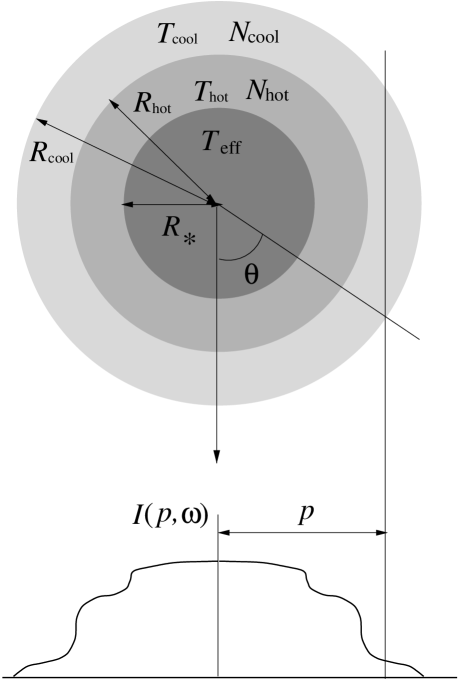
Figure 1: The model used in the present work. The photosphere is approximated by a blackbody of $T_{\rm eff}$ with a radius $R_{\star}$. The column densities in the radial direction ($N_{\rm hot}$ and $N_{\rm cool}$) and the temperatures of H₂O gas ($T_{\rm hot}$ and $T_{\rm cool}$) as well as the radii of the water vapor layers ($R_{\rm hot}$ and $R_{\rm cool}$) are the input parameters.

In our model, the central star is surrounded by a warm water vapor envelope, which consists of two layers with different temperatures $T_{\rm hot}$ and $T_{\rm cool}$, as depicted in Fig. 1. The central star is approximated by a blackbody of effective temperature $T_{\rm eff}$ with a radius $R_{\star}$. The temperature and the density are assumed to be constant in these hot and cool layers, which extend to $R_{\rm hot}$ and $R_{\rm cool}$, respectively. We denote the column density of H₂O in the radial direction in the hot and cool layers as $N_{\rm hot}$ and $N_{\rm cool}$, respectively. As very simple it may seem, such a two-layer model turned out to be successful in interpreting infrared molecular spectra obtained with ISO/SWS. For example, Yamamura et al. (yamamura99 (1999)) and Matsuura et al. (matsuura02 (2002)) could reproduce H₂O spectra of Mira variables obtained with ISO/SWS using a two-layer model, although their two-layer model consists of a stack of plane-parallel slabs, instead of spherical layers as adopted in the present work.

We adopt an effective temperature of 3000 K for the Mira variables studied in the present work. While the effective temperatures of Mira variables are known to show temporal variations with phase (e.g., van Belle et al. vanbelle96 (1996), Perrin et al. perrin99 (1999), Woodruff et al. woodruff04 (2004)), the effect of the uncertainty of the effective temperature adopted in our model turns out to be minor as we show below, because the warm water vapor envelope is quite optically thick in the wavelength regions discussed in the present work.

We first calculate the line opacity due to H₂O assuming a Gaussian profile. We adopt a velocity of 5 km s^-1 for the sum of the thermal velocity and the micro-turbulent velocity. The $g\!f$-values and the lower excitation potentials of H₂O lines are calculated using the HITEMP line list (Rothman rothman97 (1997)) and the list compiled by Partridge & Schwenke (partridge97 (1997), hereafter PS97). The HITEMP line list is an extension of the HITRAN database toward high temperatures expected in stellar atmospheres, and the HITEMP H₂O line list used here is calculated for a temperature of 1000 K. As we demonstrate below, the temperature of the warm water vapor envelope can be as high as $\sim$2000 K, and therefore, the HITEMP H₂O line list for 1000 K may not be adequate for such a high temperature. The PS97 H₂O line list is generated for a temperature of 4000 K and appears to be the most extensive line list of H₂O up to date. We use both line lists for our calculation to study possible effects of the difference between the two H₂O line lists.

The energy level populations of H₂O are calculated assuming local thermodynamical equilibrium (LTE). We examine the validity of LTE in the temperature and density ranges relevant for the present work, using the order-of-magnitude estimates of collisional and radiative de-excitation rates, as adopted in Paper I. The collisional de-excitation rate $C_{\rm ul}$ is given by $C_{\rm ul}\sim\!N\sigma_{\rm ul}v_{\rm rel}$, where $N$ is the density of the primary collision partner, $\sigma_{\rm ul}$ is the cross section, which we approximate with the geometrical cross section, and $v_{\rm rel}$ is the relative velocity between the collision partner species and H₂O molecules. As we will show below, for the hot layer of the warm water vapor envelope in $o$ Cet, R Leo, and $\chi$ Cyg, the column density of H₂O is found to be of the order of $10^{21}$ cm^-2 with temperatures of 1800–2000 K, and the geometrical thickness is derived to be $\sim$0.5 $R_{\star}$, which translates into $1\times 10^{13}$ cm with a stellar radius of 300 $R_{\sun}$ assumed. The number density of H₂O is then estimated to be $1\times 10^{8}$ cm^-3. For temperatures and densities found in the hot layer of the warm water vapor envelope, H atoms appear to be the primary collision partner of H₂O molecules, and the ratio of the number density of H atoms to that of H₂O molecules expected in chemical equilibrium is approximately $10^{4}$ for the relevant temperatures and densities. Therefore, the number density of H atoms in the hot layer is estimated to be $\sim\!1\times 10^{12}$ cm^-3. With a geometrical cross section $\sigma_{\rm ul}$ of $10^{-15}$ cm² and a relative velocity $v_{\rm rel}$ of 5 km s^-1 assumed, this number density of H atoms leads to a collisional de-excitation rate of $\sim\!500$ s^-1. For the cool component of the water vapor envelope, we derive temperatures of 1200–1400 K, geometrical thicknesses of $\sim\!1.5$ $R_{\star}$, and H₂O column densities of the order of $10^{21}$ cm^-2, which leads to a number density of H₂O of $\sim\!3\times 10^{7}$ cm^-3. At these temperatures and densities, H₂ molecules are the main collision partner of H₂O molecules, and the ratio of the number density of H₂ molecules to that of H₂O molecules expected in chemical equilibrium is $\sim\!3\times 10^{3}$, which leads to a collisional de-excitation rate of $\sim\!50$ s^-1. On the other hand, the rate of spontaneous emission can be estimated from the Einstein coefficients $A_{\rm ul}$. For the H₂O molecule, the ranges of $A_{\rm ul}$ are approximately $\sim\!\!10^{-4}$–$3\times 10^{2}$ s^-1, $\sim\!\!10^{-5}$–$3\times 10^{2}$ s^-1, and $\la 10$ s^-1 in the 11 $\mu$m region, $K$ band, and $L^{\prime}$ band, respectively. Therefore, for these wavelength regions we will discuss below, the assumption of LTE is valid for weak and moderately strong H₂O lines both in the hot and cool layers of the warm water vapor envelope, while non-LTE effects may not be negligible for very strong lines. However, a comprehensive calculation with non-LTE effects taken into account is beyond the scope of the present paper, and we assume LTE for the H₂O lines considered here.

Once the line opacity has been obtained, the monochromatic intensity profile as well as the spectrum (emergent flux) can be calculated at an appropriate wavenumber interval, as described in Paper I. In order to compare with the observed TEXES spectra of the three Mira variables, synthetic spectra are spectrally convolved with a Gaussian profile which represents the effects of the spectral resolution of the instrument as well as of the macro-turbulent velocity in the atmosphere of the Mira variables. The spectral resolution of the TEXES instrument is $10^{5}$, which translates into an instrumental broadening of 3 km s^-1. The macro-turbulent velocity in the atmosphere of Mira variables is not well known. For non-Mira M giants, however, analyses of high-resolution spectra are available, and they may be used as a guide to estimate the macro-turbulent velocity in the atmosphere of Mira variables. Tsuji (tsuji86 (1986)) analyzed the CO first-overtone bands of non-Mira K and M giants and obtained macro-turbulent velocities ranging from $\sim$1 km s^-1 to $\sim$4 km s^-1. In the present work, we tentatively assume a macro-turbulent velocity of 3 km s^-1 for the three Miras, and the FWHM of the Gaussian profile to represent the spectral resolution of the instrument and the macro-turbulent velocity is calculated as $\sqrt{3^{2}+3^{2}}=4.24$ km s^-1. The spectrum convolved with this Gaussian profile and normalized, $F_{\omega}$, is then diluted as follows, taking the effect of continuous dust emission from the circumstellar dust shell into account:

$$F_{\omega}^{\rm diluted}=(1-f_{\rm dust})F_{\omega}+f_{\rm dust}\,,$$ (1)

where $F_{\omega}^{\rm diluted}$ is the final spectrum and $f_{\rm dust}$ is the fraction of the flux contribution of the circumstellar dust shell.

We calculate the monochromatic visibility from the monochromatic intensity profile at each wavenumber using the Hankel transform, and then the monochromatic visibility is spectrally convolved with an appropriate response function which represents the spectral resolution of the interferometric observation at issue. For the ISI observations we will discuss below, WHT03a and WHT03b used narrow bandpasses with a width of 0.17 cm^-1. Therefore, the spectral response function is assumed to be a top-hat function with a width of 0.17 cm^-1.

We compare synthetic spectra and uniform disk diameters with the TEXES spectra as well as the 11 $\mu$m uniform disk diameters obtained by WHT03a and WHT03b, searching for a parameter set which can best reproduce these observational results. The ranges of the input parameters are as follows: $T_{\rm hot}$ (K) = 1600 … 2000 with $\Delta\mbox{$T_{\rm hot}$}=100$ K, $T_{\rm cool}$ (K) = 1000 … 1400 with $\Delta\mbox{$T_{\rm cool}$}=100$ K, $R_{\rm hot}$ ($R_{\star}$) = 1.3, 1.5, 1.7, and 2.0, and $R_{\rm cool}$ ($R_{\star}$) = 2.0, 2.2, 2.5, 2.7, and 3.0 with a condition $\mbox{$R_{\rm hot}$}<\mbox{$R_{\rm cool}$}$. The grid for $N_{\rm hot}$ (cm^-2 ) and $N_{\rm cool}$ (cm^-2 ) is $10^{19}$, $10^{20}$, $5\times 10^{20}$, $10^{21}$, $3\times 10^{21}$, $5\times 10^{21}$, $7\times 10^{21}$, and $10^{22}$. The uncertainties of the derived temperatures and radii of the H₂O layers are estimated to be $\pm 100$ K and $\pm 0.2$ $R_{\star}$, respectively, while the uncertainties of the H₂O column densities are approximately a factor of 2. The adoption of an effective temperature of 2800 K, instead of 3000 K, leads to no noticeable changes in the spectra and visibilities discussed in the present work. In the next section, we discuss comparison between observation and model for each object.

3 Comparison with the observed spectra and angular diameters

3.1 $o$ Cet

3.1.1 11 $\mu$m spectrum

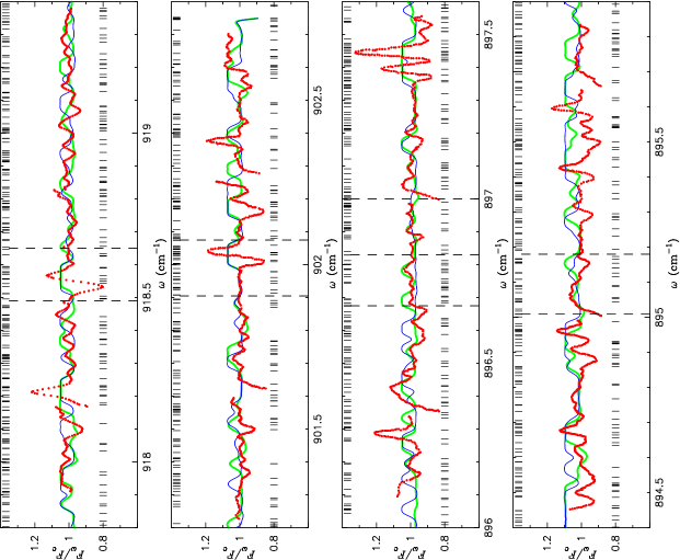
Figure 2: Spectra of $o$ Cet in the 11 $\mu$m region at phase 0.36. The red dots represent the observed spectrum of $o$ Cet presented in WHT03a, while the green and blue solid lines represent the calculated spectra using the HITEMP database and the PS97 line list, respectively. The parameters of the best-fit model for $o$ Cet are $T_{\rm hot}$ = 1800 K, $R_{\rm hot}$ = 1.5 $R_{\star}$, $N_{\rm hot}$ = $5\times 10^{21}$ cm^-2, $T_{\rm cool}$ = 1400 K, $R_{\rm cool}$ = 2.2 $R_{\star}$, and $N_{\rm cool}$ = $1\times 10^{21}$ cm^-2. The synthetic spectra are convolved with a Gaussian with a FWHM of 0.013 cm^-1 to account for the effects of the instrument as well as of the macro-turbulent velocity, and are redshifted by 83 km s^-1 to match the observation. The dashed lines represent the bandpasses used in the ISI observations. The positions of the H₂O lines whose intensity at 2000 K is stronger than $1\times 10^{-24}$ cm molecule^-1 are marked with upper ticks (PS97 line list) and lower ticks (HITEMP database). These line positions are also redshifted by 83 km s^-1 with respect to the rest wavenumber.

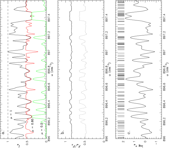
Figure 3: a: 11 $\mu$m spectra predicted from the best-fit model for $o$ Cet at the stellar disk center ($\mu=1$, top spectrum), near the limb of the warm H₂O envelope ($\mu=0.2$, bottom spectrum), and between the disk center and the limb ($\mu=0.85$, middle spectrum). The continuum level is shown with the dashed line, and the HITEMP database is used in the calculation. The flux contribution of dust emission is not included in the spectra shown. b: The dotted line represents the spectrum (emergent flux) expected for the whole object (stellar disk + warm water vapor envelope) without the dilution effect due to dust emission. The solid line represents the final spectrum with a flux contribution of dust emission of 70% taken into account. c: Optical depth in the radial direction due to H₂O lines in the same spectral region. The positions of the H₂O lines are marked with ticks. The spectra and the flux shown in a and b as well as the optical depth shown in c are redshifted by 83 km s^-1 with respect to the rest wavenumber to match the observed spectrum shown in Fig. 2, but not convolved with the Gaussian representing the instrumental effect and the macro-turbulent velocity.

For $o$ Cet, we find that the 11 $\mu$m spectrum observed at phase 0.36, which is presented in WHT03a, as well as the 11 $\mu$m uniform disk diameters obtained by W00 and WHT03a can be best reproduced by a model with $T_{\rm hot}$ = 1800 K, $R_{\rm hot}$ = 1.5 $R_{\star}$, $N_{\rm hot}$ = $5\times 10^{21}$ cm^-2, $T_{\rm cool}$ = 1400 K, $R_{\rm cool}$ = 2.2 $R_{\star}$, and $N_{\rm cool}$ = $1\times 10^{21}$ cm^-2. Figure 2 shows the synthetic spectra in the 11 $\mu$m region predicted by the best-fit model for $o$ Cet, together with the TEXES spectrum obtained at phase 0.36, which was read off Fig. 2 in WHT03a. The synthetic spectrum calculated with the HITEMP H₂O line list is represented by the green solid line, while that calculated with the PS97 H₂O line list is represented by the blue solid line. The synthetic spectra are redshifted by 83 km s^-1 to match the observation (see WHT03a). WHT03a derived the fraction of the flux contribution of the stellar disk of $o$ Cet ranging from 0.24 to 0.47 at 11 $\mu$m, which corresponds to the fraction of the flux contribution of the dust shell between 0.76 and 0.53. We adopted $f_{\rm dust}=0.7$ in our calculation of the 11 $\mu$m region for $o$ Cet. While the synthetic spectrum calculated with the PS97 line list shows H₂O features which are not seen in the spectrum calculated with the HITEMP database, the discrepancy between the two synthetic spectra is not very serious or systematic for the temperatures and densities relevant for the present calculation, given the uncertainties of the line positions of both line lists. For example, Ryde et al. (ryde02 (2002)) found that the uncertainty of the positions of H₂O pure rotation lines around 12 $\mu$m predicted by PS97 is $\sim$0.05 cm^-1. On the other hand, the uncertainty of H₂O line positions in the HITEMP database is between $\sim$0.1 and $\sim$1.0 cm^-1. Figure 2 shows that the two synthetic spectra can reproduce the approximate depths and heights of the observed fine spectral features and, in particular, the observed spectra free from any conspicuous spectral features in the bandpasses at around $\sim$896.83 cm^-1 and $\sim$895.1 cm^-1 (dashed lines) used for the ISI observations. In these bandpasses, a number of H₂O lines are present, as marked by the ticks in Fig. 2. The continuum-like appearance of the spectra is a result of the filling-in of the absorption lines by emission from the extended part of the warm water vapor envelope, as we will discuss below. On the other hand, the match for the individual line profiles is not very good, which can partially be attributed to the uncertainties of the line positions predicted by both line lists, but it is also due to the simplicity of our model, which cannot account for complicated physical and chemical processes taking place in the outer atmosphere of Mira variables. For example, the strong H₂O lines at 897.40, 897.45, 902.04, and 918.57 cm^-1 show inverse P-Cygni profiles, which suggest an inflow with a velocity of 11 km s^-1. Such a dynamical process is not taken into account in our model, and therefore, these line profiles cannot be well reproduced by our two-layer model.

The continuum-like appearance of the spectrum of $o$ Cet in the 11 $\mu$m region can be explained by the filling-in effect due to H₂O line emission from the extended part of the warm water vapor envelope. This effect is illustrated in Fig. 3, where the spectra expected at the disk center ($\mu=1$, where $\mu\equiv\cos\theta$ with $\theta$ defined in Fig. 1), at a position between the disk center and the limb ($\mu=0.85$), and near the limb ($\mu=0.2$) are shown in the top panel. The bottom panel of Fig. 3 shows the optical depth of the water vapor envelope, and the figure reveals that the water vapor envelope is optically thick ($\tau_{\omega}\approx 1$–60). These spectra as well as the optical depth are calculated with the HITEMP database. The H₂O lines appear as strong absorption in the spectrum at the disk center, as the top spectrum in Fig. 3a shows. On the other hand, the spectrum near the limb (bottom spectrum in Fig. 3a) shows emission at the positions of the H₂O lines, and these emission lines originate in the cooler H₂O layer. The spectrum for a line of sight between the disk center and the limb (middle spectrum in Fig. 3a) is dominated by the H₂O emission lines originating in the hotter layer overlaid by the H₂O absorption lines originating in the cooler layer. Since the spectrum (emergent flux) of the object is obtained by integrating the intensity over the area that the object projects onto the plane of the sky, the absorption due to H₂O lines is significantly filled in by emission from the limb, resulting in the spectrum showing only moderately strong emission features, as plotted with the dotted line in Fig. 3b. These emission features are further weakened by dilution due to continuous dust emission, as the final spectrum (solid line) in Fig. 3b shows.

The parameters derived above are similar to those derived by Yamamura et al. (yamamura99 (1999)) for $o$ Cet at phase 0.99: $T_{\rm hot}$ = 2000 K, $R_{\rm hot}$ = 2.0 $R_{\star}$, $N_{\rm hot}$ = $3.0\times 10^{21}$ cm^-2, $T_{\rm cool}$ = 1400 K, $R_{\rm cool}$ = 2.3 $R_{\star}$, and $N_{\rm cool}$ = $3.0\times 10^{20}$ cm^-2. However, it is not straightforward to discuss the phase dependence of these physical properties, not only because of the uncertainties of the derived parameters, but also because of the phase dependence of the stellar continuum radius. The analysis by Woodruff et al. (woodruff04 (2004)) demonstrates that the stellar radius of $o$ Cet in the 1.04 $\mu$m  continuum predicted by dynamical model atmospheres shows a sinusoidal variation from phase 0.0 to 0.5 with a maximum at around phase 0.25, while the relatively large errors of the observationally derived continuum radii resulting from the uncertainty of the distance prevented the authors from confirming this theoretical prediction. Interferometric observations with spectral resolution high enough to resolve molecular bands would be useful for obtaining reliable stellar continuum diameters and studying temporal variations of physical properties of the warm water vapor envelope.

3.1.2 11 $\mu$m angular diameter

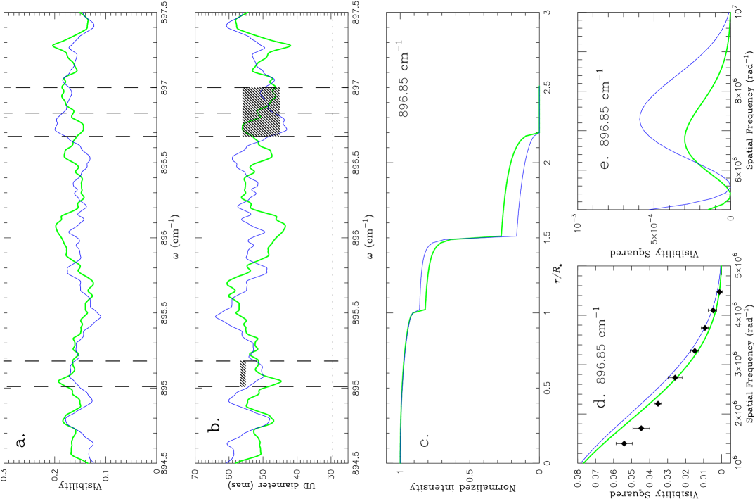
Figure 4: a: Visibilities calculated from the best-fit model for $o$ Cet in the 11 $\mu$m region for a projected baseline length of 30 m. In all the panels, the green solid lines represent results calculated with the HITEMP database, while the blue solid lines represent those calculated with the PS97 list. b: Uniform disk diameters calculated for a projected baseline length of 30 m. In a and b, the bandpasses used by WHT03a are marked with the dashed lines. The bandpasses used for the observations of $o$ Cet at around 896.83 cm^-1 lie between those shown (see WHT03a). The ranges of the uniform disk diameters measured in these bandpasses are shown as the hatched regions. The dotted line represents the photospheric angular diameter adopted in the calculation. A flux contribution of 70% from the dust shell is included in the calculations of the model visibilities, but not in the computation of the uniform disk diameters. Both plots (a and b) are redshifted by 0.248 cm^-1 with respect to the rest wavenumber, which corresponds to a radial velocity of 83 km s^-1, to match the observed spectrum shown in Fig. 2. c: The normalized intensity profile at 896.85 cm^-1, which is spectrally convolved with the same top-hat function as used in the calculation of the spectrally convolved visibility shown in a. d: The spectrally convolved squared visibilities at 896.85 cm^-1, plotted together with the visibility points observed by WHT03a (filled diamonds). e: The same spectrally convolved visibility squared as in d, but at higher spatial frequencies.

We now calculate the angular diameter of $o$ Cet predicted from the above model for the warm water vapor envelope. In order to compare with the observed uniform disk diameters, it is necessary to estimate the angular size of the star, which corresponds to $R_{\star}$. Woodruff et al. (woodruff04 (2004)) analyzed the $K$-band interferometric data of $o$ Cet obtained with VLTI/VINCI at phases from 0.13 to 0.40. They derived the Rosseland radius as well as the continuum radius at 1.04 $\mu$m at each phase by fitting the observed visibilities with theoretical ones predicted by dynamical model atmospheres, and found that the continuum diameter at 1.04 $\mu$m at phase 0.40 is 340 $R_{\sun}$, which corresponds to 29.5 mas (see Fig. 7 in Woodruff et al. woodruff04 (2004)). In the present calculation, we adopt this value as the diameter of the stellar disk. Figures 4a and 4b show the predicted visibilities and uniform disk diameters, using the HITEMP database and the PS97 line list. The visibilities as well as the uniform disk diameters shown in the figure are calculated for a projected baseline length of 30 m, which is approximately the mean of the baseline lengths used by W00, WHT03a, and WHT03b. The presence of the extended dust shell lowers the visibility by an amount equal to the fraction of the flux contribution of the dust shell, and therefore, the visibilities resulting from the stellar disk and the warm H₂O envelope are lowered by a factor of 0.3 to account for the flux contribution of the dust shell in this wavelength region. Note, however, that the uniform disk diameters are computed from the visibilities excluding the dust shell, because the effect of the presence of the dust shell is already taken into account in the determination of the uniform disk diameters by W00, WHT03a, and WHT03b. The bandpasses used in the ISI observations are marked with the dashed lines, and the ranges of the uniform disk diameters observed within these bandpasses are shown as the hatched regions.

Figure 4b demonstrates that the predicted uniform disk diameters in the bandpasses centered around 896.83 cm^-1 are in agreement with those observed. The ISI observations within these bandpasses were carried out at various phases between 0.92 and 0.36, and therefore, it should be kept in mind that the range of the observed angular diameters shown in the figure is affected by a variation of the angular diameter with phase. The uniform disk diameters predicted within the bandpass centered at 895.1 cm^-1 are systematically lower than the observed value of $55.88\pm 0.74$ mas. However, the ISI observation for this bandpass was carried out at phase 0.26, while the high-resolution TEXES spectrum of $o$ Cet, which we used for deriving the parameters of the water vapor envelope, was obtained at phase 0.36. Furthermore, WHT03a note that the uniform disk diameter of $o$ Cet measured at 11.1419 $\mu$m increased by 11% ($\sim$6 mas) from 2000 to 2001, which they attribute to the non-periodic variation in the angular size and/or asymmetries. Therefore, the difference between the predicted angular diameters within the bandpass centered at 895.1 cm^-1 and that observed can be attributed to the mismatch in phase as well as this non-periodic variation and/or asymmetries of the stellar disk and the warm water vapor envelope.

Figure 4c shows the intensity profiles predicted at 896.85 cm^-1, using the HITEMP database (green solid line) and the PS97 line list (blue solid line). The spectrally convolved squared visibilities at this wavenumber are plotted as a function of spatial frequency for both cases with the HITEMP database and the PS97 line list in Fig. 4d, together with the observed values for $o$ Cet, which were read off Fig. 1 of WHT03a. The figure reveals that the predicted squared visibilities are in agreement with those observed at spatial frequencies higher than $\sim\!2.6\times 10^{6}$ rad^-1, while the agreement is slightly poorer at lower spatial frequencies. However, this small discrepancy can be due to the variation of the observed angular diameter mentioned above, and therefore, is not regarded as serious disagreement. Contemporaneous spectroscopic and interferometric observations would be desirable for further constraining our model for the warm water vapor envelope. Figure 4e shows the predicted squared visibilities at higher spatial frequencies, which correspond to baselines as long as $\sim$100 m. Mid-infrared interferometric observations with such long baselines would also be useful for examining our model further.

We perform the same calculation for the two bandpasses in the regions around 10.8844 $\mu$m and 11.0856 $\mu$m. Within the bandpasses in these wavelength regions, strong emission and absorption features due to H₂O are observed, as shown in the upper two panels of Fig. 2. Figure 5 shows the uniform disk diameters calculated with the HITEMP database and the PS97 line list in these wavelength regions. The figure demonstrates that the observed uniform disk diameter within the bandpass at 918.56 cm^-1 can be well reproduced by our model, while the uniform disk diameters predicted within the bandpass at 902.0 cm^-1 are lower than the observed value. It should be noted, however, that the ISI observations for these bandpasses were carried out at phases different from the phase 0.36 at which the TEXES spectrum was obtained: phase 0.95 for the bandpass at 918.56 cm^-1  and phase 0.20 for the bandpass at 902.0 cm^-1. This mismatch in phase as well as the systematic increase of the angular size from 2000 to 2001 mentioned above introduces ambiguities in comparing the predicted and observed uniform disk diameters. Given these ambiguities, the agreement between the predicted and observed uniform disk diameters within the two bandpasses containing the strong H₂O features can also be regarded as fair.

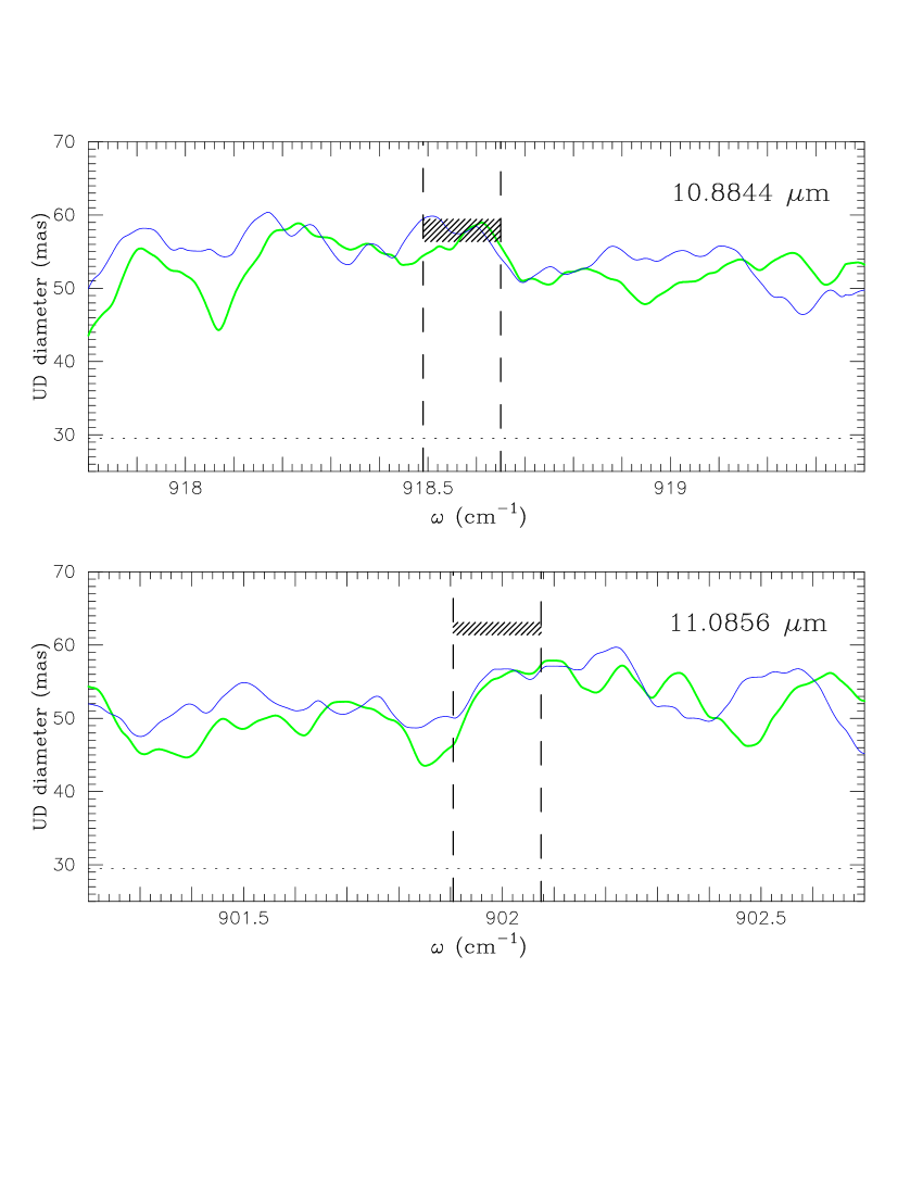
Figure 5: Uniform disk diameters around 10.8844 $\mu$m (upper panel) and 11.0856 $\mu$m (lower panel) calculated from the best-fit model for $o$ Cet for a projected baseline length of 30 m. In both panels, the green solid lines represent results calculated with the HITEMP database, while the blue solid lines represent those calculated with PS97 list. Both plots are redshifted by 0.248 cm^-1 in wavenumber, which corresponds to a radial velocity of 83 km s^-1, to match the observed spectrum shown in Fig. 2. The bandpasses used by WHT03a are marked with the dashed lines, and the ranges of the angular diameters measured by WHT03a are represented as the hatched regions. The dotted lines represent the photospheric angular diameter adopted in the calculation.

3.1.3 Near-infrared angular diameter

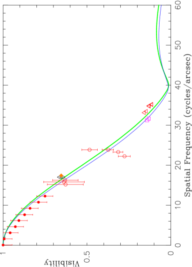
Figure 6: Comparison between the $K$-band visibilities observed for $o$ Cet and those predicted by the best-fit model for this object. The green solid line represents the visibility calculated with the HITEMP database, while the blue solid line represents that calculated with PS97 list. The observed visibilities include the results obtained by Ridgway et al. (ridgway92 (1992)) (phase 0.23–0.36, red open circles), the speckle data obtained at 0.26 by Woodruff et al. (woodruff04 (2004)) (red filled circles), and the VLTI/VINCI data obtained at phase 0.26 (red open triangles), 0.40 (purple open squares), 1.40 (black open diamonds), and 1.47 (orange filled diamonds).

We have shown that the high-resolution 11 $\mu$m  spectrum of $o$ Cet and its 11 $\mu$m angular diameter almost twice as large as those measured in the near-infrared can be reproduced by our model for the warm water vapor envelope. However, if the effect of the warm water vapor envelope on the near-infrared angular diameter is as large as that on the 11 $\mu$m angular diameter, our model may not reproduce the observed near-infrared visibilities and angular diameters of $o$ Cet. If it is the case, our model for the warm water vapor envelope as well as the photospheric angular diameter of 29.5 mas that we assumed based on the $K$-band VINCI observations may not be justified. Therefore, we calculate the visibility as well as the angular diameter of $o$ Cet in the near-infrared using the same best-fit model for $o$ Cet and compare with the observed values.

Although a number of near-infrared interferometric observations of $o$ Cet are presented in the literature, only a limited amount of data are available up to now for phases near 0.36. Given uncertainties in the determination of a zero point of pulsational phase, we can compare with data obtained at phases of approximately $0.36\pm 0.1$. Ridgway et al. (ridgway92 (1992)) obtained $K$-band visibilities between phase 0.23 and 0.36 with baseline lengths of 8 and 12 m. The $K$-band interferometric data of $o$ Cet presented by Woodruff et al. (woodruff04 (2004)) include data obtained at phases 0.26, 0.4, 1.4, and 1.47 (phases larger than 1 mean the next pulsation cycle), together with speckle interferometric data obtained with the 6 m telescope at the Special Astrophysical Observatory in Russia. The data obtained by Ridgway et al. (ridgway92 (1992)) as well as by Woodruff et al. (woodruff04 (2004)) were acquired with a broadband $K$ filter, which means that the derived apparent size is affected by molecular spectral features originating in the warm molecular envelope, in particular, H₂O lines located at the shorter and longer edges of the $K$ band. We calculate the uniform disk diameter in the $K$ band in almost the same manner as in the 11 $\mu$m region. The only difference is that we calculate the monochromatic visibility squared from the monochromatic intensity profile, and this monochromatic visibility squared is spectrally convolved for comparison with the above $K$-band visibility measurements. We include only H₂O lines in the calculation, and the $K$-band filter is approximated with a top-hat function centered at 2.2 $\mu$m with $\Delta\lambda$ = 0.4 $\mu$m. The $K$-band speckle visibility obtained at phase 0.26 shows no evidence of an extended dust shell, whose presence would result in a steep drop of visibility at low spatial frequencies (see Fig. 2 in Woodruff et al. woodruff04 (2004)). While a possible appearance of significant dust emission in the $K$ band at phases other than 0.26 cannot be ruled out, it seems to be unlikely that dust emission has a noticeable effect on the $K$-band visibility at phase 0.36. Therefore, no flux contribution from the dust shell is included in the calculation of visibilities in this wavelength region. Figure 6 shows a comparison between the observed $K$-band visibilities mentioned above and those predicted by the best-fit model for $o$ Cet. The figure illustrates that the observed visibilities are well reproduced by our model.

We also compare the predicted $K$-band uniform disk diameters with that observationally derived. From the predicted visibilities shown in Fig. 6, the uniform disk diameter is derived for a projected baseline length of 15 m, which is roughly the mean of the baselines used in the observations presented by Woodruff et al. (woodruff04 (2004)). The $K$-band uniform disk diameters predicted from the best-fit model for $o$ Cet are 34.1 mas with the HITEMP database and 34.9 mas with the PS97 line list. These predicted values are in agreement with the uniform disk diameter of $33.27\pm 0.33$ mas at phase 0.40 obtained by Woodruff et al (woodruff04 (2004)), and this agreement lends support to our model for the warm water vapor envelope as well as the photospheric angular diameter adopted in the present calculation.

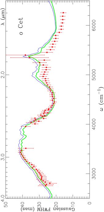
Figure 7: Wavelength dependence of the angular size (Gaussian FWHM) predicted from the best-fit model for $o$ Cet for a projected baseline length of 10 m. The red dots represent the angular size of $o$ Cet observed by Ireland et al. (ireland04 (2004)). The green solid line represents the result obtained with the HITEMP database, while the blue solid line represents that obtained with the PS97 line list. No flux contribution from the dust shell is included in the calculation shown.

Ireland et al. (ireland04 (2004)) measured the angular size of $o$ Cet in the near-infrared between 1.2 and 3.6 $\mu$m by aperture masking with the Keck telescope. The wavelength dependence of the angular size in the near-infrared appears to coincide with the wavelength dependence of the opacity of H₂O, which suggests that the observed near-infrared angular size may also be explained by our model for the warm water vapor envelope. We calculate the angular size, which is the Gaussian FWHM in this case, using the best-fit model for $o$ Cet, with only H₂O lines taken into account. The calculated visibility is convolved with a spectral resolution of 120, which approximately corresponds to the spectral resolution used for the Keck observations, and the Gaussian FWHM at each wavelength is derived for a projected baseline length of 10 m. Figure 7 shows a comparison between the angular sizes predicted from our best-fit model for $o$ Cet from 1.5 to 4.0 $\mu$m and that observed by Ireland et al. (ireland04 (2004)). The predicted angular sizes are in good agreement with the Keck observation, suggesting that the wavelength dependence of the angular size in the near-infrared largely reflects the opacity of H₂O lines. However, the Keck observation of $o$ Cet was carried out at phase 0.95, which is far from the phase 0.36 of the TEXES observation of $o$ Cet. Therefore, the apparent agreement between the observed and predicted near-infrared angular sizes of $o$ Cet  should be regarded as preliminary, and this highlights again the importance of coordinated spectroscopic and interferometric observations.

3.2 R Leo

3.2.1 11 $\mu$m and near-infrared spectra

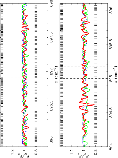
Figure 8: Spectra of R Leo in the 11 $\mu$m region at phase 0.75. The red dots represent the observed spectrum of R Leo presented in WHT03b, while the green and blue solid lines represent the calculated spectra using the HITEMP database and the PS97 line list, respectively. The parameters of the best-fit model for R Leo are $T_{\rm hot}$ = 2000 K, $R_{\rm hot}$ = 1.7 $R_{\star}$, $N_{\rm hot}$ = $1\times 10^{21}$ cm^-2, $T_{\rm cool}$ = 1200 K, $R_{\rm cool}$ = 2.2 $R_{\star}$, and $N_{\rm cool}$ = $7\times 10^{21}$ cm^-2. The synthetic spectra are convolved with a Gaussian with a FWHM of 0.013 cm^-1 to account for the effects of the instrument as well as of the macro-turbulent velocity, and are redshifted by 7 km s^-1 to match the observation. The dashed lines represent the bandpasses used in the ISI observations. The positions of the H₂O lines whose intensity at 2000 K is stronger than $1\times 10^{-24}$ cm molecule^-1 are marked with upper ticks (PS97 line list) and lower ticks (HITEMP database). These line positions are also redshifted by 7 km s^-1 with respect to the rest wavenumber.

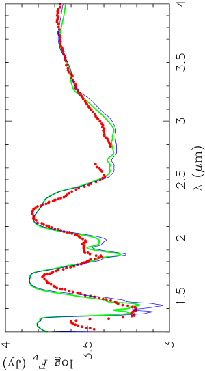
Figure 9: Spectra of R Leo in the region between 1.2 and 4.0 $\mu$m. The red dots represent the KAO spectrum of R Leo observed at phase 0.51 by Strecker et al. (strecker78 (1978)), while the green and blue solid lines represent the spectra from the best-fit model for phase 0.75, using the HITEMP database and the PS97 line list, respectively. The parameters of the model are given in the legend to Fig. 8. The synthetic spectra are convolved to match the spectral resolution of the KAO observation ($R\simeq 50$).

For R Leo, we find that the observed 11 $\mu$m spectrum and uniform disk diameters obtained by WHT03b can be best reproduced by a model with $T_{\rm hot}$ = 2000 K, $R_{\rm hot}$ = 1.7 $R_{\star}$, $N_{\rm hot}$ = $1\times 10^{21}$ cm^-2, $T_{\rm cool}$ = 1200 K, $R_{\rm cool}$ = 2.2 $R_{\star}$, and $N_{\rm cool}$ = $7\times 10^{21}$ cm^-2. Figure 8 shows the synthetic spectra in the 11 $\mu$m region predicted by the best-fit model for R Leo, together with the TEXES spectrum obtained at phase 0.75, which was read off Fig. 2 in WHT03b. The synthetic spectrum calculated with the HITEMP H₂O line list is represented with the green solid line, while that calculated with the PS97 H₂O line list is represented with the blue solid line. We estimated the flux contribution of the circumstellar dust shell in the 11 $\mu$m region based on the modeling of the spectral energy distribution (SED) and the visibility presented by Schuller et al. (schuller04 (2004)). Their model SED for R Leo, which can well reproduce the photometric observations in particular in the infrared, shows that the flux contribution of the dust shell at 11 $\mu$m is approximately 70% of the total flux (see Fig. 3 of Schuller et al. schuller04 (2004)), and we adopted $f_{\rm dust}=0.7$ in our calculation for R Leo. The synthetic spectra are redshifted by 7 km s^-1 to match the observation (see WHT03b). The figure shows that the synthetic spectra can reproduce the observed spectra without prominent spectral features in the bandpasses used for the ISI observations (marked with the dashed lines), which is a result of the filling-in effect due to the emission of the H₂O lines from the extended envelope. The approximate depths and heights of the observed fine spectral features are also reproduced, as in the case of $o$ Cet discussed above.

We also compare the predicted spectra in the near-infrared with that observed. For R Leo, the near-infrared spectrum obtained at phase 0.51 by Strecker et al. (strecker78 (1978)) using the Kuiper Airborne Observatory (KAO) would be the spectrum closest to that expected at phase 0.75, at which the high-resolution 11 $\mu$m  spectrum of R Leo was obtained. Figure 9 shows a comparison between the spectrum of R Leo observed by Strecker et al. (strecker78 (1978)) and those predicted from the best-fit model for R Leo, which are convolved to match the spectral resolution of 50 used by Strecker et al. (strecker78 (1978)). As we will see below, the $K$-band visibility observed with the Keck telescope (Monnier et al. monnier04 (2004)) does not show a steep drop at low spatial frequencies characteristic of an object with an extended dust shell. In addition, the SED modeling of Schuller et al. (schuller04 (2004)) shows that the flux contribution of the dust shell is $\sim$3% at most in the near-infrared ($\lambda\la 4$ $\mu$m). Therefore, the flux contribution of the dust shell is neglected in the calculation of the synthetic spectra. A glance of Fig. 9 reveals that the observed spectrum can be reasonably reproduced by the best-fit model for R Leo for phase 0.75, and the difference between the observed and predicted spectra might be attributed to the mismatch in phase between the observation and the model.

3.2.2 Angular diameters measured at 11 $\mu$m and in the near-infrared

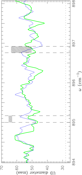
Figure 10: Uniform disk diameters calculated from the best-fit model for R Leo in the 11 $\mu$m region for a projected baseline length of 30 m. The green solid line represents the result calculated with the HITEMP database, while the blue solid line represents that calculated with the PS97 line list. The bandpasses used by WHT03b are marked with the dashed lines. The ranges of the diameters measured in these bandpasses are shown as the hatched regions. The dotted line represents the photospheric angular diameter adopted in the calculation. The calculated uniform disk diameters are redshifted by 0.021 cm^-1 with respect to the rest wavenumber, which corresponds to a radial velocity of 7 km s^-1, to match the observed spectrum shown in Fig. 8.

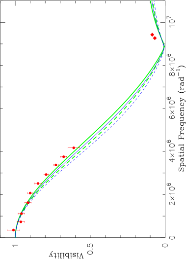
Figure 11: Comparison between the $K$-band visibilities of R Leo observed by Monnier et al. (monnier04 (2004)) and those predicted by the best-fit model for this object. The red filled circles represent the Keck observation, while the red filled diamonds represent the IOTA observation. The predicted visibilities which are convolved with a spectral resolution of 43 to match the Keck observation are plotted by the green solid line (calculated with the HITEMP database) and the blue solid line (calculated with the PS97 line list). The dashed lines represent the visibilities convolved with a spectral resolution of 7 to match the IOTA observation. The result calculated with the HITEMP database is plotted by the green dashed line, while that calculated with the PS97 line list is plotted by the blue dashed line.

We now compare the 11 $\mu$m angular diameters predicted from our model for R Leo with those obtained by the ISI observations. Figure 10 shows a comparison between the observed uniform disk diameters and those predicted from the best-fit model for R Leo. We tentatively adopt a photospheric angular diameter of 28 mas based on the measurements carried out at phase 0.24–0.28 by Perrin et al. (perrin99 (1999)) and examine the validity of this assumption by comparing with observed angular sizes in the near-infrared below. The uniform disk diameters are calculated from the visibilities excluding the dust shell for a projected baseline length of 30 m, as in the case of $o$ Cet. Figure 10 illustrates that the uniform disk diameters predicted within the bandpass at around 896.85 cm^-1 are in agreement with those measured with ISI. However, two measurements within this bandpass were carried out at different epochs and phases, and therefore, it is necessary to compare the model predictions with the observations carried out at similar phases to that at the time of the TEXES observation of R Leo.

The ISI observations were carried out in 1999 October (phase 0.43) and in 2001 October and November (phase 0.77) for the bandpass at 896.85 cm^-1 and in 2001 November (phase 0.81) for the bandpass at 895.1 cm^-1. Since our model for R Leo is based on the fitting to the TEXES spectrum obtained in 2000 December at phase 0.75, the predicted uniform disk diameters should be close to the values observed at similar phases, that is, $62.62\pm 1.14$ mas at 896.85 cm^-1 at phase 0.77 and $64.24\pm 1.12$ mas at 895.1 cm^-1 at phase 0.81. Although the predicted uniform disk diameters in the two bandpasses are somewhat smaller than these observed values obtained at phases close to 0.75, this difference may be attributed to a cycle-to-cycle variation and/or deviation from circular symmetry as WHT03a discuss for $o$ Cet. Given such a possible temporal variation of the angular size and a presence of asymmetries, we can conclude that our model for the warm water vapor envelope can fairly reproduce the observed 11 $\mu$m uniform disk diameter of R Leo.

As in the case of $o$ Cet, we compare near-infrared visibilities predicted by the best-fit model for R Leo with those observed at phases close to 0.75. Monnier et al. (monnier04 (2004)) have recently combined interferometric data from Keck aperture masking and the Infrared Optical Telescope Array (IOTA) for ten objects including R Leo. They observed R Leo at phase 0.7, very close to the phase 0.75. Figure 11 shows a comparison between the $K$-band visibilities obtained by Monnier et al. (monnier04 (2004)) and those predicted from the best-fit model for R Leo. The observed visibility at low spatial frequencies ($\la 4\times 10^{6}$ rad^-1) does not show a sharp drop, which would be present if there were flux contribution from the dust shell. Therefore, we include no dust emission in the calculation of the $K$-band visibilities. The predicted visibilities are spectrally convolved with a Gaussian with a FWHM of 0.053 $\mu$m ($R\simeq 43$) to match the width of the narrow-band filter used for the Keck observation. For comparison with the IOTA data, which were obtained with a broadband $K^{\prime}$ filter, the predicted visibilities are convolved with a top-hat function centered at 2.16 $\mu$m with $\Delta\lambda=0.32$ $\mu$m ($R\simeq 7$). Figure 11 demonstrates that the visibility obtained by Keck aperture masking (red filled circles) can be well reproduced by the best-fit model, while the predicted visibilities are too low compared to the visibility points obtained with IOTA (red filled diamonds). This discrepancy at high spatial frequencies may be attributed to the simplicity of our model and/or a cycle-to-cycle variation which might have taken place between the Keck+IOTA observations (2000 January and February) and the TEXES observation (2000 December).

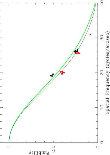
Figure 12: Comparison between the $L^{\prime}$ -band visibilities of R Leo observed by Chagnon et al. (chagnon02 (2002)) and those predicted by the best-fit model for this object. The black filled circles represent the visibilities observed in 2000 March (phase 0.81–0.82), while the red filled circles represent those observed in 2000 November (phase 0.61–0.64). The green solid line represents the predicted visibility calculated with the HITEMP database, while the blue solid line represents that calculated with the PS97 line list.

Chagnon et al. (chagnon02 (2002)) measured $L^{\prime}$-band visibility of R Leo at two epochs, phase $\sim$0.6 and $\sim$0.8, both of which are rather close to the phase 0.75. Figure 12 shows a comparison between the observed $L^{\prime}$-band visibilities of R Leo and those predicted by the best-fit model for this object. Since the flux contribution of the dust shell is expected to be $\sim$3% at most in the $L^{\prime}$ band as mentioned above, no flux contribution from the dust shell is included in the calculation of the $L^{\prime}$-band visibilities. The predicted visibilities are spectrally convolved with a top-hat function centered at 3.8 $\mu$m with $\Delta\lambda$ = 0.54 $\mu$m to match the observed data. The figure illustrates that the observed visibilities can be fairly reproduced by our model, given the slight mismatch in phase as well as a possible cycle-to-cycle variation of the warm water vapor envelope. This agreement of the $L^{\prime}$-band visibility lends further support to the photospheric angular diameter that we adopted and our basic picture of the warm water vapor envelope.

We also compare the wavelength dependence of the angular size predicted in the near-infrared with that observed by Ireland et al. (ireland04 (2004)). Their observation of R Leo in the wavelength region between 1.2 and 3.6 $\mu$m with the Keck telescope was carried out at phase 0.74, which is very close to the phase of 0.75 at which the high-resolution 11 $\mu$m  spectrum was obtained. We calculate the near-infrared angular size using the best-fit model for R Leo  in the same manner as in the case of $o$ Cet. Comparison between the observed Gaussian FWHM of R Leo and those predicted from our model shown in Fig. 13 illustrates that our model can reproduce the observed Gaussian FWHM from 1.5 to 3.6 $\mu$m quite well. This agreement of the near-infrared angular size of R Leo suggests again that the H₂O lines govern the wavelength dependency of the angular size of Mira variables in this wavelength regime.

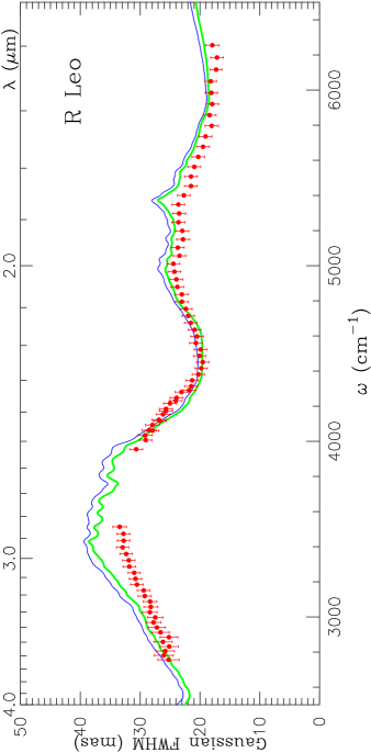
Figure 13: Wavelength dependence of the angular size (Gaussian FWHM) predicted from the best-fit model for R Leo for a projected baseline length of 10 m. The red dots represent the angular size of R Leo observed by Ireland et al. (ireland04 (2004)). The green solid line represents the result obtained with the HITEMP database, while the blue solid line represents the result with the PS97 line list. No flux contribution from the dust shell is included in the calculation shown.

3.3 $\chi$ Cyg

3.3.1 11 $\mu$m and near-infrared spectra

For $\chi$ Cyg, we find that the observed 11 $\mu$m spectrum and the uniform disk diameter obtained by WHT03b can be best reproduced by a model with $T_{\rm hot}$ = 2000 K, $R_{\rm hot}$ = 1.5 $R_{\star}$, $N_{\rm hot}$ = $1\times 10^{21}$ cm^-2, $T_{\rm cool}$ = 1200 K, $R_{\rm cool}$ = 2.2 $R_{\star}$, and $N_{\rm cool}$ = $1\times 10^{21}$ cm^-2. Figure 14 shows a comparison between the TEXES spectrum of $\chi$ Cyg, which was obtained in 2001 mid-June at phase 0.4, and those predicted by the above best-fit model for this object. The flux contribution of the circumstellar dust shell at 11 $\mu$m was estimated from the visibility function at 11 $\mu$m obtained by Danchi et al. (danchi94 (1994)), which indicates a steep drop at low spatial frequencies resulting from the presence of the extended dust shell. The amount of the visibility drop, which is equal to the fraction of the flux contribution of the dust shell, is approximately 0.6, and we adopted $f_{\rm dust}=0.6$ in our calculation for $\chi$ Cyg. The synthetic spectra are blueshifted by 22 km s^-1 to match the observation (see WHT03b). Figure 14 demonstrates that the observed spectrum (red dots) can be well reproduced by the model. Like in the cases of $o$ Cet and R Leo discussed above, the filling-in effect due to H₂O line emission from the extended envelope leads to the featureless, continuum-like spectra.

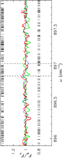
Figure 14: Spectra of $\chi$ Cyg in the 11 $\mu$m region at phase 0.4. The red dots represent the observed spectrum of $\chi$ Cyg presented in WHT03b, while the green and blue solid lines represent the calculated spectra using the HITEMP database and the PS97 line list, respectively. The parameters of the best-fit model for $\chi$ Cyg are $T_{\rm hot}$ = 2000 K, $R_{\rm hot}$ = 1.5 $R_{\star}$, $N_{\rm hot}$ = $1\times 10^{21}$ cm^-2, $T_{\rm cool}$ = 1200 K, $R_{\rm cool}$ = 2.2 $R_{\star}$, and $N_{\rm cool}$ = $1\times 10^{21}$ cm^-2. The synthetic spectra are convolved with a Gaussian with a FWHM of 0.013 cm^-1 to account for the effects of the instrument as well as of the macro-turbulent velocity, and are blueshifted by 22 km s^-1 to match the observation. The dashed lines represent the bandpasses used in the ISI observations. The positions of the H₂O lines whose intensity at 2000 K is stronger than $1\times 10^{-24}$ cm molecule^-1 are marked with upper ticks (PS97 line list) and lower ticks (HITEMP database). These line positions are also blueshifted by 22 km s^-1 with respect to the rest wavenumber.

The presence of such a dense water vapor envelope around $\chi$ Cyg, though the H₂O column density is smaller than that in $o$ Cet and R Leo, may appear to be in conflict with the classification of this object as an S star. S stars have C/O ratios close to unity, and therefore, neither oxygen-bearing nor carbon-bearing molecules are abundant in the atmosphere, with most of carbon and oxygen atoms locked up in CO molecules. In fact, the H₂O lines observed for $\chi$ Cyg in the 4 $\mu$m region are significantly weaker than those observed in oxygen-rich Miras (Lebzelter et al. lebzelter01 (2001)). However, there are some pieces of observational evidence for the presence of a significant amount of water vapor in $\chi$ Cyg near minimum light. Based on the H₂O absorption features in the 9000 Å region, Spinrad & Vardya (spinrad66b (1966)) estimated the H₂O column density in $\chi$ Cyg to be $3\times 10^{21}$ cm^-2 at minimum light, which is in agreement with the result we obtained above. Wallace & Hinkle (wallace97 (1997)) present a series of $K$-band spectra of $\chi$ Cyg observed at various phases with a spectral resolution of $\sim$3000 using a Fourier Transform Spectrometer (FTS), and the spectra exhibit an increasing absorption in the region between $\sim$4700 cm^-1 and 4950 cm^-1 from maximum light (phase 0.00) to minimum light (phase 0.42–0.48). Figure 15a shows the spectra acquired at phase 0.00 and 0.42, and the thick red solid line in Fig. 15b represents the ratio of these two spectra (i.e., spectrum at 0.42 divided by spectrum at 0.00). This ratioed spectrum clearly shows the enhanced absorption which appears between $\sim$4700 and 4950 cm^-1 near minimum light. The thin green solid line in Fig. 15b represents the H₂O spectrum predicted by the above best-fit model for $\chi$ Cyg using the HITEMP database. Dyck et al. (dyck84 (1984)) estimated that more than 90% of the observed flux between 2.2 and 4.8 $\mu$m comes from the star based on the modeling of Rowan-Robinson & Harris (rowanrobinson83 (1983)). Therefore, the flux contribution of the dust shell is not included in the calculation of the synthetic spectrum. As the figure shows, the absorption observed between $\sim$4700 and 4950 cm^-1 is reproduced by the synthetic spectrum, and the individual absorption features seen in the ratioed spectrum can be identified as H₂O lines, whose line positions are marked with the ticks in the figure.

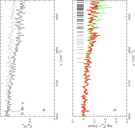
Figure 15: Spectra of $\chi$ Cyg in the region between 4600 and 4950 cm^-1. a: The dotted line represents the spectrum of $\chi$ Cyg obtained at phase 0.00, while the solid line represents the spectrum at phase 0.42 (Wallace & Hinkle wallace97 (1997)). b: The thick red solid line represents the ratio between the spectra observed at phase 0.00 and 0.42. The thin green solid line represents the spectrum predicted by the best-fit model for $\chi$ Cyg, whose parameters are given in the legend to Fig. 14. The synthetic spectrum is convolved to match the spectral resolution of $R\simeq 3000$ used in the observations by Wallace & Hinkle (wallace97 (1997)).

Finally, more definitive evidence for the presence of a large amount of water vapor in $\chi$ Cyg near minimum light can be found in the near-infrared spectrum obtained with ISO/SWS. Vandenbussche et al. (vandenbussche02 (2002)) present the ISO/SWS spectrum of $\chi$ Cyg obtained on 1998 May 10 (UT 07:39:48) at phase 0.5 in the wavelength region between 2.3 and 4.1 $\mu$m. We retrieved this ISO/SWS spectrum of $\chi$ Cyg from the ISO data archive and plot it in Fig. 16. The spectrum clearly exhibits the absorption feature centered at 2.7 $\mu$m due to the H₂O $\nu_{1}$ and $\nu_{3}$ fundamental bands. Also plotted in the figure are the spectra predicted from the above best-fit model for $\chi$ Cyg, and the figure demonstrates that the predicted spectra are in fair agreement with that observed, given the simplicity of our model as well as a slight mismatch in phase between the TEXES observation and the ISO/SWS observation.

The above observational results show that water vapor is present in the S-type Mira variable $\chi$ Cyg near minimum light, and that the amount of water vapor is comparable to those found in the oxygen-rich Miras $o$ Cet and R Leo. In general, Mira variables exhibit the strongest molecular absorption near minimum light (e.g., Lançon & Wood lancon00 (2000)), which implies that the temperature may be the lowest at minimum light and that the formation of water vapor may be significantly promoted at such low temperatures. However, detailed calculations using dynamical atmospheres are necessary for understanding the formation of H₂O in Mira variables with C/O ratios very close to unity.

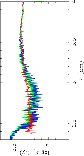
Figure 16: Spectra of $\chi$ Cyg in the region between 2.3 and 4.0 $\mu$m. The red solid line represents the spectrum of $\chi$ Cyg obtained at phase 0.5 with ISO/SWS (Vandenbussche et al. vandenbussche02 (2002)), while the green and blue solid lines represent the spectra from the best-fit model for phase 0.4, using the HITEMP database and the PS97 line list, respectively. The parameters of the model are given in the legend to Fig. 14. The synthetic spectra are convolved to match the spectral resolution of the ISO/SWS observation ($R\simeq 1500$), and no flux contribution from the dust shell is included.

3.3.2 Angular diameters measured at 11 $\mu$m and in the near-infrared

In Fig. 17, we compare the angular diameter of $\chi$ Cyg measured in the 11 $\mu$m region and those predicted by the above best-fit model for this object. The phase of $\chi$ Cyg at the time of the ISI observation is 0.51 (2001 July and August, see WHT03b), which is quite close to the phase 0.4 at which the TEXES spectrum was obtained. We adopt a photospheric angular diameter of 23 mas based on a $K^{\prime}$-band uniform disk diameter measured by Mennesson et al. (mennesson02 (2002)) at phase 0.38, which is also close to the phase 0.4. As in the cases of $o$ Cet and R Leo, we check the validity of the assumed photospheric angular diameter by calculating the near-infrared angular diameters below. The uniform disk diameters are calculated from the visibilities excluding the dust shell for a projected baseline length of 30 m. Figure 17 shows that the uniform disk diameters predicted in the ISI bandpass are in agreement with the observed value of $39.38\pm 4.02$ mas.

We also compare the angular diameters predicted in the near-infrared with those observed. Mennesson et al. (mennesson02 (2002)) observed $\chi$ Cyg in the $K^{\prime}$ and $L^{\prime}$ bands and derived uniform disk diameters of $23.24\pm 0.08$ mas and $30.40^{+3.30}_{-7.28}$ mas, respectively. We calculate the uniform disk diameters in these bands, with the $K^{\prime}$- and $L^{\prime}$-band filters represented with top-hat functions centered at 2.16 $\mu$m with $\Delta\lambda$ = 0.32 $\mu$m and at 3.8 $\mu$m with $\Delta\lambda$ = 0.54 $\mu$m, respectively. The $K^{\prime}$-band uniform disk diameters calculated with the HITEMP database and the PS97 line list for a projected baseline length of 20 m are 24.4 mas and 24.7 mas, respectively. These predicted $K^{\prime}$-band uniform disk diameters are in reasonable agreement with the observed value, which was measured at phase 0.38, very close to the phase 0.4 of the TEXES observation. The $L^{\prime}$-band uniform disk diameters calculated with the HITEMP database and the PS97 line list are 27.1 mas and 28.1 mas, respectively. While these predicted $L^{\prime}$-band uniform disk diameters are also in agreement with the observed one within the error of the measurement, it should be noted that the $L^{\prime}$-band observations of Mennesson et al. (mennesson02 (2002)) were carried out at phase 0.81, which makes it difficult to compare the observed angular diameter with that predicted by the best-fit model based on the TEXES spectrum obtained at phase 0.4. Therefore, we can conclude that the near-infrared angular diameters predicted by our model for $\chi$ Cyg are in rough agreement with those observed, while more rigorous tests are necessary using contemporaneous interferometric observations in the near-infrared and in the mid-infrared.

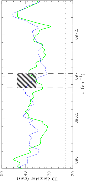
Figure 17: Uniform disk diameters calculated from the best-fit model for $\chi$ Cyg in the 11 $\mu$m region for a projected baseline length of 30 m. The green solid line represents the result obtained with the HITEMP database, while the blue solid line represents the result with the PS97 line list. The bandpass used by WHT03b is marked with the dashed lines. The range of the diameters measured in this bandpass is shown as the hatched region. The dotted line represents the photospheric angular diameter adopted in the calculation. The calculated uniform disk diameters are blueshifted by 0.0658 cm^-1 with respect to the rest wavenumber, which corresponds to a radial velocity of $-22$ km s^-1, to match the observed spectrum shown in Fig. 14.

4 Discussion

Our two-layer model for the warm water vapor envelope around three Mira variables can reproduce the observed increase of the angular diameter from the near-infrared to the 11 $\mu$m region and, simultaneously, the observed high-resolution 11 $\mu$m spectra which appear to be featureless. It is obvious, however, that our ad hoc model is not a unique solution, and that physical processes responsible for the formation of such warm water vapor layers also remain to be theoretically understood.

Intensity profiles predicted by dynamical model atmospheres for Mira variables exhibit structures consisting of two components. Tej et al. (tej03 (2003)) show that the formation of H₂O layers behind shock fronts leads to intensity profiles consisting of a step-like structure close to the star and/or a tenuous halo-like structure extending to a few stellar radii. The intensity profiles predicted by our models for the three Mira variables studied here also show such a step-like structure and a more extended component, as can be seen in Fig. 4c. This implies the possibility that the large-amplitude pulsation in Mira variables is responsible for the warm molecular envelope in these objects, and the next logical step would be to calculate synthetic spectra as well as intensity profiles using dynamical model atmospheres such as presented in Tej et al. (tej03 (2003)) and extensive H₂O line lists.

Hinkle & Barnes (hinkle79 (1979)) analyzed H₂O lines in high-resolution near-infrared spectra (4000–6700 cm^-1) of R Leo and identified two distinct H₂O layers, that is, a warm component with a temperature of $\sim$1700 K and a cool component with a temperature of $\sim$1100 K. This result seems to be in agreement with the temperatures of the H₂O layers we obtained for R Leo in the present work. The H₂O column densities of the cool component derived by Hinkle & Barnes (hinkle79 (1979)) range from $10^{21}$–$10^{22}$ cm^-2, and these values also agree with the $7\times 10^{21}$ cm^-2 we derived for the cool H₂O  layer. On the other hand, the H₂O column densities of the warm component they derived are $10^{19}$–$10^{20}$ cm^-2, which are significantly smaller than the $1\times 10^{21}$ cm^-2 derived here. Hinkle & Barnes (hinkle79 (1979)) also note that the H₂O lines originating in the warm component are never predominant compared to those originating in the cool component, which shows a marked contrast to our result that the hot H₂O layer contributes significantly in the spectrum as well as in the intensity profile. However, Hinkle & Barnes (hinkle79 (1979)) derived the H₂O column densities at phases 0.94, 0.00, 0.14, and 0.20, but not at phases between 0.5 and 0.9 because of the blend of H₂O lines originating in the two components. Since our model for R Leo is based on the TEXES spectrum obtained at phase 0.75, the above discrepancy of the H₂O column density of the warm component might be due to the mismatch in phase. Comparison with synthetic spectra using dynamical model atmospheres would be necessary to derive physical parameters such as excitation temperature and column density from the high-resolution spectra observed near minimum light which are severely affected by the blend of lines.

5 Concluding remarks

We have shown that our two-layer model for the warm water vapor envelope around the Mira variables $o$ Cet, R Leo, and $\chi$ Cyg can reproduce the observed increase of the angular diameter from the near-infrared to the 11 $\mu$m region and, simultaneously, the observed high-resolution 11 $\mu$m  spectra. While a number of H₂O pure rotation lines are present in the wavelength region observed with ISI and strong absorption can be expected, the absorption lines are filled in by the emission lines originating in the extended part of the water vapor envelope, which leads to the featureless, continuum-like spectra. This filling-in effect masks the spectroscopic fingerprints of the warm water vapor envelope, but its presence manifests itself as an increase of the angular diameter from the near-infrared to the mid-infrared: invisible for spectrometers but not for interferometers. The radii, temperatures, and H₂O column densities of the hot H₂O layer in the three Mira variables studied here are derived to be 1.5–1.7 $R_{\star}$, 1800–2000 K, and (1–$5)\times 10^{21}$ cm^-2, respectively. The cool H₂O layer is found to have temperatures of 1200–1400 K, extending to 2.2–2.5 $R_{\star}$ with H₂O column densities of (1–$7)\times 10^{21}$ cm^-2. Our models which reproduce the spectra and angular diameters observed at 11 $\mu$m have turned out to also reproduce the spectra and the visibilities as well as the angular diameters observed in the near-infrared. Comparison between the near-infrared angular sizes predicted for $o$ Cet as well as for R Leo and those observed with the Keck telescope suggests that the wavelength dependence of the angular size of Mira variables in the near-infrared largely reflects the H₂O  opacity.

We have also found evidence for the presence of a large amount of water vapor in $\chi$ Cyg near minimum light in the FTS spectra obtained in the $K$ band as well as in the ISO/SWS spectrum between 2.3 and 4.1 $\mu$m. The observed H₂O absorption features can be reasonably well reproduced by our water vapor envelope model whose parameters are derived from the comparison of the spectrum and the angular diameter observed at 11 $\mu$m. While S-type Miras are known to exhibit significantly weak spectral features due to oxygen-bearing molecules compared to oxygen-rich Miras, water vapor of an amount comparable to that in oxygen-rich Miras is present in $\chi$ Cyg near minimum light.

In order to test our model for the warm water vapor envelope further, contemporaneous spectroscopic and interferometric observations are indispensable, given the variations of the spectra and the angular size not only with phase but also on a time scale longer than the variability period. ISI observations using many more bandpasses in the 11 $\mu$m region and/or with even higher spectral resolution would also be useful for this purpose.

- (1) Cami, J., Yamamura, I., de Jong, T., et al. 2000, A&A, 360, 562
- (2) Chagnon, G., Mennesson, B., Perrin, G., et al. 2002, AJ, 124, 2821
- (3) Danchi, W. C., Bester, M., Degiacomi, C. G., Greenhill, L. J., & Townes, C. H. 1994, AJ, 107, 1469
- (4) Dyck, H. M., Zuckerman, B., Leinert Ch., & Beckwith, S. 1984, ApJ, 287, 801
- (5) Hinkle, K. H., & Barnes, T. G. 1979, ApJ, 227, 923
- (6) Ireland, M., Tuthill, P., Robertson, G., et al. 2004, In: Variable Stars in the Local Group, eds. D. W. Kurtz & K. Pollard, ASP. Conf. Series, in press
- (7) Lacy, J. H., Richter, M. J., Greathouse, T. K., Jaffe, D. T., & Zhu, Q. 2002, PASP, 114, 153
- (8) Lançon, A., & Wood, P. R. 2000, A&AS, 146, 217
- (9) Lebzelter, T., Hinkle, K. H., & Aringer, B. 2001, A&A, 377, 617
- (10) Matsuura, M., Yamamura, I., Cami, J., Onaka, T., & Murakami, H. 2002, A&A, 383, 972
- (11) Mennesson, B., Perrin, G., Chagnon, G., et al. 2002, ApJ, 579, 446
- (12) Monnier, J. D., Millan-Gabet, R., Tuthill, P. G., et al. 2004, ApJ, 605, 436
- (13) Ohnaka, K. 2004, A&A, 421, 1149 (Paper I)
- (14) Partridge, H., & Schwenke, D. W. 1997, J. Chem. Phys., 106, 4618
- (15) Perrin, G., Coudé du Foresto, V., Ridgway, S. T., et al. 1999, A&A, 345, 221
- (16) Perrin, G., Ridgway, S. T., Coudé du Foresto, V., et al. 2004, A&A, 418, 675
- (17) Ridgway, S. T., Benson, J. A., Dyck, H. M., Townsley, L. K., & Hermann, R. A. 1992, AJ, 104, 2224
- (18) Rothman, L. S. 1997, HITEMP CD-ROM (Andover: ONTAR Co.)
- (19) Rowan-Robinson, M., & Harris, S. 1983, MNRAS, 202, 767
- (20) Ryde, N., Lambert, D. L., Richter, M. J., & Lacy, J. H. 2002, ApJ, 580, 447
- (21) Schuller, P., Salomé, P., Perrin, G., et al. 2004, A&A, 418, 151
- (22) Spinrad, H., & Vardya, M. S. 1966, ApJ, 146, 399
- (23) Strecker, D. W., Erickson, E. F., & Witteborn, F. C. 1978, AJ, 83, 26
- (24) Tej, A., Lançon, A., & Scholz, M. 2003, A&A, 401, 347
- (25) Tsuji, T. 1978, A&A, 68, L23
- (26) Tsuji, T. 1986, A&A, 156, 8
- (27) Tsuji, T. 1988, A&A, 197, 185
- (28) Tsuji, T., Ohnaka K., Aoki, W., & Yamamura, I. 1997, A&A, 320, L1
- (29) van Belle, G. T., Dyck, H. M., Benson, J. A., & Lacasse, M. G. 1996, AJ, 112, 2147
- (30) Vandenbussche, B., Beintema, D., de Graauw, T., et al. 2002, A&A, 390, 1033
- (31) Wallace, L., & Hinkle, K. 1997, ApJS, 111, 445
- (32) Weiner, J., Danchi, W. C., Hale, D. D. S., et al. 2000, ApJ, 544, 1097 (W00)
- (33) Weiner, J., Hale, D. D. S., & Townes, C. H. 2003a, ApJ 588, 1064 (WHT03a)
- (34) Weiner, J., Hale, D. D. S., & Townes, C. H. 2003b, ApJ 589, 976 (WHT03b)
- (35) Woodruff, C., Eberhardt, M., Driebe, T., et al. 2004, A&A, 421, 703
- (36) Yamamura, I., de Jong, T., & Cami, J. 1999, A&A, 348, L55