On using visibility correlations to probe the HI distribution from the dark ages to the present epoch I: Formalism and the expected signal

Abstract

Redshifted 21 cm radiation originating from the cosmological distribution of neutral hydrogen (HI) appears as a background radiation in low frequency radio observations. The angular and frequency domain fluctuations in this radiation carry information about cosmological structure formation. We propose that correlations between visibilities measured at different baselines and frequencies in radio-interferometric observations be used to quantify the statistical properties of these fluctuations. This has an inherent advantage over other statistical estimators in that it deals directly with the visibilities which are the primary quantities measured in radio-interferometric observations. Also, the visibility correlation has a very simple relation with the power spectrum. We present estimates of the expected signal for nearly the entire post-recombination era, from the dark ages to the present epoch. The epoch of reionization, where the HI has a patchy distribution, has a distinct signature where the signal is determined by the size of the discrete ionized regions. The signal at other epochs, where the HI follows the dark matter, is determined largely by the power spectrum of dark matter fluctuations. The signal is strongest for baselines where the antenna separations are within a few hundred times the wavelength of observation, and an optimal strategy would preferentially sample these baselines. In the frequency domain, for most baselines the visibilities at two different frequencies are uncorrelated beyond $\Delta\nu\sim 1\,{\rm MHz}$, a signature which in principle would allow the HI signal to be easily distinguished from the continuum sources of contamination.

1 Introduction

One of the major problems in modern cosmology is to determine the distribution of matter on large scales in the universe and understand the large scale structure (LSS) formation . The last decade has witnessed phenomenal progress, particularly on the observational front where CMBR anisotropies (eg. Spergel et al. 2003) and galaxy redshift surveys (eg. Tegmark et al. 2003a, 2003b) in conjunction with other observations have determined the parameters of the background cosmological model and the power spectrum of density fluctuations to a high level of precision. These observations are all found to be consistent with a $\Lambda$CDM cosmological model with a scale invariant primordial power spectrum, though there are hints of what could prove to be very interesting features beyond the simplest model.

Another very interesting problem, on smaller scales in cosmology, is the formation of the first gravitationally bound objects and their subsequent merger to produce galaxies. Observations of quasar spectra show the diffuse gas in the universe to be completely ionized at redshifts $z\leq 5$ (Fan et al., 2002). Understanding the reionization process and its relation with the first generation of luminous objects produced by gravitational collapse is one of the challenges facing modern cosmology.

Observations of the redshifted 21 cm HI radiation provide an unique opportunity for probing the universe from the dark ages when the hydrogen gas first decoupled from the CMBR to the present epoch. Such observations will allow us to probe in detail how the universe was reionized. In addition, redshifted HI observations will allow the large scale distribution of matter in the universe to be studies over a very wide range of redshifts. The possibility of observing 21 cm emission from the cosmological structure formation was first recognized by Sunyaev and Zeldovich (1972). Later studies by Hogan & Rees (1979) and Scott & Rees (1990) consider both emission and absorption against the CMBR.

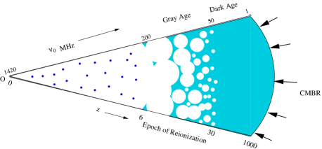
Figure 1: This figure schematically shows the evolution of HI (shaded in the figure) through the entire history of the universe. Hydrogen decouples from the CMBR at $z\sim 1000$ when electrons and protons combine, for the first time, to produce HI. The subsequent era, until the formation of the first luminous objects at $z\sim 30$, is referred to as the dark ages or the Pre-reionization era. The HI, in this era, is nearly uniformly distributed with small fluctuations which trace the dark matter. The first luminous objects reionize the HI. The reionization is initially confined to small bubbles surrounding the luminous objects. The bubbles of ionized HII gas grow until they finally overlap and the whole universe is reionized by $z\sim 6$. The HI distribution in the Reionization era or the Gray Age is patchy. Only the HI in dense collapsed objects survive the reionization. The surviving HI clouds which are seen as DLAs in quasar absorption spectra are shown as points in the figure. The large scale distribution of these clouds is assumed to follow the dark matter. Also shown is the CMBR which propagates through the intervening HI to the observer at $z=0$.

The cosmological evolution of the HI gas is shown schematically in Figure 1. The 21 cm emission has been perceived as a very important tool for studying the epoch of reionization, and the expected signature, in 21 cm, of the heating of the HI gas and its subsequent reionization has been studied extensively (Madau, Meiksin & Rees 1997; Gnedin & Ostriker 1997; Shaver et al. 1999; Tozzi et al. 2000; Iliev et al. 2002; Iliev et al. 2003; Ciardi & Madau 2003; Furlanetto,Sokasian. & Hernquist 2003; Gnedin & Shaver 2003; Miralda-Escude 2003; Chen & Miralda-Escude 2004). The timing, duration and character of the events which led to the reionization of the universe contains an enormous amount of information about the first cosmic structures and also has important implication for the later generations of baryonic objects. This process is not very well understood (eg. Barkana & Loeb 2001), but there are several relevant observational constraints.

The observation of quasars at redshift $z\sim 6$ which show strong HI absorption (Becker et al., 2001) indicates that at least $1\%$ of the total hydrogen mass at $z\sim 6$ is neutral (Fan et al., 2002), and the neutral mass fraction decreases rapidly at lower redshifts. This is a strong indication that the epoch of reionization ended at $z\sim 6$ .

Observations of the CMBR polarization, generated through Thomson scattering of CMBR photons by free electrons along the line of sight, indicates that the reionization began at a redshift $z>14$. On the other hand, the observed anisotropies of the CMBR indicate that the total optical depth of the Thomson scattering is not extremely high, suggesting that reionization could not have started at redshift much higher than about 30 ((Spergel et al., 2003).

A third constraint comes from determinations of the IGM temperature from observations of the ${\rm Ly}\alpha$ forest in the $z$ range $2$ to $4$ which indicates a complex reionization history with there possibly being an order unity change in the neutral hydrogen fraction at $z\leq 10$ (Theuns et al. 2002; Hui & Haiman 2003).

The possibility of observing the HI emission at $z\leq 6$, the post-reionization era, has also been discussed extensively particularly in the context of the Giant Meterwave Radio Telescope (GMRT) (Subramanian & Padmanabhan 1993; Kumar, Padmanabhan & Subramanian 1985; Bagla, Nath and Padmanabhan 1997; Bharadwaj, Nath & Sethi 2001; Bagla & White 2002). These observations will probe the large scale structure formation at the redshift where the HI emission originated.

Loeb & Zaldarriaga (2003) have recently proposed that observations of the angular fluctuations in the HI absorptions against the CMBR, originating in the $z$ range $30$ to $200$ corresponding to the dark age of the universe, would allow the primordial power spectrum to be probed at an unprecedented level of accuracy. Bharadwaj & Ali (2004) have investigated this in detail including the effect of redshift space distortion and gas temperature fluctuations.

In this paper we discuss the nature and the magnitude of the HI signal expected across the entire redshift range starting from the dark age of the universe at $z\sim 1000$ through the epoch of reionization to the present era. Our discussion is in the context of observations using radio interferometric arrays to study the redshifted HI signal. Such observations are sensitive to only the angular fluctuations in the HI signal. The quantity measured in radio interferometric observations is the complex visibility. Typically, the visibilities are used to construct an image which is then analysed. An image of the HI distribution, while interesting, is not the optimal tool for quantifying and analysing the redshifted HI radiation. The quantities of interest are the statistical properties of the fluctuations in the redshifted HI radiation, and an image, if at all useful, is only an intermediate step in the process of extracting these statistical quantities. Here we propose that correlations between the complex visibilities measured at different baselines and frequencies be used to directly quantify the angular and frequency domain clustering pattern in the HI radiation, completely doing away with the need for making an image.

In Section 2 of this paper we develop the formalism for calculating visibility correlations, bringing out the relation between this quantity and various properties of the HI distribution. The fluctuations, with angle and frequency, of the redshifted HI radiation can be directly related to fluctuations in the properties of the HI distribution in space. The mapping is a little complicated due to the presence of peculiar velocities which moves around spectral features along the frequency direction. This effect, not included in most earlier calculations, is very similar to the redshift space distortion in galaxy redshift surveys (Kaiser, 1987) and has been included here (also Bharadwaj, Nath & Sethi 2001; Bharadwaj & Ali 2004).

The possibility of using visibility correlations to study the HI distribution has been discussed earlier in the restricted context of HI emission from $z<6$ by Bharadwaj & Sethi (2001), Bharadwaj & Pandey (2003) and Bharadwaj & Srikant (2004) who have developed the formalism and used it to make detailed predictions and simulations of the signal expected at the GMRT.

Morales & Hewitt (2003) (MH hereafter) have discussed the use of visibility correlations in the context of detecting the HI signal from the epoch of reionization using LOFAR. They also address the issue of extracting the signal from the foreground contamination.

Zaldarriaga, Furlanetto & Hernquist (2003) (ZFL hereafter) have proposed the use of the angular power spectrum to quantify the fluctuations in the redshifted HI radiation, in direct analogy with the analysis of the CMBR anisotropies, As noted by them, though this analogy is partially true in that both the redshifted HI radiation and the CMBR are background radiations present at all directions and frequencies. there is a major difference in that observations at different frequencies probe the HI at different distances whereas we expect exactly the same CMBR anisotropies at all frequencies. The multi-frequency angular power-spectrum introduced by ZFL allows the cross-correlations in the angular fluctuations in the HI signal at different frequencies to be quantified.

The cross correlation between the HI signal at different frequencies is expected to decay rapidly as the frequency separation is increased, and as noted by several earlier authors (eg. Shaver et al. 1999; DiMatteo. et al. 2002; Gnedin & Shaver 2003; DiMatteo. et al. 2004) this holds the possibility of allowing us to distinguish it from the contaminations which are expected to have a continuum spectrum and be correlated across frequencies. ZFL discuss this issue focusing on the properties of the contaminants which could possibly limit the ability to extract the HI signal, and show that it should be possible to extract the signal provided point sources with flux $>0.1{\rm mJy}$ can be identified and removed.

In this paper we build up on the earlier work in this field. In particular, we generalize the formalism developed in Bharadwaj & Sethi (2001) so that it can be used for both, HI emission and absorption against the CMBR, thereby extending its scope to the entire redshift range starting from the epoch when hydrogen first recombines to the present. The formalism reported here presents progress over the earlier work (MH and ZFL) on at least two counts. First, it incorporates the effects of redshift-space distortions, ignored in all earlier works except those by Bharadwaj and collaborators (mentioned earlier). As noted by Bharadwaj & Ali (2004), this is a very important effect and not including it changes the signal by $50\%$ or more. Second, our formalism shows, explicitly, how the the correlations in the HI signal decay with increasing frequency separation $\Delta\nu$. The $\Delta\nu$ dependence, though implicit in the formalism of MH and ZFL, has not been explicitly quantified by these authors. A third point, which in our opinion is also a major advantage of our formalism over the angular power spectrum (ZFL), is that it deals directly with visibilities which are the primary quantity measured in radio-interferometric observations. Further, the visibility correlations have a very simple relation to the three-dimensional power spectrum of HI fluctuations, the quantity of prime interest in HI observations. It may be noted that though the visibility-correlations and angular power-spectrum are equivalent descriptors of the redshifted HI observations, the former is simpler to calculate and interpret, it being related to the HI power spectrum through an exponential function instead of spherical Bessel functions.

We next present a brief outline of the paper. In Section 3, we trace the evolution of the cosmological HI from the dark ages to the present era, focusing on epochs which are of interest for 21 cm observations. In Section 4 we present the results for the expected HI signal from the different epochs, and in Section 5 we summarize and discuss our results.

Finally, we bring to the notice of readers two recent papers (Morales, 2004) and (Santos, Cooray & Knox, 2004), submitted while this paper was being revised, addressing respectively the power spectrum sensitivity and the $\Delta\nu$ dependence of of the epoch of reionization HI signal.

2 The formalism for HI visibility correlations

The story of neutral hydrogen (HI) starts at a redshift $z\sim 1000$ when, for the first time, the primeval plasma has cooled sufficiently for protons and electrons to combine. The subsequent evolution of the HI is very interesting, we shall come back to this once we have the formulas required to calculate the HI emission and absorption against the CMBR. The propagation of the CMBR, from the last scattering surface where it decouples from the primeval plasma to the observer at present, through the intervening neutral or partially ionized hydrogen is shown schematically in Figure 1. Along any line of sight, the CMBR interacts with the HI through the spin flip hyperfine transition at $\nu_{e}=c/\lambda_{e}=1420\,{\rm MHz}$ ($\lambda_{e}=21\,{\rm cm}$) in the rest frame of the hydrogen. This changes the brightness temperature of the CMBR to

$$T(\tau)=T_{\gamma}e^{-\tau}+T_{s}(1-e^{-\tau})$$ (1)

where $\tau$ is the optical depth, $T_{\gamma}$ is the background CMBR temperature and $T_{s}$ is the spin temperature defined through the level population ratio

$$\frac{n_{1}}{n_{0}}=\frac{g_{1}}{g_{0}}\exp(-T_{*}/T_{s})\,.$$ (2)

Here $n_{0}$ and $n_{1}$ refer respectively to the number density of hydrogen atoms in the ground and excited states of the hyperfine transition, $g_{0}=1$ and $g_{1}=3$ are the degeneracies of these levels and $T_{*}=0.068\,K=h_{p}\,\nu_{e}/k_{B}$, where $h_{P}$ is the Planck constant and $k_{B}$ the Boltzmann constant.

The absorption/emission features introduced by the intervening HI are redshifted to a frequency $\nu=\nu_{e}/(1+z)$ for an observer at present. The expansion of the universe, and the HI peculiar velocity both contribute to the redshift. Incorporating these effects, the optical depth at a redshift $z$ along a line of sight ${\bf n}$ is (Appendix A)

$$\tau = \frac{4.0\,\rm mK}{T_{s}}\,\left(\frac{\Omega_{b}h^{2}}{0.02}\right)\left(\frac{0.7}{h}\right)\frac{H_{0}}{H(z)}(1+z)^{3}\,$$ (3)

$$\times \frac{\rho_{{\rm HI}}}{\bar{\rho_{{\rm H}}}}\,\left[1-\frac{(1+z)}{H(z)}\frac{\partial v}{\partial r_{\nu}}\right]$$

where $r_{\nu}$ and $H(z)$ are respectively the comoving distance and the Hubble parameter, as functions of $z$ or equivalently $\nu$, calculated using the background cosmological model with no peculiar velocities. Also, $\rho_{{\rm HI}}/\bar{\rho}_{{\rm H}}$ is the ratio of the neutral hydrogen to the mean hydrogen density, and $v$ is the line of sight component of the peculiar velocity of the HI, both quantities being evaluated at a comoving position ${\bf x}=r_{\nu}{\bf n}$. The optical depth (eq. 3) is typically much less than unity.

The quantity of interest for redshifted $21\,{\rm cm}$ observations, the excess brightness temperature redshifted to the observer at present is

$$\delta T_{b}({\bf n},z)=\frac{T(\tau)-T_{\gamma}}{1+z}\,\approx\frac{(T_{s}-T_{\gamma})\tau}{1+z}$$ (4)

It is convenient to express the excess brightness temperature as $\delta T_{b}({\bf n},z)=\bar{T}(z)\times\eta_{{\rm HI}}({\bf n},z)$ where

$$\bar{T}(z)=4.0\,\rm mK(1+z)^{2}\,\left(\frac{\Omega_{b}h^{2}}{0.02}\right)\left(\frac{0.7}{h}\right)\frac{H_{0}}{H(z)}$$ (5)

depends only on $z$ and the background cosmological parameters, and

$$\eta_{{\rm HI}}({\bf n},z)=\frac{\rho_{{\rm HI}}}{\bar{\rho}_{{\rm H}}}\left(1-\frac{T_{\gamma}}{T_{s}}\right)\left[1-\frac{(1+z)}{H(z)}\frac{\partial v}{\partial r}\right]$$ (6)

is the “$21{\rm cm}$ radiation efficiency” $(1-T_{\gamma}/T_{s})\,\rho_{{\rm HI}}/\bar{\rho}_{{\rm H}}$ introduced by Madau, Meiksin & Rees (1997), with the extra velocity term arising here on account of the HI peculiar velocities. We refer to $\eta_{{\rm HI}}$ as the “21 cm radiation efficiency in redshift space”. This varies with position $({\bf x}=r_{\nu}{\bf n})$ and redshift, and it incorporates the details of the HI evolution and the effects of the growth of large scale structures. We also introduce $\tilde{\eta}_{\rm HI}({\bf k},z)$, the Fourier transform of $\eta_{{\rm HI}}({\bf x},z)$, defined through

$$\eta_{{\rm HI}}({\bf n},z)=\int\frac{d^{3}k}{(2\pi)^{3}}e^{-i\,{\bf k}\cdot r_{\nu}{\bf n}}\tilde{\eta}_{\rm HI}({\bf k},z)\,.$$ (7)

and the associated three dimensional power spectrum $P_{{\rm HI}}({\bf k},z)$ defined through

$$\langle\tilde{\eta}_{\rm HI}({\bf k},z)\,\tilde{\eta}_{\rm HI}^{*}({\bf k}^{{}^{\prime}},z)\rangle=(2\pi)^{3}\,\delta^{3}_{D}({\bf k}-{\bf k}^{{}^{\prime}})\,P_{{\rm HI}}({\bf k},z)$$ (8)

where $\delta^{3}_{D}$ is the three dimensional Dirac delta function.

When discussing radio interferometric observations, it is convenient to use the specific intensity $I_{\nu}$ instead of the brightness temperature. In the Raleigh-Jeans limit $\delta I_{\nu}=[2\,k_{B}/\lambda_{e}^{2}(1+z)^{2}]\,\times\,\delta T_{b}=\bar{I}_{\nu}\times\eta_{{\rm HI}}$ where

$$\bar{I}_{\nu}=2.5\times 10^{2}\,\frac{\rm Jy}{\rm sr}\,\left(\frac{\Omega_{b}h^{2}}{0.02}\right)\left(\frac{0.7}{h}\right)\frac{H_{0}}{H(z)}$$ (9)

The quantities $\bar{T}$ and $\bar{I}_{\nu}$ are determined by cosmological parameters whose values are reasonably well established. In the rest of the paper, when required, we shall use equations (5) and (9) with $(\Omega_{m0},\Omega_{\lambda 0},\Omega_{b}h^{2},h)=(0.3,0.7,0.02,0.7)$ to calculate $\bar{T}$ and $\bar{I}_{\nu}$. The crux of the issue of observing HI is in the evolution $\eta_{{\rm HI}}$ which is largely unknown. We shall discuss a possible scenario in the next section, before that we discuss the role of $\eta_{{\rm HI}}$ in radio interferometric observations.

We consider radio interferometric observations using an array of low frequency radio antennas distributed on a plane. The antennas all point in the same direction ${\bf m}$ which we take to be vertically up wards. The beam pattern $A(\theta)$ quantifies how the individual antenna, pointing up wards, responds to signals from different directions in the sky. This is assumed to be a Gaussian $A(\theta)=e^{-\theta^{2}/\theta_{0}^{2}}$ with $\theta_{0}\ll 1$ i.e. the beam width of the antennas is small, and the part of the sky which contributes to the signal can be well approximated by a plane. In this approximation the unit vector ${\bf n}$ can be represented by ${\bf n}={\bf m}+\vec{\theta}$, where $\vec{\theta}$ is a two dimensional vector in the plane of the sky. Using this $\delta I_{\nu}$ can be expressed as

$$\delta I_{\nu}({\bf n})=\bar{I}_{\nu}\int\frac{d^{3}k}{(2\pi)^{3}}e^{-i\,r_{\nu}\,(k_{\parallel}+{\bf k}_{\perp}\cdot\vec{\theta})}\tilde{\eta}_{\rm HI}({\bf k},z)\,$$ (10)

where $k_{\parallel}={\bf k}\cdot{\bf m}$ and ${\bf k}_{\perp}$ are respectively the components of ${\bf k}$ parallel and perpendicular to ${\bf m}$. The component ${\bf k}_{\perp}$ lies in the plane of the sky.

The quantity measured in interferometric observations is the complex visibility $V({\bf U},\nu)$ which is recorded for every independent pair of antennas at every frequency channel in the band of observations. For any pair of antennas, ${\bf U}={\bf d}/\lambda$ quantifies the separation ${\bf d}$ in units of the wavelength $\lambda$, we refer to this dimensionless quantity ${\bf U}$ as a baseline. A typical radio interferometric array simultaneously measures visibilities at a large number of baselines and frequency channels. Ideally, each visibility records a single mode of the Fourier transform of the specific intensity distribution $I_{\nu}(\vec{\theta})$ on the sky. In reality, it is the Fourier transform of $A(\theta)\,I_{\nu}(\vec{\theta})$ which is recorded

$$V({\bf U},\nu)=\int d^{2}\theta A(\vec{\theta})\,I_{\nu}(\vec{\theta})\,e^{-i2\pi{\bf U}\cdot\vec{\theta}}\,.$$ (11)

The measured visibilities are Fourier inverted to determine the specific intensity distribution $I_{\nu}(\vec{\theta})$, which is what we call an image. Usually the visibility at zero spacing ${\bf U}=0$ is not used, and an uniform specific intensity distribution make no contribution to the visibilities. The visibilities record only the angular fluctuations in $I_{\nu}(\theta)$. If the specific intensity distribution on the sky were decomposed into Fourier modes, ideally the visibility at a baseline ${\bf U}$ would record the complex amplitude of only a single mode whose period is $1/U$ in angle on the sky and is oriented in the direction parallel to ${\bf U}$. In reality, the response to Fourier modes on the sky is smeared a little because of $A(\theta)$, the antenna beam pattern, which appears in equation (11).

We now calculate the visibilities arising from angular fluctuations in the specific intensity excess (or decrement) $\delta I_{\nu}(\vec{\theta})$ produced by redshifted HI emission (or absorption) against the CMBR. Using eq. (10) in eq. (11) gives us

$$V({\bf U},\nu)=\bar{I}_{\nu}\int\frac{d^{3}k}{(2\pi)^{3}}a({\bf U}-\frac{r_{\nu}}{2\pi}{\bf k}_{\perp})\tilde{\eta}_{\rm HI}({\bf k},z)e^{-ik_{\parallel}r_{\nu}}$$ (12)

where $a(U)$ the Fourier transform of the antenna beam pattern $A(\theta)$

$$A(\theta)=\int d^{2}U\,e^{-i\,2\pi{\bf U}\cdot\vec{\theta}}\,a(U)\,.$$ (13)

For a Gaussian beam $A(\theta)=e^{-\theta^{2}/\theta^{2}_{0}}$, the Fourier transform also is a Gaussian $a({\bf U})=\pi\theta_{0}^{2}\exp{\left[-\pi^{2}\theta^{2}_{0}U^{2}\right]}$ which we use in the rest of this paper.

In equation (12), the contribution to $V({\bf U},\nu)$ from different modes is peaked around the values of ${\bf k}$ for which ${\bf k}_{\perp}=2\pi{\bf U}/r_{\nu}$. This is so because the visibility $V({\bf U},\nu)$ responds to angular fluctuations of period $1/U$ on the sky, which corresponds to a spatial period $r_{\nu}/U$ at the distance where the HI is located. It then follows that $\tilde{\eta}_{\rm HI}({\bf k},z)$ will contribute to a visibility $V({\bf U},\nu)$ only if the component of ${\bf k}$ projected on the plane of the sky satisfies ${\bf k}_{\perp}=2\pi{\bf U}/r_{\nu}$. The effect of the antenna beam pattern is to introduce a range in ${\bf k}_{\perp}$ of width $\mid\Delta{\bf k}_{\perp}\mid\sim 2/r_{\nu}\theta_{0}$ to which each visibility responds.

We use eq. (12) to calculate $\langle V({\bf U},\nu)V^{*}({\bf U}^{{}^{\prime}},\nu+\Delta\nu)\rangle$, the correlation expected between the visibilities measured at two different baselines ${\bf U}$ and ${\bf U}^{{}^{\prime}}$, at two frequencies $\nu$ and $\nu+\Delta\nu$ which are slightly different ie. $\Delta\nu/\nu\ll 1$. The change $\nu\rightarrow\nu+\Delta\nu$ will cause a very small change in all the terms in eq. (12) except for the phase which we can write as $e^{-i\,k_{\parallel}(r_{\nu}+r_{\nu}^{{}^{\prime}}\Delta\nu)}$ where $r_{\nu}^{{}^{\prime}}=dr_{\nu}/d\nu$. Using this the visibility correlation is

$$\langle V({\bf U},\nu) V^{*}({\bf U}^{{}^{\prime}},\nu+\Delta\nu)\rangle=\bar{I}^{2}_{\nu}\int\frac{d^{3}k}{(2\pi)^{3}}\,a({\bf U}-\frac{r_{\nu}}{2\pi}{\bf k}_{\perp})$$ (14)

$$a^{*}({\bf U}^{{}^{\prime}}-\frac{r_{\nu}}{2\pi}{\bf k}_{\perp})P_{{\rm HI}}({\bf k})e^{ik_{\parallel}r_{\nu}^{{}^{\prime}}\Delta\nu}$$

The visibilities at ${\bf U}$ and ${\bf U}^{{}^{\prime}}$ will be correlated only if there is a significant overlap between the terms $a({\bf U}-\frac{r_{\nu}}{2\pi}{\bf k}_{\perp})$ and $a^{*}({\bf U}^{{}^{\prime}}-\frac{r_{\nu}}{2\pi}{\bf k}_{\perp})$ which are peaked around different values of ${\bf k}_{\perp}$. It then follows that visibilities at two different baselines are correlated only if $\mid{\bf U}-{\bf U}^{{}^{\prime}}\mid<1/(\pi\theta_{0})$ and the visibilities at widely separated baselines are uncorrelated. To understand the nature of the visibility correlations it will suffice to restrict our analysis to ${\bf U}={\bf U}^{{}^{\prime}}$, bearing in mind that the correlation falls off very quickly if $\mid{\bf U}-{\bf U}^{{}^{\prime}}\mid>1/(\pi\theta_{0})$. A further simplification is possible if we assume that $U\gg 1/2\pi\theta_{0}$ for which we can approximate the Gaussian $a(U)$ with a Dirac delta function using $a^{2}(\mid{\bf U}-(r_{\nu}/2\pi){\bf k}_{\perp}\mid)\approx(2\pi^{3}\theta_{0}^{2}/r_{\nu}^{2})\delta^{2}_{D}({\bf k}_{\perp}-(2\pi/r_{\nu}){\bf U})$ whereby the integrals over ${\bf k}_{\perp}$ in equation (14) can be evaluated. We then have

$$\langle V({\bf U},\nu)V^{*}({\bf U},\nu+\Delta\nu)\rangle=\frac{\bar{I}^{2}_{\nu}\theta_{0}^{2}}{4r_{\nu}^{2}}\int_{-\infty}^{\infty}dk_{\parallel}\,P_{{\rm HI}}({\bf k})\,e^{ik_{\parallel}r_{\nu}^{{}^{\prime}}\Delta\nu}$$ (15)

where ${\bf k}=k_{\parallel}{\bf m}+(2\pi/r_{\nu}){\bf U}$. We expect $P_{{\rm HI}}({\bf k})$ to be an even function of $k_{\parallel}$. It then follows that the imaginary part of the visibility correlation is zero , and the real part is

$$\langle V({\bf U},\nu)V^{*}({\bf U},\nu+\Delta\nu)\rangle = \frac{\bar{I}^{2}_{\nu}\theta_{0}^{2}}{2r_{\nu}^{2}}$$

$$\times \int_{0}^{\infty}dk_{\parallel}\,P_{{\rm HI}}({\bf k})\cos(k_{\parallel}r_{\nu}^{{}^{\prime}}\Delta\nu)$$

Considering the case $\Delta\nu=0$ first, we see that the visibility correlation $\langle V({\bf U},\nu)V^{*}({\bf U},\nu)\rangle$ is proportional to $P_{{\rm HI}}({\bf k})$ integrated over $k_{\parallel}$. This directly reflects the fact that a baseline ${\bf U}$ responds to all Fourier modes ${\bf k}$ whose projection in the plane of the sky matches ${\bf k}_{\perp}=(2\pi/r_{\nu}){\bf U}$. A mode ${\bf k}=k_{\parallel}{\rm m}+(2\pi/r_{\nu}){\bf U}$ satisfies this condition for arbitrary values of $k_{\parallel}$ which is why we have to sum up the contribution from all values of $k_{\parallel}$ through the integral. Further interpretation is simplified if we assume that $P_{{\rm HI}}({\bf k})$ is an isotropic, power law of $k=\sqrt{k_{\parallel}^{2}+(2\pi U/r_{\nu})^{2}}$ ie. $P_{{\rm HI}}(k)\propto k^{n}$. The integral converges for $n<-1$ for which we have $\langle V({\bf U},\nu)V^{*}({\bf U},\nu)\rangle\propto U^{1+n}$ and it is a monotonically decreasing function of $U$, ie. the correlations will always be highest at the small baselines. This behaviour holds in much of the range of $r_{\nu}$ and $U$ which we are interested in. In general $P_{{\rm HI}}({\bf k})$ will not be an isotropic function of ${\bf k}$, but the qualitative features discussed above will still hold.

The correlation between the visibilities falls as $\Delta\nu$ is increased. To estimate $\Delta\nu$ where the visibility correlation falls to zero, we assume that $P_{{\rm HI}}({\bf k})\propto k^{n}$ with $n<0$. The integral in eq. (2) will have a substantial value if the power spectrum falls significantly before the term $\cos(k_{\parallel}r_{\nu}^{{}^{\prime}}\Delta\nu)$ can complete one oscillation, and the integral will vanish if the power spectrum does not fall fast enough. Using the fact that the power spectrum will change by order unity when $\Delta P_{{\rm HI}}/P_{{\rm HI}}\sim n\Delta k_{\parallel}/(2\pi U/r_{\nu})\sim 1$ and that the $\cos$ term completes a full oscillation when $\Delta k_{\parallel}r_{\nu}^{{}^{\prime}}\Delta\nu\sim 2\pi$, we have an estimate $\Delta\nu\sim r_{\nu}/(r_{\nu}^{{}^{\prime}}U)$ for the value of $\Delta\nu$ beyond which the visibilities become uncorrelated. The point to note is that the fall in the visibility correlation $\langle V({\bf U},\nu)V^{*}({\bf U},\nu+\Delta\nu)\rangle$ with increasing $\Delta\nu$ depends on the combination $r_{\nu}/r_{\nu}^{{}^{\prime}}$ which in turn depends only on $z$ and the cosmological parameters. This holds the possibility of using HI observations to probe the background cosmological model over a large range of $z$.

It may be noted that we have assumed infinite frequency resolution when developing the formalism. Actual observations will have frequency channels of finite width. We briefly discuss the implications of this in Section 5.

In the next section we shall consider a model for the evolution of the HI, and use this to make predictions for the visibility correlations from redshifted 21 cm radiation.

3 The evolution of the HI

The evolution of the HI is shown schematically in Figure 1. We identify three different eras namely Pre-reionization, Reionization and Post-reionization and discuss these separately.

3.1 Pre-reionization

We resume the story of HI at the redshift $z\sim 1000$ where it decouples from the CMBR and the universe enters the Dark Age. Subsequent to this the HI gas temperature $T_{g}$ is maintained at $T_{\gamma}$ by the CMBR which pumps energy into the gas through the scattering of CMBR photons by the small fraction of surviving free electrons. This process becomes ineffective in coupling $T_{g}$ to $T_{\gamma}$ at $z\sim 200$. In the absence of external heating at $z<200$ the gas cools adiabatically with $T_{g}\propto(1+z)^{2}$ while $T_{\gamma}\propto(1+z)$. The spin temperature $T_{s}$ is strongly coupled to $T_{g}$ through the collisional spin flipping process until $z\sim 70$. The collisional process is weak at lower redshifts, and $T_{s}$ again approaches $T_{\gamma}$. This gives a window in redshift $30\leq z\leq 200$ where $T_{s}<T_{\gamma}$ and $\eta_{{\rm HI}}<0$. The HI in this redshift range will produce absorption features in the CMBR spectrum. Loeb & Zaldarriaga (2003) have proposed that observations of the angular fluctuations in this signal holds the promise of allowing the primordial power spectrum of density perturbations to be studied at an unprecedented level of accuracy. The nature of this signal was studied in detail in Bharadwaj & Ali (2004), incorporating the effects of peculiar velocities and gas temperature fluctuations.

We assume that all the hydrogen is neutral, and that the fluctuations in the HI density $\Delta\rho_{{\rm HI}}$ trace the dark matter fluctuations $\Delta$ ie $\Delta\rho_{{\rm HI}}({\bf k},z)=\bar{\rho}_{{\rm H}}\Delta({\bf k},z)$. Th HI peculiar velocities are also determined by the dark matter, and the Fourier transform of $[(1+z)/H(z)](\partial v/\partial r)$ in equation (6) is $-f(\Omega_{m})\mu^{2}\Delta(\bf{k},z)$, where $\mu$ is the cosine of the angle between ${\bf k}$ and the line of sight ${\bf n}$, and $f(\Omega_{m})\approx\Omega_{m}^{0.6}+\frac{1}{70}\left[1-\frac{1}{2}\Omega_{m}(1+\Omega_{m})\right]$ in a spatially flat universe (Lahav et al., 1991). The fluctuations $\Delta\rho_{{\rm HI}}$ also cause fluctuations in the spin temperature $\Delta T_{s}$ which we quantify using a dimensionless function $s(z)$ defined such that $\Delta T_{s}=s\,T_{s}\,\Delta\rho_{{\rm HI}}/\rho_{{\rm HI}}$. Using these in equations (6) and (7) we have the Fourier transform of the “21 cm radiation efficiency in redshift space”

$$\tilde{\eta}_{\rm HI}({\bf k},z)=\left[\left(1-\frac{T_{\gamma}}{T_{s}}\right)\left(1+f\mu^{2}\right)+\frac{T_{\gamma}}{T_{s}}s\right]\Delta({\bf k},z)\,$$ (17)

which we use to calculate $P_{{\rm HI}}$, the power spectrum of the radiation efficiency in terms of the dark matter power spectrum $P(k)$

$$P_{{\rm HI}}({\bf k},z)=\left[\left(1-\frac{T_{\gamma}}{T_{s}}\right)\left(1+f\mu^{2}\right)+\frac{T_{\gamma}}{T_{s}}s\right]^{2}P(k,z)\,.$$ (18)

Observations of the angular fluctuations in the HI radiation using either the visibility correlations or other methods like the angular power spectrum will determine $P_{{\rm HI}}$ (eq. 2). These observations will directly probe the matter power spectrum provided the evolution of $(1-T_{\gamma}/T_{s})$ and $s\,T_{\gamma}/T_{s}$ are known. This has been investigated in detail in Bharadwaj & Ali (2004) and we use the results here. The quantities $(1-T_{\gamma}/T_{s})$ and $s\,T_{\gamma}/T_{s}$ also determine the frequencies where we expect a substantial signal.

We use eq. (18) to calculate the visibility correlations expected from the Pre-reionization era.

3.2 Reionization

The Dark Age of the universe ended, possibly at a redshift $z\sim 30$, when the first luminous objects were formed. The radiation from these luminous objects and from the subsequently formed luminous objects ionized the low density HI in the universe. Initially only small spherical regions (Stromgren sphere) surrounding the luminous objects are filled with ionized HII gas, the rest of the universe being filled with HI (Figure 1). Gradually these spheres of ionized gas grow until they finally overlap, filling up the whole of space, and all the low density gas in the universe is ionized. Here we adopt a simple model for the reionization process, The model, though simple, is sufficiently general to reasonably describe a variety of scenarios by changing the values of the model parameters.

We assume that the HI gas is heated well before it is reionized, and that the spin temperature is coupled to the gas temperature with $T_{s}\gg T_{\gamma}$ so that $(1-T_{\gamma}/T_{s})\rightarrow 1$. It then follows that $\eta_{{\rm HI}}>0$ (eq. 6) ie. the HI will be seen in emission. Also, the HI emission depends only on the HI density and peculiar velocity. Like in the Pre-reionization era, we assume that the hydrogen density and peculiar velocities follow the dark matter, the only difference being that a fraction of the volume $f_{V}$ is now ionized. We assume that non-overlapping spheres of comoving radius $R$ are completely ionized, the centres of the spheres being clustered with a bias $b_{c}\geq 1$ relative to underlying dark matter distribution. This model is similar to that used by Zaldarriaga, Furlanetto & Hernquist (2003) in the context of HI emission, and Gruzinov & Hu (1998) and Knox at al. (1998) in the context of the effect of patchy reionization on the CMBR. There is a difference in that we have assumed the centers of the spheres to be clustered, whereas Zaldarriaga et al. (2003) assumed them to be randomly distributed. One would expect the centres of the ionized spheres to clustered, given the fact that we identify them with the locations of the first luminous objects which are believed to have formed at the peaks of the density fluctuations.

The fraction of volume ionized $f_{V}$, the mean neutral fraction $\bar{x}_{{\rm HI}}$ and mean comoving number density of ionized spheres $\bar{n}_{{\rm HI}}$ are related as $f_{V}=1-\bar{x}_{{\rm HI}}=(4\pi R^{3}/3)\bar{n}_{{\rm HI}}$. Following Zaldarriaga et al. (2003), we assume that

$$\bar{x}_{{\rm HI}}(z)=\frac{1}{1+\exp((z-z_{0})/\Delta z)}$$ (19)

with $z_{0}=10$ and $\Delta z=0.5$ so that $50\%$ os the hydrogen is reionized at a redshift $z=10$ (Figure 2). The comoving size of the spheres $R$ increases with $z$ so that it is $3\,h^{-1}{\rm Mpc}$ at $z=10$, and $R$ increases in such a way so that the mean comoving number density of the ionized spheres is constant at $\bar{n}_{{\rm HI}}=4.4\times 10^{-3}\,h^{3}{\rm Mpc}^{-3}$.

Figure 2: This shows the evolution of the mean neutral fraction $\bar{x}_{{\rm HI}}$ with the frequency of the redshifted HI emission for the reionization model discussed in the text.

In this model the HI density is $\rho_{{\rm HI}}({\bf x},z)=\bar{\rho}_{{\rm H}}(1+\delta)\left[1-\sum_{a}\theta(\mid{\bf x}-{\bf x}_{a}\mid/R)\right]$ where $\delta$ is the dark matter fluctuation, $a$ refers to the different ionized spheres with centers at ${\bf x}_{a}$, and $\theta(y)$ is the Heaviside step function defined such that $\theta(y)=1$ for $0\leq y\leq 1$ and zero otherwise. We then have

$$\eta_{{\rm HI}}({\bf x},z)=\left[1+\delta-\frac{1+z}{H(z)}\frac{\partial v}{\partial r}\right]\left[1-\sum_{a}\theta(\frac{\mid{\bf x}-{\bf x}_{a}\mid}{R})\right]\,.$$ (20)

We have already discussed the Fourier transform of the first part of eq. (20) which is $(2\pi)^{3}\delta^{3}_{D}({\bf k})+(1+\mu^{2})\Delta({\bf k},z)$, and the Fourier transform of the second part is $(2\pi)^{3}\delta^{3}_{D}({\bf k})-(4\pi R^{3}/3)W(kR)\sum_{a}e^{i{\bf k}\cdot{\bf x}_{a}}$ where $W(y)=(3/y^{3})[\sin(y)-y\cos(y)]$ is the spherical top hat window function. The term $\sum_{a}e^{i{\bf k}\cdot{\bf x}_{a}}$ is the Fourier transform of the distribution of the centers of the ionized spheres which we write as $\sum_{a}e^{i{\bf k}\cdot{\bf x}_{a}}=\bar{n}_{{\rm HI}}[(2\pi)^{3}\delta^{3}_{D}({\bf k})+\Delta_{P}({\bf k},z)+b_{c}\Delta({\bf k},z)]$, where $\Delta_{P}({\bf k},z)$ is the fluctuation in the distribution of the centers arising due to the discrete nature of these points (Poisson fluctuations) and the term $b_{c}\Delta({\bf k},z)$ arises due to the clustering of the centers. These two components of the fluctuation are independent and $\langle\Delta_{P}({\bf k})\Delta^{*}_{P}({\bf k}^{{}^{\prime}})\rangle=(2\pi)^{3}\delta^{3}_{D}({\bf k}-{\bf k}^{{}^{\prime}})\times 1/\bar{n}_{{\rm HI}}$. Convolving the Fourier transform of the two terms in eq. (20), and dropping terms of order $\Delta^{2}$ and $\Delta\Delta_{P}$ we have

$$\tilde{\eta}_{\rm HI}({\bf k},z) = \left[\bar{x}_{{\rm HI}}(1+f\mu^{2})-b_{c}f_{V}W(kR)\right]\Delta({\bf k},z)$$ (21)

$$- f_{V}W(kR)\Delta_{P}({\bf k},z)$$

This gives the power spectrum of the “21 cm emission efficiency in redshift space” to be

$$P_{{\rm HI}}({\bf k},z) = \left[\bar{x}_{{\rm HI}}(1+f\mu^{2})-b_{c}f_{V}W(kR)\right]^{2}P(k,z)+$$ (22)

$$+ \frac{f^{2}_{V}W^{2}(kR)}{\bar{n}_{{\rm HI}}}$$

The first term which contains $P(k)$ arises from the clustering of the hydrogen and the clustering of the centers of the ionized spheres. The second term which has $1/\bar{n}_{{\rm HI}}$ arises due to the discrete nature of the ionized regions.

Our model has a limitation that it cannot be used when a large fraction of the volume is ionized as the ionized spheres start to overlap and the HI density becomes negative in the overlapping regions. Calculating the fraction of the total volume where the HI density is negative, we find this to be $f_{V}^{2}/2$ under the assumption that the centers of the ionized spheres are randomly distributed. We use this to asses the range of validity of our model. We restrict the model to $z>10$ where $f_{V}<0.5$, and the HI density is negative in less than $12.5\%$ of the total volume. The possibility of the spheres overlapping increases if they are highly clustered, and we restrict $b_{c}$ to $b_{c}=1.5$ throughout to keep this under control.

We use equation (22) to calculate the visibility correlations during the Reionization era.

3.3 Post-reionization

All the low density hydrogen is ionized by a redshift $z\sim 6$ and HI is to be found only in high density clouds (Figure 1), possibly protogalaxies, which survive reionization. Observations of Lyman-$\alpha$ absorption lines seen in quasar spectra have been used to determine the HI density in the redshift range $1\leq z\leq 3.5$. These observations currently indicate $\Omega_{gas}(z)$, the comoving density of neutral gas expressed as a fraction of the present critical density, to be nearly constant at a value $\Omega_{gas}(z)\sim 10^{-3}$ for $z\geq 1$ (Péroux et al., 2001). The bulk of the neutral gas is in clouds which have HI column densities greater than $2\times 10^{20}{\rm atoms/cm^{2}}$ (Péroux et al. 2001, 1996, Lanzetta, Wolfe & Turnshek 1998). These high column density clouds are responsible for the damped Lyman-$\alpha$ absorption lines observed along lines of sight to quasars. The flux of HI emission from individual clouds ($<10\mu{\rm Jy}$) is too weak to be detected by existing radio telescopes unless the image of the cloud is significantly magnified by an intervening cluster gravitational lens (Saini, Bharadwaj & Sethi, 2001).

For the purposes of this paper, we assume that the HI clouds trace the dark matter. It may be noted that we do not really expect this to be true, and the HI clouds clouds will, in all probability, be biased with respect to the dark matter. However, our assumption is justified given the fact that we currently have very little information about the actual distribution of the HI clouds,

Converting $\Omega_{gas}$ to the mean neutral fraction $\bar{x}_{{\rm HI}}=\bar{\rho}_{{\rm HI}}/\bar{\rho}{{\rm H}}=\Omega_{gas}/\Omega_{b}$ gives us $\bar{x}_{{\rm HI}}=50\Omega_{gas}h^{2}(0.02/\Omega_{b}h^{2})$ or $\bar{x}_{{\rm HI}}=2.45\times 10^{-2}$. We also assume $T_{s}\gg T_{\gamma}$ and hence we see the HI in emission. Using these we have

$$P_{{\rm HI}}({\bf k},z)=\bar{x}^{2}_{{\rm HI}}\left(1+f\mu^{2}\right)^{2}P(k,z)$$ (23)

The fact that the neutral hydrogen is in discrete clouds makes a contribution which we do not include here. This effect originates from the fact that the HI emission line from individual clouds has a finite width, and the visibility correlation is enhanced when $\Delta\nu$ is smaller than the line-width of the emission from the individual clouds. Another important effect not included here is that the fluctuations become non-linear at low $z$. Both these effects have been studied using simulations (Bharadwaj & Srikant, 2004), The simple analytic treatment adopted here suffices for the purposes of this paper where the main focus is to estimate the magnitude and the nature of the HI signal over a very large range of redshifts starting from the Dark Ages to the present.

4 Results

In this section we present predictions for the visibility correlation signal from the different eras. Equation (2) allows us to calculate the visibility correlation by evaluating just a single integral. This is valid only if $U\gg(2\pi\theta_{0})^{-1}$, failing which we have to use eq. (14) which involves a three dimensional integral. Bharadwaj & Pandey (2003) have compared the results calculated using equations (14) and (2), and find that they agree quite well over the range of $U$ of interest. Here we use eq. (2) throughout.

In equation (2), it is necessary to specify $\theta_{0}$ which is the size of the beam of the individual antennas in the array. It may be noted that $\theta_{0}\approx 0.6\times\theta_{\rm FWHM}$. The value of $\theta_{0}$ will depend on the physical dimensions of the antennas and the wavelength at which the observations are being carried out. We have assumed that $\theta_{0}=1^{\circ}$ at $325{\rm MHz}$ and scaled this as $\theta_{0}\propto\lambda$ to determine the value at other frequencies. This value for $\theta_{0}$ is appropriate for the GMRT which can operate at frequencies down to $150{\rm MHz}$. The visibility correlations scale as $\theta_{0}^{2}$, and it is straightforward to scale the results presented here to make visibility correlation predictions for other radio telescopes.

The other input needed to calculate visibility correlations is $P_{{\rm HI}}({\bf k})$, the power spectrum of the “21 cm radiation efficiency in redshift space”. In the models for the three eras discussed in the previous section, the only quantity which is left to be specified is the dark matter power spectrum $P(k)$ which we take to be that of the currently favoured $\Lambda$CDM model with the shape parameter $\Gamma=0.2$, normalized to $\sigma_{8}=1$ at present. We use equations (18), (22) and (23) for $P_{{\rm HI}}({\bf k})$ in the pre-reionization, reionization and post-reionization eras respectively.

The visibility correlation $\langle V({\bf U},\nu)V^{*}({\bf U},\nu+\Delta\nu)\rangle$ responds to the power spectrum at Fourier modes $k\geq k_{min}=(2\pi/r_{\nu})U$. Figure 3 shows the part of the power spectrum which will be probed at different frequencies by the visibility correlations at the baseline $U=100$. The point to note is that a typical radio interferometric array with a large range of baselines and frequencies will provide many independent measurements of the power spectrum at different epochs and in overlapping bins of Fourier modes. This will allow the evolution of the HI and the dark matter power spectrum to be simultaneously studied at a high level of precision.

Figure 3: This shows the linear power spectrum of dark matter density fluctuations used to calculate the expected HI visibility correlations. The power spectrum is shown at the present epoch. A baseline ${\bf U}$ at a frequency $\nu$ will probe the power spectrum at all Fourier modes $k\geq k_{min}=(2\pi/r_{\nu})U$. The values of $k_{min}$ are shown at different frequencies for $U=100$. This figure can be used to determine the length-scale probed by any baselines $U$.

4.1 Pre-reionization

The signal here will be absorption features in the CMBR spectrum. The visibility correlations record the angular fluctuations in this decrement. The results for $\Delta\nu=0$ are shown in Figure 4. The signal is maximum at a frequency $\sim 32\,{\rm MHz}$ where the perturbations in the HI density are most efficient in absorbing the CMBR flux (Bharadwaj & Ali, 2004).

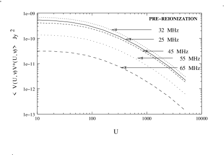
Figure 4: This shows how the visibility correlation $\langle V({\bf U},\nu)V^{*}({\bf U},\nu)\rangle$ varies with baseline $U$. The results are shown for the different frequencies shown in the figure.

The signal strength at any fixed frequency does not vary with $U$ in the range of baselines $10$ to $100$, after which it falls rapidly, falling by an order of magnitude by $U=1000$. Also, with varying frequency the signal falls off quite fast beyond $\sim 45\,{\rm MHz}$. Frequencies smaller than $25\,{\rm MHz}$ will be severely affected by the ionosphere and have not been shown. The visibility correlations as a function $U$ have a very similar behaviour at all the frequencies, with just the amplitude of the signal changing with frequency. The shape of these curves directly reflect the power spectrum at the relevant Fourier modes.

The visibility correlation $\langle V({\bf U},\nu)V^{*}({\bf U},\nu+\Delta\nu)$ for the same baseline and different frequency is shown for $32\,{\rm MHz}$ in Figure 5. The behaviour is similar at other frequencies. The correlation falls rapidly as $\Delta\nu$ is increased. The value of $\Delta\nu$ where the visibilities become uncorrelated scales as $\sim r_{\nu}/(r_{\nu}^{{}^{\prime}}U)$ and it is around $0.8\,{\rm MHz}$ for $U=100$.

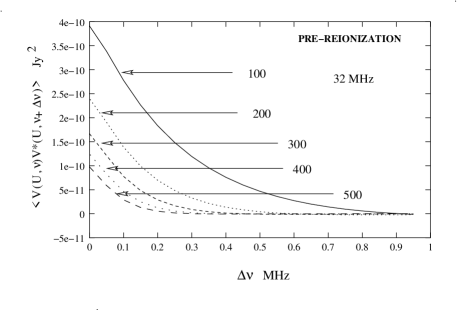
Figure 5: This shows the correlation between the visibilities $V(U,\nu)$ and $V(U,\nu+\Delta\nu)$ expected for the same baseline $U$ at two slightly different frequencies. The result are shown for different values of $U$ (shown in the figure) for the $32{\rm MHz}$ band.

4.2 Reionization

The HI signal here is in emission. The results for the visibility correlation $\langle V({\bf U},\nu)V^{*}({\bf U},\nu)\rangle$ are shown as a function of $U$ for different frequencies in Figure 6. At $\nu\leq 110\,{\rm MHz}$ the hydrogen is largely neutral, and the visibility correlations trace the dark matter power spectrum. The ionization picks up at $\nu=120\,{\rm MHz}$ (Figure 2) where ionized bubbles fill up $\sim 20\%$ of the universe. The centers of these bubbles are clustered with a bias $b_{c}=1.5$ with respect to the underlying dark matter distribution. The presence of these clustered bubbles reduces the signal at small baselines $U\leq 400$. At $130\,{\rm MHz}$ around $50\%$ of the universe is occupied by ionized bubbles. Here the clustering of the bubbles or of the underlying dark matter is of no consequence, and the visibility correlations are due to the discrete nature (Poisson distribution) of the ionized bubbles. The visibility correlation falls drastically for the large baselines which resolve out the bubbles, and the signal at $U>1000$ is due to the clustering of the HI which follows the dark matter. The model for the reionization breaks down when a large fraction of the universe is ionized, and we do not present results beyond $130\,{\rm MHz}$.

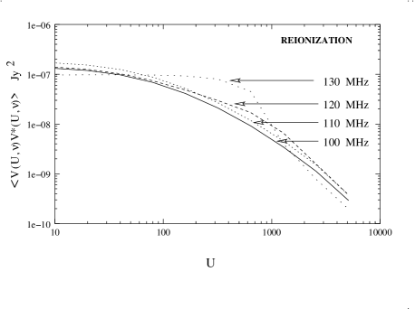
Figure 6: This shows how the visibility correlation $\langle V({\bf U},\nu)V^{*}({\bf U},\nu)\rangle$ varies with baseline $U$. The results are shown for the different frequencies shown in the figure.

An interesting feature when the visibility correlation is dominated by the contribution from individual bubbles is that the fall in $\langle V({\bf U},\nu)V^{*}({\bf U},\nu+\Delta\nu)$ with increasing $\Delta\nu$ is decided by the ratio $R/r_{\nu}^{{}^{\prime}}$. This follows from the fact that the power spectrum $P_{{\rm HI}}$ is now proportional to $W^{2}(kR)$ which falls rapidly for $k\gg 1/R$, and the oscillating integral in eq. (2) cancels out when $\Delta\nu>R/r_{\nu}^{{}^{\prime}}$. The value of $\Delta\nu$ where the visibilities become uncorrelated depends only on the size of the bubbles $R$ and does not change with $U$.

It should be noted that studies of the growth of ionized bubbles (eg. Furlanetto, Zaldarriaga & Hernquist 2004) show them to have a range of sizes at any given epoch during reionization. This will possibly weaken some of the effects like the sharp drop in visibility correlations (Figure 6) and the $\Delta\nu$ dependence (Figure 7) calculated here assuming bubbles of a fixed size.

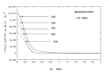
Figure 7: This shows the correlation between the visibilities $V(U,\nu)$ and $V(U,\nu+\Delta\nu)$ expected for the same baseline $U$ at two slightly different frequencies. The result are shown for different values of $U$ (shown in the figure) for the $130{\rm MHz}$ band.

4.3 Post-reionization

The predictions for $\langle V({\bf U},\nu)V^{*}({\bf U},\nu)\rangle$ are shown as a function of $U$ for a variety of frequencies in Figure 8. At all frequencies the correlations are nearly independent of $U$ in the range $10$ to $100$, and then fall by nearly an order of magnitude by $U=1000$. The HI in this era has been assumed to trace the dark matter, and the shape of the curve showing the visibility correlation as a function of $U$ is decided by the dark matter power spectrum at the relevant Fourier modes. The correlations increase with frequency, a reflection of the fact that the matter power spectrum grows with time. It may be noted that the signal also depends on $\Omega_{gas}$ which we have assumed to be a constant over redshift, and the evolution of the signal probes both the growth of the power spectrum and the evolution of $\Omega{gas}$. At a fixed baseline, the correlation $\langle V({\bf U},\nu)V^{*}({\bf U},\nu+\Delta\nu)\rangle$ falls with increasing $\Delta\nu$. The value of $\Delta\nu$ where the visibilities become uncorrelated scales as $\Delta\nu\sim r_{\nu}/r_{\nu}^{{}^{\prime}}U$. The predictions for $\nu=500\,{\rm MHz}$ are shown in Figure 9 where the visibility at $U=100$ becomes uncorrelated at $\Delta\nu\sim 1.3\,{\rm MHz}$. The behaviour is similar at the at the other frequencies.

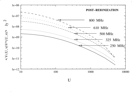
Figure 8: This shows how the visibility correlation $\langle V({\bf U},\nu)V^{*}({\bf U},\nu)\rangle$ varies with baseline $U$. The results are shown for the different frequencies shown in the figure.

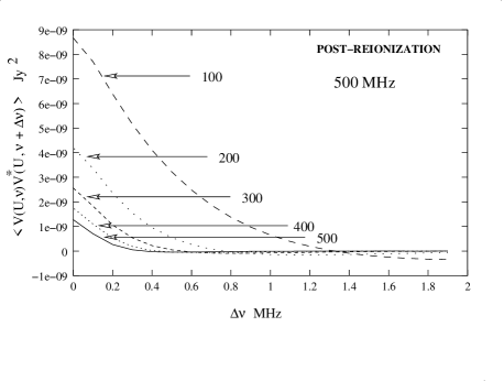
Figure 9: This shows the correlation between the visibilities $V(U,\nu)$ and $V(U,\nu+\Delta\nu)$ expected for the same baseline $U$ at two slightly different frequencies. The result are shown for different values of $U$ (shown in the figure) for the $500{\rm MHz}$ band.

5 Summary and Discussion.

We have proposed that correlations between the visibilities measured at different baselines and frequencies in radio-interferometric observations be used to quantify and interpret the redshifted 21 cm radiation from cosmological HI. This statistics has an inherent advantage over other quantities which have been proposed for the same purpose in that it deals directly with visibilities which are the primary quantities measured in radio-interferometric observations. There is a further advantage in that the system noise in the visibilities measured at different baselines and frequencies is uncorrelated.

The visibility correlations, we show, have a very simple relation to the power spectrum (equation 2), the latter being the statistical quantity most commonly used to quantify the cosmological matter distribution. Also, there is a direct relation between the dimensionless baseline $U$ and the Fourier mode probed by the visibilities at that particular baseline.

We have made predictions for the signal expected over the entire evolution of the HI starting from the dark ages to the present epoch. The magnitude of the signal depends on $\theta_{0}\approx 0.6\times\theta_{FWHM}$ the size of the beam of the individual antenna elements in the array. Our predictions are for $\theta_{0}=1^{\circ}$ at $325{\rm MHz}$ which is appropriate for the GMRT. At other frequencies we have used $\theta_{0}\propto\lambda$ in making our predictions. The results presented here can be easily used to make predictions for other telescopes using the fact that the visibility correlations scale as $\theta_{0}^{2}$. The shape of the curves showing $\langle V({\bf U},\nu)V^{*}({\bf U},\nu+\Delta\nu)\rangle$ as functions of $U$ or $\Delta\nu$ have no dependence on $\theta_{0}$ or any other parameter of the individual antennas. Finally, a reminder that our analysis assumes $\theta_{0}\ll 1$ where the curvature of the sky may be neglected. The analysis will be more complicated for an array of small antennas where the individual elements have a very wide beam, but possibly the qualitative features of this analysis will hold.

One of the salient features of our analysis is that for all the eras the visibility correlation signal from redshifted HI is maximum at small baselines. In the situation where the signal arises mainly from the large scale clustering of the HI whose distribution follows the dark matter the signal is nearly constant up to $U\sim 100$ after which the signal falls rapidly dropping by an order of magnitude by $U\sim 1000$. In the situation when the process of reionization is underway and the HI distribution is patchy, the behaviour of the visibility correlation is decided by the size of the ionized regions. In our model for reionization where there are spherical ionized bubbles of comoving radius $R=3\,h^{-1}{\rm Mpc}$, the visibility correlation is a constant to $U\sim 400$, the larger baselines are not sensitive to the ionized spheres. Details of the reionization model aside, the baseline dependence of the visibility correlations is sensitive to size of the ionized patches and it should be possible to extract this information. Also, an optimal observational strategy would preferentially sample the small baselines where the signal is largest.

We next shift our attention to the correlation between the visibilities at the same baseline but at two different frequencies with separation $\Delta\nu$. We see that the correlations fall off very fast as $\Delta\nu$ is increased. In the situation where the visibility correlation signal is from the large scale gravitational clustering of the HI the value of $\Delta\nu$ where the visibilities become uncorrelated scales as $r_{\nu}/(r_{\nu}^{{}^{\prime}}U)$ and it is around $1\,{\rm MHz}$ at $U=100$ at all frequencies. In the situation where the signal is from ionized patches, the value of $\Delta\nu$ where the visibilities become uncorrelated is decided by $R/r_{\nu}^{{}^{\prime}}$ and it is around $0.4\,{\rm MHz}$ independent of the value of $U$. This feature should allow us to determine from the observations whether it is the large scale gravitational clustering of the HI or the ionized patches which dominates the visibility correlation. The latter is expected to dominate during the epoch when reionization is underway. It may be noted that the value $0.4\,{\rm MHz}$ quoted here is specific to the model of reionization which we have adopted. Though the value is model dependent, we expect that the qualitative features discussed here should continue to hold even in a more general situation.

The main challenge in observing cosmological HI is to extract the HI signal from the various contaminants which are expected to swamp this signal. The contaminants include Galactic synchrotron emission, free-free emission from ionizing halos (Oh & Mack, 2003), faint radio loud quasars (DiMatteo. et al., 2002) and synchrotron emission from low redshift galaxy clusters (DiMatteo. et al., 2004). Fortunately, all of these foregrounds have smooth continuum spectra whose contribution varies slowly with frequency. The contribution from these contaminants to the visibilities at the same baseline but two frequencies differing by $\Delta\nu$ will remain correlated for large values of $\Delta\nu$, whereas the contribution from the HI signal will be uncorrelated beyond something like $1\,{\rm MHz}$ or even less depending on the value of $U$. It is, in principle, straightforward to fit the visibility correlation at large $\Delta\nu$ and remove any slowly varying component thereby separating the contaminants from the HI signal.

Finally, we briefly discuss the level of visibility correlation detectable in a radio-interferometric observation. We consider an array of $N$ antennas, the observations lasting a time duration $t$, with frequency channels of width $\delta\nu$ spanning a total bandwidth $B$. It should be noted that the effect of a finite channel width $\delta\nu$ has not been included in our calculation which assumes infinite frequency resolution. This effect can be easily included by convolving our results for the visibility correlation with the frequency response function of a single channel. Preferably, $\delta\nu$ should be much smaller than the frequency separation at which the visibility correlation become uncorrelated. We use $S$ to denote the frequency separation within which the visibilities are correlated, and beyond which they become uncorrelated. The rms. noise in the a single visibility correlation is (Thompson, Moran & Swenson, 1986)

$$\sqrt{\langle(VV*)^{2}\rangle}=\left(\frac{2k_{B}T_{SYS}}{A_{ef}}\right)^{2}\frac{1}{\delta\nu\,t}$$ (24)

where $T_{SYS}$ is the system temperature and $A_{ef}$ is the effective area of a single antenna. The noise contribution will be reduced by a factor $1/\sqrt{N_{o}}$ if we combine $N_{o}$ independent samples of the visibility correlation. A possible observational strategy for a preliminary detection of the HI signal would be to combine the visibility correlations at all baselines and frequency separations where there is a reasonable amount of signal. This gives $N_{o}=[N(N-1)/2]\,(B/\delta\nu)\,(S/\delta\nu)$ whereby

$$\sqrt{\langle(VV*)^{2}\rangle}=\left(\frac{2k_{B}T_{SYS}}{A_{ef}}\right)^{2}\,\frac{1}{t}\,\sqrt{\frac{2}{N(N-1)\,B\,S}}\,.$$ (25)

Using values for the GMRT (at $\sim 325\,{\rm MHz}$), $(2k_{B}T_{SYS}/A_{ef})=144\,{\rm Jy}$, $B=16\,{\rm MHz}$, there are $14$ antennas within $U\leq 1000$ where the signal is strong and $S=0.5\,{\rm MHz}$ beyond which the signal is uncorrelated we find that it is possible to achieve noise levels of $\sqrt{\langle(VV*)^{2}\rangle}=1.0\times 10^{-9}\,{\rm Jy}^{2}$ which is below the signal with $200\,{\rm hrs}$ of integration.

We shall investigate in detail issues related to detecting the HI signal, the necessary integration time for different telescopes and signal extraction in a forthcoming paper.

Appendix A The optical depth of the redshifted HI 21 cm line.

The optical depth is defined as

$$\tau_{\nu}(l)=\int^{l}_{l0}\alpha_{\nu}(l^{\prime})dl^{\prime}$$ (26)

where $\alpha_{\nu}$ is the absorption coefficient for the redshifted 21 cm line given by

$$\alpha_{\nu}=\frac{h_{P}\nu_{e}}{4\pi}\phi(\nu)[n_{0}B_{01}-n_{1}B_{10}]\,.$$ (27)

Here $\phi(\nu)$ is the line profile function, and $B_{01}$ and $B_{10}$ are the Einstein coefficients (Rybicki. & Lightman, 1979) for the 21 cm line. We use $r(\nu)$ to denote the comoving distance from which the $1420\,{\rm MHz}$ radiation will be redshifted to the frequency $\nu$ for an observer at present. The HI radiation from a physical line element $\Delta l$ at the epoch when the HI radiation originated will be spread over a frequency range $\Delta\nu=(\partial r(\nu)/\partial\nu)^{-1}\,(\Delta l/a)$ at the observer. Here $a=1/(1+z)$ is the scale factor. The line profile function $\phi(\nu)$, defined at the epoch when the HI radiation originated, is a step function of width $a/\Delta\nu$. It then follows that

$$\int\phi(\nu)\,dl=a^{2}\frac{\partial r(\nu)}{\partial\nu}$$ (28)

and the optical depth can be written as

$$\tau_{\nu}=\frac{h_{P}\nu_{e}}{4\pi}n_{0}B_{01}(1-\frac{g_{0}}{g_{1}}\frac{n_{0}}{n_{1}})a^{2}\mid\frac{\partial r(\nu)}{\partial\nu}\mid\,.$$ (29)

The Einstein coefficients are related by $B_{01}=3B_{10}=\frac{3\lambda_{e}^{3}}{2h_{p}c}A_{10}$ , where $A_{10}=2.85\times 10^{-}{15}$ $s^{-1}$ is the spontaneous emission coefficient of the 21 cm line . So the optical depth finally becomes

$$\tau_{\nu}=\frac{3n_{HI}h_{p}c^{2}A_{10}a^{2}}{32\pi k_{B}T_{s}\nu_{e}}\mid\frac{\partial r(\nu)}{\partial\nu}\mid$$ (30)

where $n_{HI}$ is the number density of HI atoms. In presence of peculiar velocity $r(\nu)$ is given by

$$r(\nu)=\int^{1}_{\frac{\nu}{\nu_{e}(1-v/c)}}\hskip 5.69046pt\frac{c\,da}{a^{2}\,H(a)}$$ (31)

where $v$ is the line of sight component of the peculiar velocity of the HI. This gives us

$$\mid\frac{\partial r(\nu)}{\partial\nu}\mid=\frac{\lambda_{e}}{a^{2}H(z)}[1-\frac{1}{aH(z)}\frac{\partial v}{\partial r_{\nu}}]$$ (32)

where $r_{\nu}$ is the same as $r(\nu)$ without the effect of peculiar velocities, and where we have retained only the most dominant term in the peculiar velocity. Using this it is possible to write the optical depth as

$$\tau_{\nu} = \frac{4.0\,\rm mK}{T_{s}}\,\left(\frac{\Omega_{b}h^{2}}{0.02}\right)\left(\frac{0.7}{h}\right)\frac{H_{0}}{H(z)}(1+z)^{3}\,$$ (33)

$$\times \frac{\rho_{{\rm HI}}}{\bar{\rho}_{{\rm H}}}\,\left[1-\frac{(1+z)}{H(z)}\frac{\partial v}{\partial r_{\nu}}\right]$$

where $\rho_{{\rm HI}}/\bar{\rho}_{{\rm H}}$ is the ratio of the neutral hydrogen to the mean hydrogen density.

References

- Bagla, Nath and Padmanabhan (1997) Bagla J.S., Nath B. and Padmanabhan T. 1997, MNRAS 289, 671
- Bagla & White (2002) Bagla J.S. and White M. 2002, astro-ph/0212228
- Barkana & Loeb (2001) Barkana R. & Loeb A.,2001,Phys.Rep.,349,125
- Becker et al. (2001) Becker,R.H.,et al.,2001,AJ,122,2850
- Bharadwaj, Nath & Sethi (2001) Bharadwaj S., Nath B. & Sethi S.K. 2001, JApA.22,21
- Bharadwaj & Sethi (2001) Bharadwaj, S. & Sethi, S. K. 2001, JApA, 22, 293
- Bharadwaj & Pandey (2003) Bharadwaj, S. & Pandey, S. K. 2003, JApA, 24, 23
- Bharadwaj & Srikant (2004) Bharadwaj, S. & Srikant p,s. 2004, JApA, in press
- Bharadwaj & Ali (2004) Bharadwaj S. & Ali S. S. 2004, MNRAS,in Press,
- Chen & Miralda-Escude (2004) Chen, X. & Miralda-Escude,J.,2004, Ap.J, 602, 1
- Ciardi & Madau (2003) Ciardi,B.& Madau,P. 2003,Ap.J,596,1
- DiMatteo. et al. (2004) DiMatteo,T.,Ciardi,B.,Miniati,F.2004,MNRAS,submitted,astro-ph/0402332
- DiMatteo. et al. (2002) DiMatteo,T.,Perna R.,Abel,T.,Rees,M.J.2002,Ap.J,564,576
- Fan et al. (2002) Fan,X.,et al. 2002,AJ,123,1247
- Furlanetto,Sokasian. & Hernquist (2003) Furlanetto, S. R.,Sokasian A. & Hcernquist L.2003,astro-ph/0305065
- Furlanetto, Zaldarriaga & Hernquist (2004) Furlanetto, S. R., Zaldarriaga, M. & Hcernquist L. 2004, astro-ph/0403697
- Gnedin & Ostriker (1997) Gnedin, N. Y. & Ostriker, J. P,1997,Ap.J,486,581
- Gnedin & Shaver (2003) Gnedin, N. Y. & Shaver, P. A.2003,astro-ph/0312005
- Gruzinov & Hu (1998) Gruzinov, A. & Hu, W. 1998,Ap.J,508,435
- Hogan & Rees (1979) Hogan, C. J. & Rees, M. J., 1979, MNRAS,188,791
- Hui & Haiman (2003) Hui, L., & Haiman, Z., 2003, ApJ,596,9
- Iliev et al. (2002) Iliev,I.T.,Shapiro,P.R.,Farrara,A.,Martel,H.2002,Ap.J,572,L123
- Iliev et al. (2003) Iliev,I.T.,Scannapieco,E.,Martel,H.,Shapiro,P.R. 2003,MNRAS,341,81
- Kaiser (1987) Kaiser N. 1987, MNRAS,227,1
- Kumar, Padmanabhan & Subramanian (1985) Kumar A., Padmanabhan T. and Subramanian K., 1995, MNRAS, 272, 544
- Knox at al. (1998) Knox L.,Scoccimarro R. & Dodelson S.1998,Physical Review Letters,81,2004
- Lahav et al. (1991) Lahav, O., Lipje, P. B., Primack, J. R. and Rees, M. J. 1991, MNRAS,251, 128
- Lanzetta, Wolfe & Turnshek (1998) Lanzetta, K. M., Wolfe, A. M., Turnshek, D. A. 1995, ApJ, 430, 435
- Loeb & Zaldarriaga (2003) Loeb A. & Zaldarriaga, M.,2003,astro-ph/0312134
- Madau, Meiksin & Rees (1997) Madau P., Meiksin A. & Rees, M. J.,1997,Ap.J,475,429
- Miralda-Escude (2003) Miralda-Escude,J.,2003,Science 300,1904-1909
- Morales (2004) Morales, M. F. 2004, preprint, astro-ph/0406662
- Morales & Hewitt (2003) Morales, M. F. and Hewitt, J., 2003, ApJ, Submitted (astro-ph/0312437)
- Oh & Mack (2003) Oh,S.P.,& Mack,K.J.,2003,MNRAS,346,871
- Péroux et al. (2001) Péroux, C., McMahon, R. G., Storrie-Lombardi, L. J. & Irwin, M .J. 2003, MNRAS, 346, 1103
- Rybicki. & Lightman (1979) Rybicki, G. B. & Lightman, A. P.,1979,Radiative Processes in Astrophysics.Willey,New York,pp. 29-32
- Santos, Cooray & Knox (2004) Santos, M.G., Cooray, A. & Knox, L. 2004, preprint, astro-ph/0408515
- Saini, Bharadwaj & Sethi (2001) Saini T., Bharadwaj S. & Sethi, K. S. 2001, ApJ, 557, 421
- Scott & Rees (1990) Scott D. & Rees, M. J., 1990, MNRAS,247,510
- Shaver et al. (1999) Shaver, P. A., Windhorst, R, A., Madau, P.& de Bruyn, A. G.,1999,Astron. & Astrophys.,345,380
- Spergel et al. (2003) Spergel, D. N.,et al. 2003,ApJS,148,175
- Subramanian & Padmanabhan (1993) Subramanian K. and Padmanabhan T., 1993, MNRAS, 265, 101
- Sunyaev and Zeldovich (1972) Sunyaev, R. A. & Zeldovich, Ya. B., 1972,Astron. & Astrophys,22,189
- (44) Storrie–Lombardi, L. J., McMahon, R. G., Irwin, M. J. 1996, MNRAS, 283, L79
- Tegmark et al. (2003a) Tegmark, M., et al., 2003a, Ap.J, Submitted (astro-ph/0310725)
- Tegmark et al. (2003b) Tegmark, M., et al., 2003b, Ap.J, Submitted (astro-ph/0310723)
- Theuns et al. (2002) Theuns, T. et al., 2002, ApJ,567,L103
- Thompson, Moran & Swenson (1986) Thompson, A.R., Moran, J.M. and Swenson, G.W., Jr. 1986, Interferometry and Synthesis in Radio Astronomy, John Wiley and Sons, New York, pp 162-165
- Tozzi et al. (2000) Tozzi.P.,Madau.P.,Meiksin. A.,Rees,M.J.,2000,Ap.J,528,597