The Cooling Behavior of Thermal Pulses in Gamma-Ray Bursts

Abstract

We discuss gamma-ray bursts (GRBs) that have very hard spectra, consistent with black-body radiation. Several emission components are expected, on the basis of theoretical considerations, to be visible in the gamma-ray band, mainly non-thermal emission from cooling, relativistic electrons and thermal emission from a wind photosphere. We find that the pulses we study are consistent with a thermal, black-body radiation throughout their duration and that the temperature, $kT$, can be well described by a broken power-law as a function of time, with an initially constant or weak decay ($\sim 100$ keV). After the break, most cases are consistent with a decay with index $-2/3$. A few of the pulses have a weak non-thermal component overlayed the thermal one, and are better fitted with a combination of a thermal and a non-thermal component. We further demonstrate that such a two-component model can explain the whole time-evolution of other bursts, that are found to be only initially thermal and later become non-thermal. The relative strengths between the two components vary with time and this is suggested to, among other things, account for the change in the modelled low-energy power-law slope that is often observed in GRBs. The secondary, non-thermal components are consistent with optically-thin synchrotron emission in the cooling regime. We interpret the observations within a model of an optically thick shell (fireball) that expands adiabatically. The slow, or constant, temperature decrease is from the acceleration phase, during which the bulk Lorentz factor increases, and the faster temperature decay is reached as the flow saturates and starts to coast with a constant speed. We also discuss a Poynting-flux model, in which the saturation radius is reached close to the photosphere. Even though these observations cannot tell these models apart, the latter has several attractive advantages. The GLAST satellite will be able to clarify and further test the physical setting of similar thermal pulses.

1 Introduction

The radiation from gamma-ray bursts (GRBs) is assumed to arise in a highly relativistic outflow from a collapsing massive progenitor star. This outflow could either be in a form of a strongly magnetized wind, where most of the energy is transported in magnetic fields, or in a low-baryon-load ’fireball’ where the energy is transported mainly as kinetic energy. In both cases the outflow is initially optically thick and will emit thermal radiation. As the flow expands the typical photon energy and the number density will decrease. At a certain distance from the progenitor it will become optically-thin to pair production and Compton scattering off the free electrons associated with the baryons in the outflow, and the radiation decouples from the matter and escapes to an observer at infinity. The plasma then emits a strong flash of thermal black-body radiation. Beneath this photosphere the radiation created by the dissipation of energy is transformed back into the kinetic energy of the flow. As the outflow becomes transparent, non-thermal radiation processes such as synchrotron and/or inverse Compton processes can radiate away the dissipated energy, by transforming it into the gamma-rays. In the fireball model, the wind has a variable initial distribution of Lorentz factors, often thought of as individual shells moving with various speeds. In this outflow shocks are created, at a typical distance of $\sim 10^{14}$ cm from the center of the progenitor, which dissipate the energy and accelerate the electrons which cool and radiate. The radiation could also stem from shocks created as the wind interacts with the external medium surrounding the progenitor. On the other hand, in the magnetic-energy dominated, or Poynting flux models, the magnetic field energy is assumed to be dissipated locally through reconnections, and is then transformed into $\gamma$-rays by the accelerated electrons.

The observed spectrum from a GRB is therefore expected to be a superposition of the thermal black-body and the synchrotron/inverse Compton emissions generated in the optically-thin environments. Depending on the initial conditions of the outflow, the radiative efficiencies in the shocks and/or reconnection rates, these components will be of different importance (Mészáros et al., 2002; Drenkhahn & Spruit, 2002). For instance, Daigne & Mochkovitch (2002) calculated the expected photospheric black-body luminosity and temperature for various fireball models. For the standard model they found that the internal energy will still be large at typical photosphere radii, and thus the thermal component of the spectrum will be very hot and luminous. Depending on the observed energy band it could even be dominating the spectrum, even when the radiative efficiency in the shocks is very high. Similarly, Drenkhahn & Spruit (2002) found in numerically modelling of strongly magnetized winds from GRBs that, for certain initial conditions, the amount of energy emitted as thermal radiation can indeed be large.

Most observed GRB light curves are dominated by a non-thermal radiation (Preece et al., 2000) and a large fraction of these are consistent with various versions of an optically-thin, intrinsic synchrotron spectrum, that is, consistent with a photon index of $\alpha<-2/3$ (see eq. [1] below for the definition of $\alpha$). This radiation naturally stems from energy dissipation in optically-thin regions and is usually interpreted as the signature of, for instance, the internal shocks. Furthermore, the power-law below the peak energy, i.e. $\alpha$, is variable for more than half of all bursts, and of these, it softens in general (Crider et al., 1997). However, a notable fraction of the time-resolved spectra are harder than optically-thin synchrotron spectra, that is, inconsistent with $\alpha<-2/3$, the so-called line-of-death for the synchrotron model (Preece et al., 1998). It is mainly spectra early on in the pulse light-curve that are the hardest. Aside from theoretical motivations mentioned above [see, e.g., Mészáros et al. (2002); Daigne & Mochkovitch (2002); Drenkhahn & Spruit (2002); Blinnikov et al. (1999)], several authors have already proposed a thermal origin as an interpretation of the very hardest observed time-resolved spectra at early times, for instance Crider et al. (1997); Ghirlanda et al. (2003a). However, no conclusive picture has yet emerged explaining these ’hard’ spectra and especially their spectral evolution. In this paper, we identify a few bursts which are consistent with black body emission throughout the burst, which has not been reported before. These are presented in §2 and their behavior is analyzed in §3. We interpret these as bursts in which the initial conditions are such that the thermal photospheric emission component dominates over the optically-thin emission from the dissipated free energy. We can thus study the temperature behavior by modelling the spectrum with an intrinsic black-body spectrum. We also analyze a few pulses in which a power-law component in the spectrum becomes more and more dominant, thus accounting for the initially hard bursts and their spectral evolution. We discuss this interpretation in §4 and we conclude our discussion in §5.

2 The Sample of Thermal Pulses and the Analysis Method

To find bursts that are dominated by a thermal emission, we search among bursts that have a prominent, single pulse(s). The motivations for this is manyfold. First, the hardest spectra that have been reported are time-resolved spectra at the beginning of simple pulse structures (see, e.g., Ghirlanda et al. (2003a)). Second, in the numerical study of single-pulsed GRBs within the standard internal shock model, Daigne & Mochkovitch (2002) concluded that the thermal component should be in most cases at least as bright as the non-thermal component for such pulses. Third, in several other theoretical/numerical modelings (e.g., Ruffini et al. (2001) and Lyutikov & Usov (2000)) a single, thermal, precursor-pulse (’proper-GRB’ in Ruffini et al. (2001)) is found to preceed the more variable main burst emission. Fourth, from a theoretical point of view the variability of a burst is closely related to the location of the photosphere (e.g., Kobayashi, Ryde, & MacFadyen (2002)). The further out the photosphere is, for instance due to low bulk Lorentz factors, the less efficient are the internal shocks and the less variable are the light curves. In these cases the thermal photosphere could be expected to be relatively stronger. Fifth, in the analysis in McQuinn, Ryde, & Petrosian (2004, in prep.) we conclude that the curvature effect is more prominent for hard spectral bursts, such we here interpret as thermal, compared to non-thermal bursts. This effect is due to differences in light-travel times, and Lorentz boosts for photon emitted from a curved surface. It has a strong effect on the light curves, making them smoother. All these arguments point to that pure thermal emission is expected to be a smooth pulse, or at least dominated by one, while the non-thermal emission from the internal shocks and/or reconnections is expected to be highly variable with complicated light curves. This therefore motivated us to search for photospheric bursts in the catalogue of GRB pulses by F. Ryde et al. (in prep.). These bursts are a subsample of the CGRO BATSE catalogue and comprise strong, single pulses. The selection criterion that was used for these pulses required the peak flux to be greater than 1.0 photons cm^-2 s^-1 on a 256 ms timescale. Of these, bursts were selected that exhibited clean, single-peaked events, or in the case of multi-peaked bursts, pulses that were well separated and distinguishable from each other. The catalogue is limited to pulses with durations longer than 2 s (full width–half max). In the search we did not assume any functional description of the pulse profile in order to eliminate any preconceived idea of what the fundamental pulse shape should be. The final sample consisted of 76 pulses within 68 bursts. This sample has also been used in other connections, for instance, in Kocevski, Ryde, & Liang (2003).

The data were gathered by BATSE’s Large Area Detectors (LADs), which flew on the Compton Gamma-Ray Observatory (CGRO). We used mainly the high-energy resolution burst (HERB) data (Fishman et al., 1989). The HERB data have 128 energy channels covering approximately 10 keV to several MeV, with sub-second time-resolution. A background estimate was made using the HER data, which consist of low (16–500 s) time resolution measurements that are stored between triggers. The light curve of the background, during the outburst, was modelled by interpolating these data, roughly 1000 s before and after the trigger, with a second or third order polynomial fit. The data, as well as the background fit coefficients were obtained from the CGRO Science Support Center (GROSSC) at Goddard Space Flight Center through its public archives. The central part of the analysis was performed with the RMFIT package, version 1.0b1 (Malozzi et al. 2000) and the spectral fitting was done using the MFIT package, version 4.6, running under RMFIT. We always chose the data taken with the detector which was closest to the line-of-sight to the location of the GRB, as it has the strongest signal. The broadest energy band with useful data was selected, which is often approximately 25–1900 keV, as the lowest $\sim$ 8 channels of the HERB data are usually not useful. Although BATSE’s spectroscopic detectors (SDs) can gather enough data to produce spectra on a 0.128 s timescale, the data usually have to be integrated to get an acceptable fit to a given spectra model. This reduces the resolution of the time-history significantly. The background-subtracted photon spectrum, $N_{\rm E}(E)$, was determined using a forward-folding technique. A spectral model was folded through the detector response matrix and was then fitted by minimizing the $\chi^{2}$ (using the Levenberg-Marquardt algorithm) between the model count spectrum and the observed count spectrum, giving the best-fit spectral parameters and the normalization.

In our search for photospheric candidates, we fitted the spectra using a Planck function described by equation (3) below. The bursts that were found to be reasonably well fitted by black bodies were selected: GRB930214 (BATSE trigger #2193), GRB941023 (#3256), GRB951228 (#4157), GRB971127 (#6504), GRB990102 (#7295). These are presented in Table 1, where they are denoted by both their GRB names and BATSE trigger numbers. We also present, in Figure 1, the 64 ms resolution count light-curves. These data have the maximal time-resolution, but have only four energy channels. The peak times are also given in the table.

To characterize the time-integrated spectra of the pulses, we model them with the empirical function (the ’GRB-function’; Band et al. (1993)):

$$N_{\rm E}(E)=\left\{\begin{array}[]{ll}C\ E^{\alpha}e^{-E/E_{\rm 0}}&\mbox{if $(\alpha-\beta)E_{\rm 0}\geq E$}\\ C^{\prime}E^{\beta}&\mbox{if $(\alpha-\beta)E_{\rm 0}<E$ ,}\end{array}\right.$$ (1)

where $E$ is the energy in keV, $E_{\rm 0}$ is the $e-$folding energy, $\alpha$ and $\beta$ are the asymptotic power law indices, $C$ the amplitude, and $C^{\prime}$ has been chosen to make the photon spectrum, $N_{\rm E}(E)$, a continuous and a continuously differentiable function through the condition

$$C^{\prime}=C\left[(\alpha-\beta)E_{\rm 0}\right]^{\alpha-\beta}e^{-(\alpha-\beta)}.$$ (2)

The peak energy, $E_{\rm pk}$, at which the $EF_{\rm E}$-spectrum ($F_{\rm E}\equiv EN_{\rm E}$) is at its maximum, is used as a measure of the spectral hardness instead of $E_{\rm 0}$. They are related by $E_{\rm pk}=(2+\alpha)E_{\rm 0}$. The properties of the time-integrated spectra are given in table 2. In particular, we want to draw attention to the low-energy power-law indices, $\alpha$, which, in general, are hard, that is, larger than $-2/3$, but they are all lower than, for instance $+1$, the Rayleigh-Jeans spectrum of a black body (see §3). One case, trigger 3256, even has a slope that is softer than $-2/3$, even though the time-resolved spectra are hard. The instantaneous and the time-integrated spectra are, in general, different, since there is significant spectral evolution.

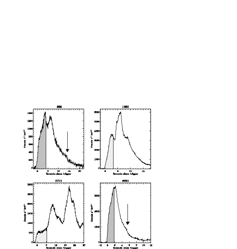
Figure 2: During the initial phase of these bursts, marked by the shaded areas, the spectra are consistent with a black body spectrum. The arrows draw attention to the breaks in the light curve. See the text for details.

We will later also discuss other bursts that have previously been found to have hard spectra, consistent with black bodies, but only in the initial phase of the burst. These quickly become non-thermal: 910927 (#829), 911118 (#1085), GRB 970111 (#5773) and GRB980306 (#6630). These pulses are shown in Figure 2.

3 Spectral Modelling

3.1 Thermal and non-thermal spectra

The time-resolved, thermal spectra of the pulses, identified in the previous section, are modelled by a Planck function, which is the characteristic spectrum from an optically-thick medium in which the mean-free-path of a photon is short and the radiation is completely coupled to the matter. The background-subtracted photon spectrum, $N_{\rm E}(E,t)$, for each time bin of the observations, is thus modelled by (Planck, 1901)

$$N_{\rm E}(E,t)=A(t)\,\,\frac{E^{2}}{exp[E/kT(t)]-1}=A\,(kT)^{2}\,\frac{x^{2}}{(e^{x}-1)},$$ (3)

where $x\equiv E/kT$ and $kT$ is the color temperature of the black-body in keV, and $k$ is the Boltzmann constant ($8.617\times 10^{-8}$ keV/K). The fitted parameters are thus the normalization $A$ and temperature $kT$, and the quality of the fit is given by a reduced $\chi^{2}$-value ($\equiv\chi^{2}_{\nu}$). For small photon energies compared to the temperature ($E<<kT$) the Planck function approaches the Rayleigh-Jeans Law $N_{\rm E}(E)\propto E$, and at large energies ($E>>kT$) it approaches the Wien law $N_{\rm E}(E)\propto E^{2}\exp(-E/kT)$. In the discussion below we will denote the spectrum below $kT$ as the Rayleigh-Jeans portion of the spectrum and similarly, the Wien portion of the spectrum is that above $kT$. Strictly speaking, however, the asymptotic laws are not reached until several decades away from $kT$. This is illustrated in figure 3, in which a Planck curve (solid line) is shown in a $EF_{E}$-representation. The energy interval 20 keV – 2 MeV is also indicated. It is clear from the figure that the Rayleigh-Jeans power-law is barely reached within the first decade below the peak. This aspect is important to bear in mind when observations in a finite band is interpreted.

Non-thermal GRB spectra are often interpreted as being the result of synchrotron emission from a distribution of relativistic electrons. In the simplest version of the model the radiation is emitted from an optically-thin plasma in which the electron pitch-angles are isotropically distributed (Pacholczyk, 1970). In relativistic shocks, electrons are accelerated, through various mechanisms, into a power-law distribution in Lorentz factors, say with index $p$ and within an interval of Lorentz factors [$\gamma_{\rm min}\leq\gamma\leq\gamma_{\rm max}$]; $f(\gamma)\propto\gamma^{-p}$. If the electrons cool on a very short time-scale, this distribution will steepen by unity; $-(p+1)$. For instance, for the Fermi type of particle acceleration in relativistic shocks $p\sim 2.2$ (Mészáros, 2002). However, the nature of the actual acceleration mechanism that takes place in GRBs is not well understood.

In all cases, the distribution of electrons will give rise to a characteristic photon spectrum with a peak at an energy that is related to the minimum value of the electron Lorentz factors, $E_{\rm p}\propto\gamma_{\rm min}^{2}h\nu_{B}$, where $\nu_{\rm B}=eB_{\perp}/2\pi m_{\rm e}c$ is the gyrofrequency in a magnetic field with a mean perpendicular component $B_{\perp}$. Below this frequency the spectrum approaches a power law with index $\alpha=-2/3$, while at higher energies the power law will have an index of $\beta=-(p+1)/2$ (cooling effects are negligible) or $\beta=-(p+2)/2$ (cooling spectrum). The main contribution to the low-energy spectrum is from the lowest energy electrons emitting with their characteristic spectrum. The value of $\alpha=-2/3$ is therefore the largest (hardest) value that optically-thin synchrotron-emission can yield. To approximately model such spectra various versions of broken power-laws have been used, for instance the GRB-function [eq. (1)]. In §3.3 below we will characterize the non-thermal contribution to the spectrum by a single power-law, which is the best allowed by the data, but nevertheless informative.

3.2 Evolution of the Black-body Spectra

3.2.1 Planck Model Fits

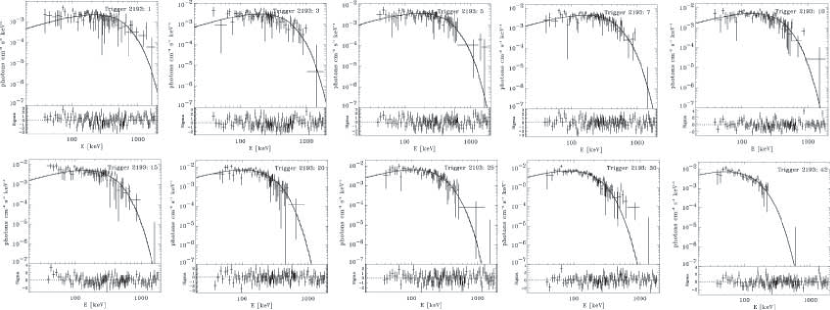
Figure 4: Black-body fits to the time-resolved spectra of burst 2193. The spectra correspond to the following time bins (compare fig. [1]), 1: 1.6 – 2.4 s, 3: 3.14 – 3.84 s, 5: 4.5 – 5.3 s, 7: 6.0 – 6.7 s, 10: 8.0 – 8.7 s, 15: 11.3 – 11.9 s, 20: 14.6 – 15.2 s , 25: 18.0 – 18.8 s, 30: 21.6 – 22.9 s, 42: 39.4 – 41 s.

The results of the spectral modelling of the five triggers in the sample with a black body model is depicted in Figures 4 to 8. Here, the time-resolved photon-flux spectral data are shown, as well as the corresponding best-fit Planck function (eq. [3]). The crosses correspond to the deconvolved data points in photons cm^-2 s^-1 keV ^-1 and the spectra are rebinned to have a SNR=1 to make the plots clearer. Ten characteristic time-bins were selected for each case to illustrate the time evolution of the spectra during the pulses.

The first conclusion that can be drawn from the figures is that a Planck function fits the data well for the portion of the spectrum below $kT$, i.e. at low energies, which is approaching the Rayleigh-Jeans spectrum. Also at the high energies all but triggers 6504 and 7295 fit the data acceptably well. These two triggers have additional high-energy flux compared to the best-fit black-body model and there is clearly need for an additional, weaker spectral component that affects the spectrum at high energies. They will therefore be further studied below. In the figures, the residual patterns for the time-resolved fits, i.e., the differences between the data and the best-fit-model fluxes in units of $\sigma$, are shown below every spectrum. They are small and do not show any strong systematic trends, something that would appear in poor fits. Therefore, we conclude that the five triggers in the sample are consistent with the picture of them being dominated by emission from an optically thick environment, or a photosphere, throughout the evolution during the pulses.

To further illustrate the modelling, the time-resolved values of $\chi_{\nu}^{2}$ are plotted as a function of time for all five cases in Figure 9. These $\chi^{2}_{\nu}$-values are all reasonable and they do not show any strong temporal evolution, disregarding trigger 6630 (which is not one of the thermal pulses), which is indicative of good fits. In addition, the $\chi^{2}_{\nu}$ for the whole pulse is shown in the Figure as the dashed line, for each case. This is the summed $\chi^{2}$-value for all the spectra divided by the total number of degrees of freedom (d.o.f.). They too have reasonable values, which is to be expected as the time resolved fits were good.

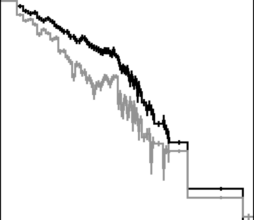
Figure 10: The BATSE raw data (solid black line), in counts s^-1 keV^-1 for the peak of bursts 7295, illustrating the background signal (grey line) compared to the GRB data. The studied interval is marked by the solid, vertical lines and the signal-to-noise ratio, SNR=1.

In interpreting the observed spectra and the fits to them, it should be noted that the low-energy bins (as well as the high energy ones) have a lower significance compared to the bins between, say 50 and 1000 keV, due to the detector sensitivity and the background. The spectra in Figures 4 to 8 were rebinned to increase the clarity. The flux error-bars are placed at an averaged energy of the new, broader energy bin, weighted by the observed flux. This is necessary to correctly reproduce the statistics of the observations, especially for the high-energy bins. To illustrate this further, we plot in Figure 10 the raw detection of the burst 7295. The background count-rate is shown by the gray curve and the total flux is shown by the solid line. The background is subtracted from these raw data to find the burst spectrum, which is then modelled. Especially for the cases studied here, which mainly have spectra that fall off exponentially toward higher energies, the burst signal quickly gets weaker, forcing the high-energy bins to be broad to achieve a higher signal-to-noise ratio. Note, however, that the $\chi^{2}$ fitting of the model is made with the full resolution of the detector, which can be seen in the residual plots below the spectra, in the previous figures.

3.2.2 Is a Planck spectrum a unique interpretation?

This fact, discussed at the end of the previous section, together with the proximity of the peak of the spectrum to the low-energy band-limit of the detector, makes it problematic to prove, beyond any doubt, the thermal character of the spectra. Ideally, one would like to reach the asymptotic photon index $\alpha=+1$ (compare Fig. 3) to demonstrate the black body character conclusively. Several other emission mechanism do produce hard-$\alpha$ spectra. This is the case, for instance, for optically-thin synchrotron radiation with a small pitch-angle distribution ($N_{\rm E}\propto E^{0}$) (Lloyd-Ronning & Petrosian, 2000), or similarly, jitter radiation, where the magnetic fields have a correlation length less than the Larmour radius of the electrons. Also a typical optically-thin synchrotron spectrum ($\propto E^{-2/3}$) can be deformed due to scattering in a hot cloud it traverses and reach $\alpha\sim 0$ for high optical depths (Dermer & Boettcher, 2000). The high-energy portion of the spectrum would be largely unaffected due to the decline in the scattering cross-section with energy. But all these spectra have a high-energy power-law distribution, in contrast to the exponential cut-offs observed above. Hard low-energy spectra, combined with an exponential cut-off, are given, for instance, by saturated Comptonization, with its Wien peak $N_{\rm E}(E)\propto E^{2}exp(-E/kT)$ (see, e.g., Liang (1997)). The low-energy spectra are, however, even harder spectra than the Planck function ($\alpha=+2$). Also the Compton drag model (Ghisellini et al., 2000) produces a hard low-energy spectrum ($\alpha\sim 1$) and a steep high-energy tail. These spectra are, in general, broader than a Planck spectrum and the possibility, within the model, of producing several pulses following immediately after each other is not clear (Ghirlanda et al., 2003a). Furthermore, inverse Compton scattering of soft, synchrotron, seed photons, by the emitting electrons themselves (synchrotron self-Compton), will have a spectrum that has $\alpha=0$ at low-energy, if the electron distribution is near to mono-energetic and the seed photons have a self-absorbed spectrum (Rybicki & Lightman (1979)). A physical scenario for this to arise is discussed in detail by Stern & Poutanen (2004). These spectra are however somewhat broad and require high peak-energies for the $\alpha=0$ power-law to be noticeable in the BATSE band. A broader electron distribution and/or seed photon spectrum will also, by necessity, make the spectrum softer. Yet another possibility, for such a hard spectrum, is optically-thin thermal synchrotron emission. The spectra are approximately described by (Petrosian, 1981; Wardziński & Zdziarski, 2000)

$$N_{\rm E}(E)\propto\exp\left[-\left(\frac{4.5}{\sin\vartheta}\frac{\nu}{\nu_{c}\Theta^{2}}\right)^{1/3}\right]$$ (4)

where $\nu_{c}=eB/2\pi m_{e}c$, and $\Theta=kT/m_{e}c^{2}$, with the electron charge, $e$, the electron mass, $m_{e}$, the magnetic field strength, $B$, and the angle of the emission with respect to the magnetic field, $\vartheta$. The spectrum is thus a constant as a function of energy (the energy flux $F_{E}\propto E^{1}$), with a high-energy, exponential cut-off, which though is broad due to the $1/3$ power in the exponent. The spectral distribution of a few of these emission mechanisms are plotted in Figure 3 as an illustration.

Fitting the time-resolved spectra with a GRB-function (Band et al., 1993), the thermal characters of the spectra will be revealed by a large $\beta$ and $\alpha\sim 1$, which approximately would reproduce the Planck function. To illustrate this, we use a few time bins from trigger 2193 (fig. 4). For instance, time bins 7 and 42 have $\alpha=0.92\pm 0.35$, $\beta=-4\pm 3$ and $\alpha=0.8\pm 0.6$, $\beta=-5\pm 9$, respectively. The large uncertainties on these parameters originate from the large uncertainties on the spectral data points themselves. The measured $\alpha$-values of these fits illustrate that a model predicting $\alpha=0$ cannot be completely rejected. On the other hand, several time-resolved spectra of this particular case have even harder spectra. For instance, time bin 30 has $\alpha=1.5\pm 0.6$, which is among the hardest spectra yet to be reported, beside for GRB 910927 (829) with $\alpha=1.6\pm 0.3$ (Crider et al. (1997); see also Ghirlanda et al. (2003a)), and which is indeed consistent with a Wien spectrum.

In summary, the hard $\alpha$-values, combined with the relatively narrow spectrum with the exponential, high-energy cut-off, is therefore a strong indication of the spectra actually being black-bodies.

3.2.3 Evolution of $kT$

The second conclusion that is apparent from these fits is that there is a strong spectral evolution, in that the temperature of the black body evolves. In Figure 11 the temperature, or $kT$ (in the observer frame, $kT=kT^{\prime}\,2\Gamma$, where $\Gamma$ is the bulk Lorentz factor), of the five bursts are shown as a function of time. The first observation to be made is that all the pulses are similar, in particular in that the temperature decreases monotonically even during the initial pulse rise. Such pulses are known as hard-to-soft pulses. It is also obvious from the plots that a change in the temperature behavior occurs at approximately the time of the flux peak; a slower decay turns into a more rapid one. We also note that a modification to the pure monotonical decrease exists in triggers 4157 and 7295. These features, in $kT(t)$, are connected to the secondary pulses in the light curves, around 7s and 10s, respectively.

To be able to model the observed time-evolution of the temperature we derive an analytical model for a broken power-law following Ryde (1999). We want a function describing a smoothly broken power-law, having a low-energy power-law with index $a$, and a high-energy power-law with spectral index $b$. The duration of the transition should be a variable parameter, allowing for differently sharp transitions. We therefore define the following properties: its logarithmic derivative varies smoothly from $a$ to $b$, with the transition described by a hyperbolic tangent function.

$$\frac{d\log kT}{d\log t}=\xi\tanh\left(\frac{\log(t/t_{\rm 0})}{\delta}\right)+\phi,$$ (5)

where $t_{\rm 0}$ is the time of the break, $\delta$ is the width of the transition, $\xi=(b-a)/2$, and $\phi=(b+a)/2$. Integrating equation (5) gives

$$kT(t)=kT_{\rm n}\left(\frac{t}{t_{\rm n}}\right)^{\phi}\left[\frac{{\rm cosh}\left(\frac{{\rm log}(t/t_{\rm 0})}{\delta}\right)}{{\rm cosh}\left(\frac{{\rm log}(t_{\rm n}/t_{\rm 0})}{\delta}\right)}\right]^{\xi\delta{\rm ln}10},$$ (6)

which is the function that describes the flux as a broken power law in time, and that will be used in fitting the data. The function is normalized at time $t_{\rm n}$ at which the temperature is $kT_{\rm n}$, and the width of the transition, in linear time, is $\Delta t=t_{\rm 0}(10^{\delta}-1)$. The function is described by four parameters apart from the normalization, namely, the two power law indices, $a$ and $b$, the break time, $t_{\rm 0}$, and the time interval over which the temperature changes from one power law to the other, $\delta$ or $\Delta t$.

The results of the fits are summarized in Table 3 and the fits are shown as solid and dashed lines in Figure 11. The data are well fitted by the smoothly broken power-law [eq.(6)]. The best constrained burst is trigger 6504, which interestingly has $b=-0.67\pm 0.07$, consistent with $-2/3$ and has a curvature parameter $\delta\sim 0.15$. For most of the cases, however, a fit with all the parameters free cannot be constrained. In particular, the $\delta$-parameter is not constrained at all. Its value is therefore chosen to be frozen to $\delta=0.15$ (taken from trigger 6504) as a first fit attempt. These fits give the result that burst 3256 also has a $b$-value close to $-2/3$ ($-0.69\pm 0.04$), while triggers 2193 and 7295 have a slightly larger value, closer to $-3/4$ ($-0.78\pm 0.04$ and $-0.74\pm 0.04$, respectively). There could thus be two different preferred decay behaviors. Such a conclusion has, naturally, to be tested on a larger sample of bursts to have any validity. To examine whether the latter two pulses are indeed consistent with $b=-2/3$, they were refitted with the $b$ parameter fixed instead, and letting $\delta$ be free to vary. These fits are also presented in the table and the figure, where they are shown as dashed lines. Statistically, these fits are in principle as good as the fits found with the $\delta$ parameter frozen instead of $b$. The $R^{2}$ changes from $0.975$ to $0.971$ and $0.99137$ to $0.99023$ for 2193 and 7295, respectively. The main difference in the fit parameters is that the break times, $t_{0}$, become smaller. We note that these times are more consistent with the position of the peak in the light curve in Table 1. It is a reasonable assumption that the change in temperature decay should coincide with the peak of the light curve, which makes these fits yet more reasonable. Furthermore, the imposed constraint above, that $\delta$ should be the same and constant for all bursts, is not well motivated. On the contrary, the breaks in the temperature decay appear to be sharper, and all are actually consistent with $\delta\sim 0$. It can also be noted that the early-time power-law becomes more or less constant for trigger 7295. The post-break $kT$ evolutions are thus all consistent with a $-2/3$ decay. More data on similar pulses is required to confirm or refute that $b=-2/3$ is a universal number for all thermal pulses.

As mentioned above, trigger 4157 has a more complicated temperature behavior (Fig. 11c). It could however easily be interpreted as both pulses showing a separate broken power-law, resembling the previous cases, and the total temperature curve having two breaks at $t\sim 1$ and $\sim 8$ s, coinciding with the peaks in the light curve. We therefore fit the data with two smoothly-broken power-laws added to each other. To reduce the number of free parameters, we assume the $a$, $b$, and $\delta$ parameters to be the same for both. The best fits have a positive $a=0.4\pm 0.2$ and $b=-0.8\pm 0.1$ and a very sharp $\delta=0.0\pm 0.1$ ($\chi_{\nu}^{2}=1.09$). Again the break is required to be very sharp. However, $b$ is consistent with both $-2/3$ and $-3/4$. A similar problem, with a secondary pulse, arises for trigger 7295. Here the time bins 8 – 12 are excluded from the fits, thus eliminating the effect of the secondary pulse.

In conclusion, we find that temperature decays in these thermal pulses are well described by a smoothly-broken power-law and that the early-time power-law is either flat or weakly decaying with an index down to $a=-0.25$, while for the late-time power-law index, $b$ all are intriguingly close to the value $-2/3$. It is interesting to note that the latter is what is expected from an adiabatically expanding fireball (see more §4).

3.3 Extra Spectral Components

3.3.1 Black-Body Cases

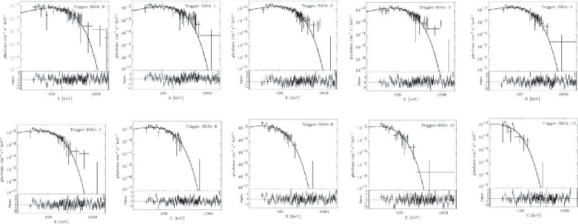
Figure 7: Same as fig. 4 but for burst 6504, for time bins: 1: 1.6 – 2.7 s, 2: 2.7 – 3.4 s, 3: 3.4 – 4.9 s, 4: 4.9 – 6.2 s, 5: 6.2 – 7.7 s, 6: 7.7 – 9.3 s, 8: 11.3 – 13.4 s, 10: 15.9 – 18.5 s, 12: 21.4 – 24.5 s.

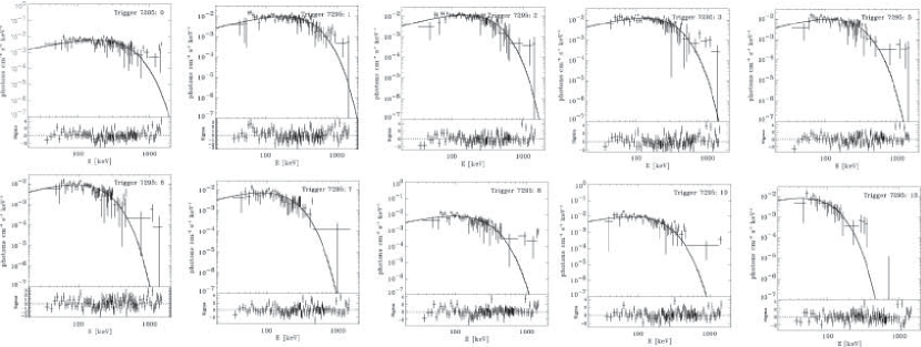
Figure 8: Same as fig. 4 but for burst 7295, for time bins: 0: 0 – 1.2 s, 1: 1.2 – 2.1 s, 2: 2.1 – 2.9 s, 3: 2.9 – 3.8 s, 5: 4.8 – 5.9 s, 6: 5.9 – 7.2 s, 7: 7.2 – 8.6 s, 8: 8.6 – 9.9 s, 10: 11.1 – 12.4 s, 13: 15.6 – 17.7 s.

As mentioned above, two of the five thermal pulses have an indication that there is a weak, additional, high-energy flux-component. In trigger 7295 (Fig. 8) the Rayleigh-Jeans portion of the spectrum fits the data well, but above $\sim$ 700 keV the data do not follow the exponential cutoff of the Wien portion. The photon flux remains constant at an approximate 5 % level of the maximum. Similarly, but somewhat less pronounced, there is extra flux at high energies in trigger 6504 (Fig. 7), mainly for the earliest time-bins. This could be due to Comptonization of the black body photons by the hot electrons, or it could be due to a separate non-thermal emission from synchrotron cooling of the electrons. We therefore re-fit these spectra with a two-component spectrum: a black body, representing the thermal emission, combined with a single power-law representing the non-thermal emission:

$$N_{E}(E,t)=A(t)\,(E/E_{\rm piv})^{s}$$ (7)

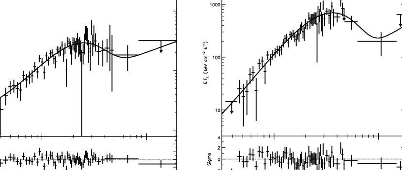
Figure 12: Combination of a black body and a single power-law fitted to time-resolved spectra of triggers 6504 (left panel) and 7295 (right panel). The digits following the trigger number correspond to the time bins in Figures 7 and 8, respectively. Note that the plot is in an $EF_{E}$ representation.

where $A$ is the amplitude in photons s^-1 cm^-2 keV^-1 and $E_{\rm piv}$ is a pivot energy in keV, and finally $s$ is the power-law index. We assume that the non-thermal emission, within the observed energy-band, can be represented by this power-law. Ideally, more elaborate models should be used for the non-thermal emission, such as a broken power law, with a peak representing the emission from the electrons with the lowest Lorentz factors. However, this is not permitted by the quality of the data, and therefore the power-law index represents an averaged value. On the other hand, we also note that for very efficient cooling the spectrum can be expected to be a power law of $\alpha=-3/2$ over the whole energy window. This is especially the case if there is no continuous heating during the emission episode. In Figure 12 one time bin for each of these two bursts are shown with fits to such a two-component model. Note that the spectra in the figure are in an $E\,F_{E}$ representation, i.e., energy flux per decade (unit: keV cm^-2 s^-1), to enhance the spectral energies with most energy flux output. From the figures it is evident that the two-component model can account for the high-energy flux as well, which a pure black body had problems with. The indices of the power-law component, for these fits, vary for 6504 from $s=-0.5$ to $-1.5$ and for 7295 it is constantly around $s=-0.9$, with somewhat large errors.

3.3.2 Bursts that are Initially Hard

Several authors have pointed out bursts which have hard spectra, consistent with black-body emission, for a short initial phase of the light curves, but which later become non-thermal. In Figure 2 the light curves of four such cases are shown and the phases during which the spectra are well fitted by black bodies are indicated. They are all medium-complex bursts. Trigger 6630 however looks like a single pulse, but it cannot be fitted with the pulse model by Kocevski, Ryde, & Liang (2003), which was shown to be able to fit most single pulses. This suggests that 6630 actually consists of several pulses which are heavily overlapped.

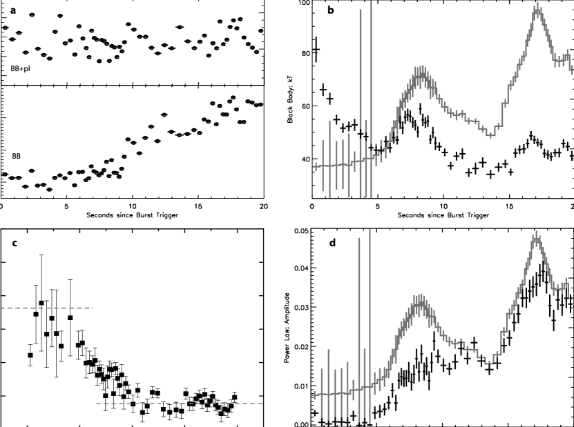
Figure 13: Analysis of trigger 5773. a) $\chi^{2}_{\nu}$ as a function of time for a black body (lower) and a black body and power law model (upper). b) Evolution of $kT$ plotted on top of the light curve (grey line), with the time resolution used in the analysis. c) The power-law index, $s$ as a function of time. The dashed lines show $s=-0.67$ (spectral-index for optically-thin synchrotron emission) and $s=-2.1$ (cooling spectrum). d) The amplitude of the power-law index grows in importance.

Inspired by the success of the two-component model in the study of the black-body pulses above, we continue by modelling these four triggers with such a model as well. The results of the analysis on trigger 5773 is shown in Figure 13. Only the first 20 seconds of the burst’s HERB data were recorded by BATSE, preventing us from a longer study. However, the main features are already present in these 20 s (which include the major part of the burst.) Panel a) in Figure 13 shows the time evolution of the $\chi^{2}_{\nu}$ -values for the two models: a pure black body and a combination of a black body and a power-law. For the first 5 seconds the black-body model gives reasonable $\chi^{2}_{\nu}$-values, after which the fit rapidly deteriorates. However, the two-component model is able to describe the data throughout. The temperature of the black body, in the two-component model, is depicted in panel b) where also the light curve is shown by the grey line. During the initial phase the temperature decreases monotonically, but rises again during the first major pulse. This is repeated for the second pulse. We note that the peak temperature precedes the peak in the light curve. The maximum temperature of the peaks also decreases, even though the intensity of the peaks increases. In panels c) and d) the evolution of the power-law component is shown. The power-law index varies from $\sim$ -0.7 down to $\sim$ -2.2. Assuming an optically-thin cooling model and that the single power-law averages such a spectrum, the first phase of the burst would be dominated by the spectrum below $E_{\rm p}$ having the value $-2/3$ (dashed line in the Figure). During the transition, which occurs at $\sim$ 10 seconds (i.e. during or somewhat after the first pulse), the smooth break in the non-thermal spectrum dominates in the observed band. Later, the synchrotron spectrum above $E_{\rm p}$ will dominate. In the fast cooling regime, the index of the power law of the electron distribution will be $-(p+2)/2$, where $p$ is the injected index, which for the Fermi type of particle acceleration in relativistic shocks is $p\sim 2.2$. This value gives a photon index of $s=-(p+2)/2=-2.1$ (dashed line in the Figure). Finally, panel d) shows that the amplitude of the power law grows in importance relative to the total emission, indicating again that the thermal emission component becomes increasingly swamped by the non-thermal radiation.

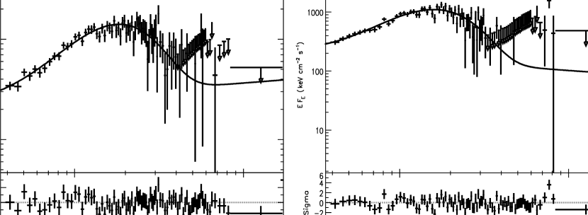
Figure 14: Time-resolved spectra of burst 6630 fitted with a two-component spectral model consisting of a black body and a power law. The time bins correspond to the times: $t=2.50-2.75$ s (left) and $t=2.75-3.1$ s. The fits require a power law with index $s=-1.9\pm 0.1$ and $-2.2\pm 0.2$, respectively. The upper-limit data-point at high energies represents the detector sensitivity.

A similar analysis was performed on trigger 6630. Ghirlanda et al. (2003a) demonstrated that the first $\sim$ 2 s are consistent with a black body and that the fits get worse thereafter. Here again the two-component model can indeed explain the data and the fits are good throughout the burst. To illustrate this we plot, in Figure 14, two time-resolved spectra which are beyond the initial black-body phase. Note again that the spectra in Figure 14 are in an $E\,F_{E}$ representation. These spectra are poorly fitted by a model consisting of a pure black body, which can be seen in Fig. 9 in Ghirlanda et al. (2003a), where both the $\chi^{2}$ as well as the residuals reflect the poor fit. However, as can be seen by the best fit for the two-component model, which is shown in Figure 14 by solid lines, such a model can describe the data. The $\chi^{2}_{\nu}$ for the two fits are now $\chi^{2}_{\nu}(dof)=0.81(105)$ and $0.995(105)$, respectively. Note, in particular, the improvement in the systematics of the residuals for the spectrum of time bin $t=2.75-3.1$ s, compared to the pure thermal fit in Ghirlanda et al. (2003a). Throughout the fit, the power-law index varies from $s=-1.1$ down to $s=-2.4$, suggesting that the power-law component is a synchrotron spectrum from the electrons above their minimum Lorentz factor.

A two-component model is also satisfactory for the initially hard triggers 829 and 1085, giving $\chi^{2}_{\nu}$ and residuals that are acceptable. The power-law indices vary from $s\sim-1.5$ to $\sim-2$, and $s\sim-1$ to $\sim-2$, respectively. We also note that Ghirlanda et al. (2003a) showed, for a few of their triggers, which were initially hard, that the early-time temperature decreases as $kT\propto t^{-1/4}$, consistent with the early power-law decays of the thermal pulses in the previous section. Finally, inspection of the light curves in Figure 2 suggests that the initial black-body behavior could be connected to a separate pulse. This is consistent with the picture that it represents a photospheric flash and the later, overlaid pulse(s) are from the non-thermal emission region. The analysis shows also that the photospheric temperature rises just before subsequent pulses, representing several different photospheres.

The interplay of the strengths of these two components will obviously affect the measured low-energy power-law of the spectrum, if it is modelled by a single GRB-function (eq.[1]). The variation of the component amplitudes will manifest itself as an evolution of the $\alpha$-parameter. Such a behavior has indeed been observed to occur in many bursts. This evolution therefore might simply reflect the relative strengths between the thermal and non-thermal components, and does not necessarily need to represent an actual change in radiative regime where the single electron emission pattern has to change, such as a change from self-absorbed to optically-thin synchrotron emission from the same emitting material. As the spectra in general are observed to soften with time, it would indicate that a thermal-dominated phase is followed by an increasing importance of the non-thermal component.

Finally, we note that the two-component model has four parameter, namely the black-body normalization, its temperature, and the power-law index and its normalization. It therefore has equal number of parameters as the GRB-function (Eq. 1).

4 Physical Interpretation

As suggested by the observations above, several spectral components probably are involved in the creation of the observed gamma-ray spectrum. Suggestions for the origin of the thermal component have been given both in the kinetic, fireball model and for electromagnetic models. To characterize the outflow we define the parameter $\sigma=L_{\rm P}/L_{\rm kin}$ as the ratio between the magnetic energy flux, or Poynting flux, and the kinetic energy flux. We first discuss our results within the fireball model (small $\sigma$) and later expand the discussion to also include large-$\sigma$ winds.

4.1 Fireball Model, small $\sigma$

In the fireball model the GRB emission stems from a highly relativistic wind with a low baryonic load. Large amounts of energy is assumed to be released at a small initial distance from the progenitor, $R_{0}$, and are injected into an optically thick, electron-positron pair wind (or shell). Several physical settings, where this could occur are plausible, but for long GRBs, it is now generally assumed that this occurs close to the center of a collapsing massive star. The wind is radiation-dominated and accelerates under its own pressure as a relativistic gas and, as it is opaque, the main part of the radiative energy is initially trapped. The opacity stems from the ambient baryonic electrons and the e^± pairs (the pairs naturally make a contribution only if they have not annihilated). During the expansion the fireball cools adiabatically, converting its internal energy into kinetic energy. Its Lorentz factor increases linearly (Mészáros, Laguna, Rees, 1993) until it reaches the saturation radius, $R_{\rm s}\sim R_{0}\eta$, where the dimensionless entropy of the wind is given by $\eta=L/\dot{M}c^{2}$ and describes the baryon load of the fireball (the initial radiation to rest-mass-energy ratio). Beyond this point all the thermal energy has been converted into kinetic energy of the out-flowing baryons, and the fireball coasts with constant Lorentz factor, $\Gamma=\eta$. The emission from this fireball is expected to be thermal. The opacity decreases while the fireball expands and the main part of the thermal radiation is emitted when the optical depth, $\tau$, is around unity. The transition time to optical thinness is relatively short, after which the emission becomes optically thin.

We will discuss two variations of the fireball model. One can imagine a continuous relativistic wind or one can focus on a single optically-thick shell and follow its emission as its expands.

4.1.1 Wind Model

A typical scenario in which a photospheric pulse can be created is the one described by a relativistic wind (Paczyński, 1990). The wind will have a photosphere at a radius and a temperature that are only dependent on the initial parameters of the flow. If one assumes a constant flow, the photospheric emission will be time-independent. For it to give rise to a pulse shape, the energy injection rate and/or the Lorentz factor have to change.

The wind photosphere is defined as the surface at a distance $R_{\rm w,ph}$ where $\tau_{\rm w}=1$. Above the photosphere the wind is optically thin. Let us calculate the optical depth through the whole wind measured along a ray towards the observer at infinity:

$$\tau(R_{\rm ph})=\int_{R_{\rm ph}}^{\infty}\,d\tau(R)=\int_{R_{\rm ph}}^{\infty}\frac{\rho^{\prime}\kappa dR}{{\cal{D}}(\mu)}.$$ (8)

$\kappa$ is the total mass opacity (per gram) due to the ambient electrons and the $e^{\pm}$ pairs, and the comoving density is given by

$$\rho^{\prime}=\frac{1}{\Gamma}\frac{\dot{M}}{4\pi R^{2}\beta c}.$$ (9)

Note that $\beta\Gamma\sim\Gamma$ for large $\Gamma$. The angle-dependent Lorentz factor ${\cal{D}}(\mu)\equiv[{\Gamma(1-\beta\mu)}]^{-1}$, takes care of the angular dependence of the optical depth (Abramowicz, Novikov, & Paczyński, 1991) in which $\theta=\rm{arccos}(\mu)$ is the angle between the direction of photon propagation and the matter velocity, which for small angles reduces to ${\cal{D}}=2\Gamma$. The upper limit in equation (8) represents integration through the whole wind. Solving this equation for $\tau=1$ gives that the wind photospheric radius is at

$$R_{\rm ph}=\frac{\kappa\dot{M}}{4\pi\beta c\Gamma{\cal{D}}(\mu)}\sim\frac{\kappa\dot{M}}{8\pi c\Gamma^{2}}$$ (10)

In the last step we used the fact that a typical burst $\Gamma$ is large and that $v\rightarrow c$. If the mass-injection rate is constant, then $R_{\rm ph}$ will remain constant and have a certain temperature, $kT(R_{\rm w,ph})$ and luminosity, $L_{\rm ph}\propto\dot{E}$. The temperature of the adiabatic, relativistic outflow depends on the radius as $kT(R)\propto R^{-2/3}$ (standard fireball model, Piran (1999)). To account for the temporal shape of a pulse one therefore has to assume a certain density profile in time of the wind or certain variations in the $\Gamma$ and/or $\dot{M}$. The location of the photosphere, and thereby the luminosity and temperature, has to be determined numerically. The observed shape of a pulse can then be used to deduce the history of the wind. In the pulse model of Daigne & Mochkovitch (2002), the rise phase of a pulse was attributed to a varying Lorentz factor. After the initial rise, the Lorentz factor remains constant and therefore also the intensity, until the end of the wind. Overlaid will be the non-thermal emission from the internal shocks, which together create the observed pulses.

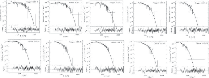
Figure 6: Same as fig. 4 but for burst 4157, for time bins: 0: 0.1 – 0.7 s , 1: 0.7 – 1.5 s , 2: 1.5 – 2.4 s, 3: 2.4 – 3.3 s, 4: 3.3 – 4.4 s, 5: 4.4 – 5.4 s, 6: 5.4 – 6.3 s, 7: 6.3 – 7.0 s , 9: 7.5 – 8.1 s, 20: 18.6 – 20.1 s.

To model a pure thermal pulse, including the decay phase, any of the other parameters have to be changed, for instance $\dot{M}$ can be varied. Then $\dot{M}$ has to grow approximately linearly to explain the observations above in Figure 11. The wind model also requires that $kT(R)\propto F(R)\propto R^{-2/3}$, that is, the ratio between temperature and flux, $kT/F$, is constant. A temporal variation in $kT$ will be followed by a similar variation in the flux. However, an increase of the temperature during the rise phase of the studied pulses above is not observed (see also Ghirlanda et al. (2003a)). A resolution to this could perhaps be the curvature effect. If it indeed is dominating, a monotonic flux-decay in the comoving frame (and thus a monotonic temperature decay), would have a pulse shape in the observer frame, see for instance figure 6 in Ryde & Petrosian (2002).

It is also plausible that the optical depths, and thus $R_{\rm ph}$ and $kT$, are different for different energies, which would lead to a multi-color black-body, decreasing the thermal appearance of the observed spectrum. On the other hand, Ryde & Svensson (2000) noted that several pulses have a break in their power-law decays, with the decay turning to a faster fall-off. In the wind model of Daigne & Mochkovitch (2002) such features are naturally explained and in the light curves that they produce, these features are indeed present, see their Fig. 6. Competing models therefore would have to explain these breaks as well. Here, we see such behaviors in the pulse of trigger 829, at 14 s, and in the pulse of 6630, at 5.5 s. These pulses are shown in Figure 2, in which the breaks are identified by the arrows.

In summary, the wind model does not provide an obvious reason for why the observed, fast temperature decays all seem to be narrowly distributed and tend to have a decay index of approximately $\sim-2/3$. However, more numerical investigations will be necessary.

4.1.2 Shell Model

We now study the following scenario. A hot, geometrically thin, fireball shell, with large optical-depth is ejected from the progenitor source into a low-intensity wind. The photosphere of the wind should be at small radii to ensure that the thermal shell emission occurs in an optical-thin environment of the wind, in order that it should be visible to an observer at infinity. From equation (10), $R_{\rm ph}$ is small if, for instance $\dot{M}$ is small and/or $\Gamma$ is large. The shell can still be optically thick, $\Delta\tau>1$, at the wind photosphere. For a shell with width, $\Delta R$, the optical depth is $\Delta\tau=(\kappa\dot{M}_{\rm sh}\Delta R)/(8\pi R_{\rm ph,w}^{2}\Gamma^{2}c).$ Moreover, we note that as long as the variations of the $\Gamma$ internally to the shell is not too large in relation to the width of the shell, it will not expand significantly from $\Delta R$ and behave as a section of a wind.

We now assume that the rise phase of the pulse can be attributed to the acceleration phase of the fireball, i.e. $R<R_{\rm s}$, with the energy flux $F\propto\Gamma^{k}$(t), to some power $k$, as well as to the effective emitting area. As the plasma is optically thick to its own electrons it is in principle an isentropic fluid which can be modelled as a gas with adiabatic index $\gamma=4/3$ (Rybicki & Lightman, 1979). We therefore have

$$kT^{\prime}\propto{\rho^{\prime}}^{\gamma-1}={\rho^{\prime}}^{1/3}$$ (11)

which is the adiabatic relation for electromagnetic radiation. Assuming a power law increase of the Lorentz factor, $\Gamma\propto t^{\xi}$

$$\rho^{\prime}\propto R^{-2}\Gamma^{-1}\propto t^{-(2+\xi)}$$ (12)

so that

$$kT=kT^{\prime}\,\Gamma\propto t^{\,2/3\,(\xi-1)}$$ (13)

If $\xi=1$, then the observed $kT$ is constant. The fits to the cases in Figure 11 indicate that $\xi$ has values from $0.6$ to $1.6$, see Table 3. In the numerical study by Mészáros, Laguna, Rees (1993), it was found that $\Gamma$ initially increases linearly at early stages of the evolution and later saturates (see their Fig. 3). The data here seem mainly to prefer a slower acceleration (we will later see that large-$\sigma$ models do indeed require such an acceleration). It is interesting to note that in the numerical modelling by Ruffini et al. (2003) (and references therein) the Lorentz factor increases linearly at a beginning but turns to a slower than linear increase after the pair fireball has interacted with the baryonic remnant of the progenitor star, before it saturates (their Fig. 9). The break-width parameter of the fitting function used here, $\delta$ (Eq. [6]) is of interest as it describes the transition from the linear increase of $\Gamma$ during the acceleration phase, to the saturated, coasting regime.

The break in the temperature decay is now reached at the saturation radius before the shell becomes optically thin. The photosphere of the fireball shell should then be at large distances from the progenitor to ensure that the emission is thermal throughout the whole evolution. From equation (10) we have that $R_{\tau=1}=10^{15}$ cm for large $R_{0}$ and low $\eta$ values. $10^{16}$ cm is a typical radius at which significant deceleration of the fireball has occurred as a result of the interaction with the interstellar medium and the onset of the afterglow (see, e.g. Rees & Mészáros (1992)). The optically-thick shell is cooling adiabatically due to the expansion and during the coasting phase ($\Gamma$ constant) the cooling of the shell will cause the intensity to drop and thus produce the decay phase of the pulse. The temperature changes as $kT^{\prime}\propto{\rho^{\prime}}^{1/3}$ (eq. [11]) and if the density of the wind decreases as $\rho\propto R^{-2}$ (eq. [9]), the adiabatic relation gives $kT\propto R^{-2/3}$. As $\Gamma$ is constant,

$$kT(t)\propto t^{-2/3}.$$ (14)

which corresponds to the observed temperature decays beyond the break.

A suggestion of such a scenario is given in Böttcher, Schlickeiser, & Marra (2001), who investigated the evolution of a pair fireball before and after it becomes optically thin. The collision-dominated pair phase results in the flash of thermal emission that is followed by the transition phase during which the fireball becomes Thomson thin, but the radiation remains dominated by thermal Comptonization. The initial thermal flash should typically be seen by BATSE, and could even be the main component. The flash from the optically thinning process would then be seen at higher energies, between 100 MeV and a few GeV, that is, much beyond the BATSE window. They find that the time for the fireball to become Thomson thin can be extended out to $\sim 1$ s and beyond depending on the total energy and the collimation (see their Fig. 1). The main characteristics of the observed pulses, can therefore, in principle, be reproduced.

An alternative to this scenario is, of course, that the thermal flash, emitted as the shell becomes optically thin, is detected in the BATSE range, instead. The break is thus reached during the acceleration phase as the transparency condition is met. Böttcher, Schlickeiser, & Marra (2001) showed that up to a few seconds after the initial explosion the pair plasma is still dominated by collisional processes and that the collision-less shocks, that are responsible for the non-thermal radiation, only occur after that turbulence has had time to form. This ensures that thermal character of the spectra. Grimsrud & Wasserman (1998) also showed that for a relativistic e^± pair wind the radiation field will be approximately black body out to $\tau<<1$ as long as $\Gamma\propto R$. If the optically thinning transition phase is reached as the fireball shell is still accelerating, the constancy in temperature during the rise phase can be explained, according to the above, and the decay is due to the interplay between the ongoing acceleration and the radiative emission, and detailed numerical simulations are needed, which again need to be able to explain the alleged preference of the -2/3–temperature drop. Furthermore, the modelling has to produce the peak energy at lower energies ($\sim$ 200 keV).

In summary, an optically-thick shell, expanding adiabatically, can reproduce the observed behavior, with the break in the temperature decay occurring at the saturation radius.

4.1.3 Additional Spectral Components and Additional Pulses

The above considerations were mainly for a purely thermal, single pulse. However, for a few of the investigated pulses there is an indication of a weaker, secondary, non-thermal spectral component as well as secondary pulses. We note again that the temperature rises in advance of the new pulse. Also, the non-thermal component becomes most important after the peak.

The typical photospheric radius is well before the radius at which the internal shocks occur $R\sim 3\times 10^{14}{\rm cm}\;(\Gamma/100)^{2}$, which is somewhat dependent on the initial distribution of the Lorentz factors. If the collisions occur mainly below the photosphere the outflow is more ordered in the optically-thin region and thus the shocks are less efficient, since the relative Lorentz factors are smaller. This could explain the absence of a non-thermal component in some pulses. Indeed, Kobayashi, Ryde, & MacFadyen (2002) showed that different amounts of variability of the shock emission can easily be found for varying initial set-ups. The non-thermal emission naturally arises in a time period after the thermal emission escapes, due to the time scale needed for turbulence to be created (Böttcher, Schlickeiser, & Marra, 2001), thereby explaining the delay. The initial section of a burst should bear the strongest signal of the photosphere.

Subsequent pulses could be due to the release of additional, optically thick shells from the central engine repeating the behavior. If the central engine emits another major shell which catches up the first one, they will collide and merge to temporarily form a single shell. The internal energy of the merged shell is the difference in kinetic energy before and after the collision. A significant fraction of the kinetic energy can therefore be converted into internal energy if the relative velocity is relativistic. The collision will thus re-energize the merged shell, heating it to higher temperatures and giving rise to the new thermal pulse in the light curve. A while later, synchrotron radiation is emitted due to the turbulence excited by the collision in the shell photosphere.

4.2 Poynting-Flux Models, Large $\sigma$

Most progenitor models for GRBs, include the formation of a rapidly rotating, compact object. Indeed, in the collapsar model in which the GRB is emitted when the iron core of a massive star collapses can very well produce a very rapidly rotating, highly magnetized, neutron star (Wardziński & Zdziarski, 2000). The magnetic field on such an object can be as high as $10^{16}$ G. The electromagnetic torque that such a field exerts on the compact object will partly decelerate its rotation on a time scale of seconds, and partly generate a strongly magnetized wind flowing at high Lorentz factors (see Uzov (1999) for a review). Such magnetic winds therefore naturally arise in most formation scenarios of GRBs. The importance of such a magnetic Poynting flux, $L_{\rm P}$, compared to the kinetic wind, $L_{\rm kin}$ (which is the luminosity in both e^±-pairs and radiation) is given by the $\sigma$-parameter, and $L_{\rm P}$ depends on high powers of the radius, magnetic field and the angular velocity of the compact object. For compact objects with a very high magnetic field, $\sigma$ is expected to be relatively large (Uzov, 1999). Also in electromagnetic models, the transformation of the out-flowing energy into gamma-rays is more efficient than in the kinetic models, and they naturally avoid heavy baryon loadings.

If the magnetic configuration of the rotating compact object is non-axisymmetric (such as the rotation of an inclined dipole) the resulting Poynting flux could very well be in the form of a striped wind, that is, the magnetic field is aligned transversely to the flow direction and changes sign on small length scales. Reconnection then creates a natural possibility for the local dissipation of the magnetic energy which is transferred to the matter. Apart from releasing energy, that can be radiated away and observed by a distant observer, this leads to a decrease in the magnetic energy with $R$, producing an outward gradient in the magnetic pressure, which is a source of acceleration of the flow. The rate of dissipation of the magnetic energy depends then on the reconnection rate of closely lying regions of different field line directions. Below the photosphere all the energy is deposited in the outflow and its adiabatic expansion. The acceleration here is slower than that in the fireball scenario, due to the continuous energy release; $\Gamma\propto R^{1/3}$ instead of the $\Gamma\propto R$, discussed above. As mentioned in §4.1.2 this is indeed what the temperature decay of most of the observed cases seem to indicate. The observed temperature of the thermal black-body emission from the photosphere is $kT=2\Gamma kT_{0}$, where $T_{0}\sim 2\times 10^{8}$ K $=17$ keV/k. The Lorentz factor at the photosphere then has to be $\sim 10$ to explain the observed peak energies in the previous section, which can be found for a somewhat less strong magnetic field. The saturation radius for the fireball model is where the terminal bulk Lorenz factor is reached. Such a radius also exists for a Poynting flux wind. As the rate of dissipation decreases due to the decreasing field strength, it eventually becomes slower than the expansion time-scale, and the dissipation terminates. The flow therefore ceases to accelerate and reached a final speed. After the out-flowing plasma has become optically thin and the magnetic field ceases to be frozen to the wind plasma (as the Goldrich-Julian density is reached) and large-amplitude electromagnetic-waves are created, in which the out-flowing particles are efficiently accelerated and emit non-thermal radiation.

Depending on where most of the energy is dissipated relative to the wind photosphere, the observed emission will be different, in much the same way as in the fireball discussion in the previous sections. In the detailed numerical modelling by Drenkhahn & Spruit (2002) of a Poynting flux wind, they illustrated the different scenarios by varying the $\sigma$-parameter. For low values most of the energy is converted into kinetic energy already before the photosphere. At medium values the thermal component becomes important. At most $\sim 17\%$ of the dissipatable magnetic energy is released as black-body emission. At higher $\sigma$, the main part of the magnetic energy is dissipated in the optically-thin region, and mainly non-thermal radiation is observed. Therefore, such a wind will also naturally produce several components in the observed spectrum, with variable relative strength (see also Lyutikov & Usov (2000)).

Drenkhahn & Spruit (2002) further showed that the main properties of the emission essentially depend on the ratio between the saturation radius and the photospheric radius. The black-body component will be most important when these two radii coincide. This means that if we see black-body emission dominating the spectrum, as in the observed cases above, we are probably seeing outflows in which the black-body emission is maximally important and thus the saturation and photosphere radii are similar. In such a set-up the initial Poynting flux is of the order of 40 times larger than the kinetic energy. The wind accelerates with $\Gamma\propto R^{1/3}$ up to the point where the photons escape, at the photosphere. This model could thus overcome the problems in the previous section, in which it was assumed that the saturation radius was reached in the optically-thick region, which makes the emission inefficient. Here, instead, as the saturation and the photospheric radii coincide, the peak emission does indeed emanate from the photosphere. Also, inserting $\xi=1/3$ in equation (13) we obtain $kT\propto t^{-4/9}$ which is steeper than in the fireball model and might be a better description of the early temperature decays, most notably, trigger 2193. These features make the Poynting flux model attractive to explain the observations, even though a final answer will need to include more detailed modelling, beyond the scope of this paper.

Secondary pulses of the light curve, in this model, might be due to secondary outbursts from the central engine. If the properties of the second outburst are different from the first one, for instance a decreasing $\sigma$-ratio (maybe by the baryon ’pollution’ increasing with time), the photosphere could be reached at larger distances and the temperature of the thermal radiation will then be lower, explaining this property in the observations. Also, the non-thermal emission, that stems from the dissipation in the optically-thin regions through reconnections happening beyond the photosphere, will be emitted with a small time delay compared to the thermal emission. This is what is observed.

In summary, similarly to the shell model, this model can explain the observed behavior. In this case the saturation radius and the photosphere coincide. Furthermore, a slower acceleration can reproduce the finite temperature decay slopes before the break.

5 Discussion and Conclusions

There are two important regions in the relativistic outflow that produce the high-energy emission in GRBs: the thermal photosphere and the region in the wind emitting non-thermal radiation. This leads to multiple components in the light curve and spectra of GRBs. We have identified a few simple GRB pulses which are consistent with an intrinsic black-body emission. It is therefore natural to interpret these exceptionally hard pulses as being emission from the wind (or shell) photosphere. Most of these bursts have good black-body fits throughout their evolution. In two cases, however, (triggers 6504 and 7295), there is evidence of a weak, non-thermal component. Furthermore, there are other, medium complex, bursts with an initial thermal phase and a later phase that is non-thermal. An example of such a burst is trigger 6630. We have shown that a two-component, hybrid model can indeed describe all these bursts throughout their evolution. Several theoretical models predict such a two-component spectrum. Furthermore, Comptonization of the black-body component could explain the extra flux at high energies. However, as we have shown, the two-component model can explain the softening of $\alpha$, which Comptonization would fail to do. We also found that the temperature decay is a monotonic function, that can be modelled by a broken power-law with an initially flat or weak decay turning into a faster decay. All bursts are consistent with a sharp break and a decay of $-2/3$.

Our interpretation is therefore the following. The spectra and light curves of all GRBs consist of several components, a black body and a non-thermal one with variable relative strengths. In the five pulses in our main analysis, the black-body emission dominates throughout the pulse. The non-thermal components are weak or are not seen in the gamma-ray band. However, for other cases the black-body component will be invisible or seen only in the initial phase of the light curve.

McQuinn, Ryde, & Petrosian (2004, in prep.) studied the curvature effect and found that it can have a substantial effect on the light curve, while its effect on the spectra is smaller. Our spectral analysis presented here should therefore not be heavily affected by this effect. They further find, as mentioned above, that the curvature effect is more important on the light-curves of thermal pulses compared to non-thermal pulses, even though their spectra are not strongly altered. We therefore concentrated our present study on the behavior of the temperature $kT$. Compared to the photon flux (e.g. in Fig. 13b,d) it also has several simplifying advantages. The measurements do not suffer as much from additional flux components and band width problems. We postpone the detailed analysis of the light curves, including all important physical effect, to a later paper.

One could argue that as the Rayleigh-Jeans portion of the spectrum is no longer visible for some of the late-time spectra, it might be dangerous to interpret these fits. This happens, for instance, for the latest time-bins in triggers 3256 and 4157. As we are not recording the spectrum beneath the energy threshold, it may very well not be a Rayleigh-Jeans tail anymore. However, as the study above has shown, when the spectrum starts to differ significantly from a black body, the change will be visible mainly at the highest energies. Thus, if the low-energy spectrum were altered, a change in the Wien-portion of the spectrum, which is in the observable range, would also be detected. Especially in a $EF_{E}$ representation the high-energy component will show up markedly. Therefore, we argue that the black-body fits can be trusted even though, for some spectra, most of the Rayleigh-Jeans portion is out of the band.

It has also been made clear that a high temporal resolution is vital for spectroscopic studies. Due to the spectral evolution of the spectrum during the pulse, the time-integrated spectrum will not necessarily reflect the instantaneous spectrum, which is the one bearing the direct consequence of the physical creation process(es). This was shown in the comparison between the fits in Table 2 and the instantaneous fits. The connection between the instantaneous spectra and the time-integrated spectra is, in general, well understood and is prescribed by the spectral, empirical relations, as discussed by Ryde & Svensson (1999).

The study presented here has illustrated the risks of interpreting fits made to BATSE data. In general, fits are made using the GRB function (eq. [1]) and the resulting parameters are then interpreted. The first issue that has to be noted is that the low energy power-law, $\alpha$, is the asymptotic power-law index and that the spectrum within the BATSE band seldom reaches this power law and comprises mainly the curved section below the peak energy. The $\alpha$–value therefore does not need to reach $\alpha=+1$, which would be the criterium to identify a black-body spectrum. This is the case in particular for black-body spectra which have such a low $kT$ that the Rayleigh-Jeans part of the spectrum is not fully detected. It is therefore risky to directly interpret results, found by using the GRB-function, in terms of radiation processes. As demonstrated above, the correct approach is to fit the data directly with a Planck function (maybe in combination with other components), which is then used in the forward-folding, deconvolution-process, and thereafter interpret the results of the fit. Also, as evident from the fits, an artificial softening of the spectra would be detected, if they were to be fitted with the GRB function. This is, for instance, evident for trigger 4157 in Figure 6. The reason for this effect is, again, that the black body moves out of the detector’s limited energy window. Also an apparent softening can be caused by a changing relative strength between the hard, black-body emission and the power-law, non-thermal emission. Moreover, it is also important to point out that the black body is a physical model while the GRB function is merely an empirical model.

As illustrated in Fig. 3 the conclusive evidence for a black body, namely the $\alpha=+1$ power-law is not completely reached for the BATSE pulses. Further observations of very hard spectra by, for instance, Swift’s BAT ($\sim 15-150$ keV) will be able to better prove the nature of the emission process. However, the triggering systems of detectors are such that the observed spectra have peaks mainly concentrated within their energy band. Therefore, a very high peak-energy case, with a large interval, within which $\alpha$ can be measured, will by necessity be rare. We have further argued that a non-thermal emission component should normally accompany the thermal one. Therefore, below a certain energy the low-energy component will still be dominated by the non-thermal emission. Rather than focusing on the $\alpha$-value, a broad band detection by, for instance the Gamma-Ray Large Area Space Telescope (GLAST), or, even better, a combination of Swift and GLAST, will therefore be powerful in testing further the observations and suggestions presented here. GLAST, which is scheduled to be launched in year 2007, will have a full spectral coverage from approximately 10 keV up to $\sim$ 200 GeV, by combining its gamma-ray bursts monitor (GBM), and its large area telescope (LAT). As the observations above suggest, there are synchrotron components with peak energies higher than $\sim$ 1 MeV in several cases. The full spectral coverage of GLAST will give better possibilities in fitting both the thermal and the non-thermal components and studying their relative behaviors. Furthermore, if the pulse is indeed due to the thermal emission from the optically-thick shell, as described above, it must needs be accompanied by a flash at higher energies. This would be detectable by the GLAST satellite with the combination of the GBM, seeing the thermal, optically thick pulses and maybe the non-thermal component, and the LAT, seeing the emission from the optically thinning phases. Such observations will give a possibility to test these models.

Table 1: Bursts Discussed in the Text

Burst	Trigger	LAD	$t_{\rm m}$
Name			[s]
910927	829	4	3.5
911118	1085	4	6.0
930214	2193	1	10.7
941023	3256	7	1.6
951228	4157	7	7.8
970111	5773	0	17.2
971127	6504	2	3.1
980306	6630	3	1.8
990102	7295	3	2.2

Table 2: Averaged Spectral Properties of the Burst Sample Using the GRB Model

Trigger	$C$	$\alpha$	$\beta$	$E_{\rm p}$
	[photons/s/cm2/keV]			[keV]
829	$0.095\pm 0.005$	$-0.03\pm 0.05$	$-4.0\pm 0.2$	$122.9\pm 1.1$
1085	$0.155\pm 0.003$	$-0.65\pm 0.02$	$-2.95\pm 0.05$	$209\pm 2$
2193	0.0140 $\pm$ 0.0010	0.53 $\pm$ 0.10	$-2.76\pm$ 0.18	269 $\pm$ 9
3256	0.008 $\pm$ 0.001	$-1.03\pm$ 0.13	$-\infty$	152 $\pm$ 9
4157	0.11 $\pm$ 0.03	0.10 $\pm$ 0.19	$-3.6\pm$ 0.3	72.2 $\pm$ 1.4
5773	$0.131\pm 0.002$	$-0.17\pm 0.02$	$-4.6\pm 0.4$	$185.1\pm 1.1$
6504	0.017 $\pm$ 0.003	$-0.2\pm$ 0.2	$-3.4\pm$ 1.4	179 $\pm$ 14
6630	$0.092\pm 0.002$	$-0.52\pm 0.03$	$-\infty$	$283\pm 5$
7295	0.0175$\pm$ 0.0013	0.58 $\pm$ 0.12	$-2.8\pm$ 0.2	341 $\pm$ 16

Table 3: Temperature Evolution

Trigger	$kT_{\rm n}$	$a$	$b$	$\delta$	$t_{0}$
	[keV]				[s]
2193	$86.4\pm 1.2$	$-0.25\pm 0.02$	$-0.78\pm 0.04$	$0.15$	$12.9\pm 1.1$
	$86.2\pm 1.7$	$-0.26\pm 0.02$	$-0.67$	$0.01\pm 0.15$	$11.0\pm 0.6$
3256	$17.5\pm 0.5$	$-0.16\pm 0.04$	$-0.69\pm 0.04$	$0.15$	$2.3\pm 0.3$
4157
comp 1	$6.5\pm 1.4$	$0.4\pm 0.2$	$-0.8\pm 0.1$	$0.0\pm 0.1$	$0.67\pm 0.06$
comp 2	$13\pm 2$	-”-	-”-	-”-	$7.8\pm 0.5$
6504	$28.4\pm 0.6$	$-0.11\pm 0.09$	$-0.67\pm 0.07$	$0.16\pm 0.18$	$3.8\pm 0.6$
7295	$41.2\pm 1.3$	$-0.12\pm 0.06$	$-0.74\pm 0.04$	$0.15$	$3.3\pm 0.5$
	$41.8\pm 1.3$	$0.04\pm 0.21$	$-0.67$	$0.2\pm 0.2$	$2.17\pm 0.7$

Figure 1: Light curves of the five thermal pulses used in the study. The pulses have hard spectra and are modelled with black-body spectra.

Figure 3: Spectral distributions of various emissions with a hard, low-energy, slope in a $E\,F_{E}$-representation; Planck spectrum (solid line), Wien spectrum (dashed), optically-thin thermal-synchrotron (dotted), and small-pitch angle synchrotron emission from a soft energy-distribution of relativistic electrons (dot-dashed). The latter spectrum can approximately represent a Compton-attenuated synchrotron-spectrum, as well. The spectra are normalized to each other to facilitate a comparison. The typical BATSE energy window is also indicated.

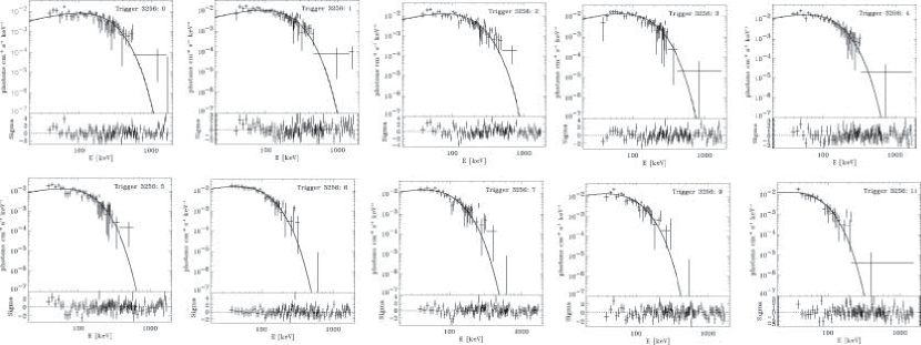
Figure 5: Same as fig. 4 but for burst 3256, for time bins: 0:0 – 0.8 s , 1: 0.8 – 1.5 s , 2: 1.5 – 2.2 s, 3:2.2 – 1.9 s, 4:2.9 – 3.6 s, 5: 3.6 – 4.5 s, 6: 4.5 – 5.4 s, 7: 5.4 – 6.3 s, 9: 7.4 – 8.6 s, 11: 9.9 – 11.3 s.

Figure 9: Reduced $\chi^{2}$-values, $\chi^{2}_{\nu}$, for the time-resolved spectra of the burst studied in the text. The dashed line is the reduced $\chi^{2}$-value for the total fit.

Figure 11: Black-body temperature, $kT$, in the observer frame, as a function of time. Single, broken, power-law functions (eq.[6]) have been fitted to all pulses except trigger 4157, for which a sum of two, broken, power-laws has been fitted. The breaks in the figures correspond to the breaks in the light curves in Figure 1. The solid lines correspond to fits with $\delta=0.15$, while the dashed curves are the best fits with $b=-0.67$. See the text and Table 3 for details.

References

- Abramowicz, Novikov, & Paczyński (1991) Abramowicz, M. A., Novikov, I. D., Paczyński, B. 1991, ApJ 369, 175
- Band et al. (1993) Band, D., et al. 1993, ApJ, 413, 281
- Blinnikov et al. (1999) Blinnikov, S., et al. 1999, Astr. Rep., 43, 739
- Böttcher, Schlickeiser, & Marra (2001) Böttcher, M., Schlickeiser, R., & Marra, A. 2001, ApJ 563, 71
- Crider et al. (1997) Crider, A., et al. 1997, ApJ, 479, L39
- Daigne & Mochkovitch (2002) Daigne, F. & Mochkovitch, R. 2002, MNRAS, 336, 1271
- Dermer & Boettcher (2000) Dermer, C. & Böttcher, M. 2000, ApJ, 534, L155
- Drenkhahn & Spruit (2002) Drenkhahn, G., & Spruit, H. C. 2002, A&A, 391, 1141
- Fishman et al. (1989) Fishman, G. J., et al. 1989, in Proc. of the GRO Science Workshop, ed. W. N. Johnson, 2
- Ghirlanda et al. (2003a) Ghirlanda, G., Celotti, A., & Ghisellini, G. 2003, A&A, 406, 879
- Ghisellini et al. (2000) Ghisellini, G., Lazzati, D., Celotti, A., & Rees, M. J. 2000, MNRAS, 316, L45
- Gradshteyn & Ryzhik (1965) Gradshteyn, I. S., & Ryzhik, I. M. 1965, Table of Integrals, Series, and Products (New York: Academic Press)
- Grimsrud & Wasserman (1998) Grimsrud, O. M., & Wasserman, I. 1998, MNRAS, 300, 1158
- Kaneko et al. (2004) Kaneko, Y., Preece, R. D., Gonzalez, M. M., Dingus, B. L., & Briggs, M. S. 2004, in the proceedings of ”Astrophysical Particle Acceleration in Geospace and Beyond”, Chattanooga, 2002, AGU monograph
- Kocevski, Ryde, & Liang (2003) Kocevski, D., Ryde F., & Liang E., 2003, ApJ, 596, 389
- Kobayashi, Ryde, & MacFadyen (2002) Kobayashi, S., Ryde F., & MacFadyen, A., 2002, ApJ, 577, 302
- Kobayashi & Sari (2001) Kobayashi, S., & Sari, R. 2001, ApJ, 542, 819
- Liang (1997) Liang, E. P. 1997, ApJ, 491, L15
- Lloyd-Ronning & Petrosian (2000) Lloyd-Ronning, N. & Petrosian, V. 2000, ApJ, 543, 722
- Lyutikov & Usov (2000) Lyutikov, M. & Usov, V. V. 2000, ApJ, 543, L129
- Mészáros (2002) Mészarós, P. 2002, ARA&A, 40, 137
- Mészáros et al. (2002) Mészarós, P., Ramirez-Ruiz, E., Rees, M. J., & Zhang, B. 2002, ApJ, 578, 812
- Mészáros, Laguna, Rees (1993) Mészarós, P., Laguna, P.,& Rees, M. J. 1993, ApJ, 415, 181
- Mészáros, & Rees (2000) Mészarós, P.,& Rees, M. J. 2000, ApJ, 530, 292
- Pacholczyk (1970) Pacholczyk, A. G. 1970, Radio Astrophysics (San Francisco: W. H. Freeman and Co.)
- Paczyński (1990) Paczyński, B. 1990, ApJ, 363, 218
- Petrosian (1981) Petrosian, V. 1981, ApJ, 251, 727
- Piran (1999) Piran, T. 1999, Physics Reports, 314, 575
- Planck (1901) Planck, M. 1901, Ann. Physik, 4, 553
- Preece et al. (1998) Preece, R. D., Briggs, M. S., Mallozzi, R. S., Pendleton, G. N., Paciesas, W. S., & Band, D. L. 1998, ApJ, 506, 23
- Preece et al. (2000) Preece, R. D., Briggs, M. S., Mallozzi, R. S., Pendleton, G. N., Paciesas, W. S., & Band, D. L. 2000, ApJSS, 126, 19
- Rees & Mészáros (1992) Rees, M. J., & Mészáros, P. 1992, MNRAS, 258, 41
- Ruffini et al. (2001) Ruffini, R., Bianco, C. L., Fraschetti, F., Xue, S., & Chardonnet, P. 2001, ApJ, 555, L113
- Ruffini et al. (2003) Ruffini, R., Bianco, C. L., Xue, S., Chardonnet, P., & Fraschetti, F. 2003, IJMPD, 12, 173
- Rybicki & Lightman (1979) Rybicki, G. B., & Lightman, A. P. 1979, Radiative Processes in Astrophysics (New York: Wiley)
- Ryde (1999) Ryde, F. 1999, Astro. Lett. and Comm., 39, 281
- Ryde & Petrosian (2002) Ryde, F., & Petrosian, V. 2002, ApJ, 578, 290
- Ryde & Svensson (2000) Ryde, F., & Svensson, R. 2000, ApJ, 529, L13
- Ryde & Svensson (1999) Ryde, F., & Svensson, R. 1999, ApJ, 512, 693
- Stern & Poutanen (2004) Stern, B. & Poutanen, J. 2004, MNRAS, in press
- Uzov (1999) Uzov, V. V., in ASP Conf. Ser, 190, Gamma-Ray Bursts: The First Three Minutes, Ed. J. Poutanen & R. Svensson (San Francisco: ASP), 153
- Wardziński & Zdziarski (2000) Wardziński, G. & Zdziarski, A. A. 2000, MNRAS, 314, 183