Properties of the warm magnetized ISM, as inferred from WSRT polarimetric imaging

We describe a first attempt to derive properties of the regular and turbulent Galactic magnetic field from multi-frequency polarimetric observations of the diffuse Galactic synchrotron background. A single-cell-size model of the thin Galactic disk is constructed which includes random and regular magnetic fields and thermal and relativistic electrons. The disk is irradiated from behind with a uniform partially polarized background. Radiation from the background and from the thin disk is Faraday rotated and depolarized while propagating through the medium. The model parameters are estimated from a comparison with 350 MHz observations in two regions at intermediate latitudes done with the Westerbork Synthesis Radio Telescope. We obtain good consistency between the estimates for the random and regular magnetic field strengths and typical scales of structure in the two regions. The regular magnetic field strength found is a few $\mu$G, and the ratio of random to regular magnetic field strength $B_{ran}/B_{reg}$ is 0.7 $\pm$ 0.5, for a typical scale of the random component of 15 $\pm$ 10 pc. Furthermore, the regular magnetic field is directed almost perpendicular to the line of sight. This modeling is a potentially powerful method to estimate the structure of the Galactic magnetic field, especially when more polarimetric observations of the diffuse synchrotron background at intermediate latitudes become available.

1 Introduction

Since the first interpretation of small-scale structure in the linearly polarized component of the Galactic synchrotron background as being due to Faraday rotation (Wieringa et al. 1993), many observations of the Galactic synchrotron emission have shown intricate structure in polarization on many scales, often unaccompanied by structure in total power. Although it has been recognized that the Faraday rotation and depolarization of the polarized synchrotron emission are due to small-scale fluctuations in the Galactic magnetic field, thermal electron density and/or the line of sight, a quantitative description of this structure has proven to be extremely difficult. This is because depolarization arises both along the line of sight and in the plane of the sky (i.e. within the telescope beam), whereas the rotation measure $RM$ is an integral over the line of sight of thermal electron density $n_{e}$ and Galactic magnetic field along the line of sight $B_{\parallel}$: $RM[\mbox{rad\leavevmode\nobreak\ m}^{-2}]=0.81\int\,n_{e}[\mbox{cm}^{-3}]\,B_{\parallel}[\mu\mbox{G}]\,ds[\mbox{pc}]$.

Use of the diffuse Galactic synchrotron emission as a tracer of the Galactic magnetic field is complementary to the magnetic field estimates derived from pulsars (e.g. Rand & Kulkarni 1989, Ohno & Shibata 1993) and extragalactic radio sources (e.g. Simard-Normandin & Kronberg 1980, Clegg et al. 1992, Brown et al. 2003), in that the diffuse background can provide a continuous field of RMs on scales from the field size down to the resolution of the observation. Therefore this is a unique method to infer scales and amplitudes of fluctuations in the Galactic magnetic field and the electron density.

The RM of the synchrotron background has been used to determine the nature of distinct objects (Gray et al. 1998, Uyanıker & Landecker 2002, Haverkorn et al. 2003a), to estimate the uniform component of the Galactic magnetic field (Haverkorn et al. 2003b) or the magnetic field strength and structure in supernova remnants (Uyanıker et al. 2002), and to infer the polarization horizon (Uyanıker et al. 2003). However, to the authors’ knowledge, this is the first attempt to derive the turbulent component of the magnetic field (not associated with any discrete structure) from the diffuse synchrotron background.

In this paper, we present a simple model of the Galactic thin disk as a synchrotron emitting and Faraday-rotating medium, consisting of cells with a certain electron density and magnetic field. We compare the model predictions with observed properties of the linear polarization in two fields observed with the Westerbork Synthesis Radio Telescope (WSRT), to derive estimates for several physical parameters of the warm ISM. In Sect. 2 we discuss the WSRT polarization observations that will be used to compare to the model. Section 3 describes depth depolarization in a layer that contains both synchrotron-emitting and Faraday-rotating material. We discuss in Sect. 4 the ingredients of a model for a thin disk, combined with a thick disk or halo providing a constant polarized background. In Sect. 5 we will describe the model in some detail, and how observational constraints can be used to derive estimates for parameters like the magnetic field strength and direction. In Sect. 6 we apply the model to our observations and discuss its results. Finally, we present a summary and conclusions in Sect. 7.

2 The observations

	Auriga	Horologium
(l,b)	(161${}^{\mbox{\tiny o}}$, 16${}^{\mbox{\tiny o}}$)	(137${}^{\mbox{\tiny o}}$, 7${}^{\mbox{\tiny o}}$)
size	7${}^{\mbox{\tiny o}}$$\times$9${}^{\mbox{\tiny o}}$	7${}^{\mbox{\tiny o}}$$\times$7${}^{\mbox{\tiny o}}$
FWHM	5.0′$\times$6.3′	5.0′$\times$5.5′
pointings	5$\times$7	5$\times$5
bandwidth	5 MHz	5 MHz
frequencies	341, 349, 355, 360, 375 MHz

Table 1: WSRT polarization observations in the constellations Auriga and Horologium. Given are position and size of each region, the resolution, the number of pointings used to mosaic the region, the frequency bandwidth and the central frequency in each band.

Two fields of observation in the constellations Horologium and Auriga, described in detail in Haverkorn et al. (2003a, 2003b) are used to estimate parameters of the depolarization model. Observations out of the Galactic plane are used to avoid discrete objects like supernova remnants and H ii regions, which would skew the statistical information of the radiation that we use. Relevant properties of the observations are given in Table 1. Undetected large-scale components in Stokes $Q$ and $U$ are not thought to be important in these fields around 350 MHz (Haverkorn et al. 2004).

Fig. 1 shows the linearly polarized intensity $P=\sqrt{Q^{2}+U^{2}}$ of the two regions in grey scale. The structure in $P$ is uncorrelated with total intensity $I$, which does not show any structure on scales visible to the interferometer down to noise level. Rotation measures $RM$ were derived from the polarization angle $\phi=\phi_{0}+RM\lambda^{2}$, where the ambiguity in $\phi$ over $n\,180\mbox{${}^{\mbox{\tiny o}}$}$ has been taken into account (Haverkorn et al. 2003b). $RM$ maps are shown as circles in Fig. 1. The $RM$ in the Auriga region (left) shows a gradient of about 1 rad m^-2 per degree in the direction of position angle $\theta=-20\mbox{${}^{\mbox{\tiny o}}$}$ (N through E).

The linear $\phi(\lambda^{2})$-relation can be destroyed by depolarization, which yields incorrect $RM$ values. Therefore, we only consider “reliably determined” $RM$ values, where “reliable” is defined by (a) the reduced $\chi^{2}$ of the linear $\phi(\lambda^{2})$-relation $\chi^{2}_{red}<2$, and (b) the polarized intensity averaged over frequency $\left<P\right>>20$ mJy/beam ($\sim 4$ – $5\sigma$).

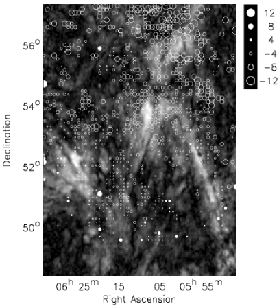
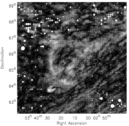
Figure 1: RM maps of the observed regions in Auriga (left) and in Horologium (right), overlaid on polarized intensity at 349 MHz in grey scale. White denotes high polarized intensity, with a maximum of 95 mJy/beam. RMs are denoted by white circles, and filled circles are positive $RM$s. The diameter of the symbol represents the magnitude of $RM$, where the scaling is given in rad m^-2. Only $RM$s for which $\langle P\rangle\geq 5\sigma$ and reduced $\chi^{2}$ of the linear $\phi(\lambda^{2})$-relation $<2$ are shown, and only every second synthesized beam.

Figure 2: Histograms of (from top to bottom) $Q$, $U$ and $I$ for 5 frequencies, and $RM$ for Auriga (left) and Horologium (right). Data of $Q$, $U$ and $I$ are 5 times oversampled, and only reliably determined $RM$s are included. In the solid line histogram of $RM$ in the Auriga region, the $RM$ gradient over the region is subtracted; the dashed line gives the histogram of the observed $RM$ including the gradient.

Histograms of the distributions of Stokes parameters $Q$, $U$ and $I$, and of $RM$ are given in Fig. 2 for Auriga (left) and Horologium (right). In the $I$ map, point sources were subtracted down to 5 mJy/beam. For $Q$, $U$ and $I$, data from all five frequencies are shown in the same plot. The $RM$ plot of the Auriga region contains the distribution of observed $RM$ (dashed line), as well as that of $RM$ where the best-fit linear gradient in $RM$ has been subtracted (solid line). The statistical information along these two separate lines of sight will be used in Sect. 6 to infer information on the Galactic magnetic field and correlation lengths in the warm ionized ISM.

3 Depth depolarization

The absence of correlated structure in $I$ appears to be a general feature: both regions discussed here show it, as do other observations made with the WSRT at frequencies around 350 MHz (e.g. Katgert & de Bruyn 1999, Schnitzeler et al., in prep). The lack of corresponding structure in $I$ suggests that Faraday rotation is the main process responsible for the observed structure in polarization.

However, rotation of the polarization angle cannot by itself cause structure in $P$. As shown in Haverkorn et al. (2004), the structure in $P$ in the observations discussed here cannot be caused by a missing large-scale structure component. Instead, depolarization must be the main creator of fluctuations in $P$. Depolarization can essentially occur in three ways: along the line of sight, in the plane of the sky or within the frequency band. As the latter process only causes significant depolarization for bandwidths much wider than those used here, we will ignore bandwidth depolarization. Depolarization along the line of sight is referred to here as depth depolarization (a combination of internal Faraday dispersion and differential Faraday rotation (Sokoloff et al. 1998, Fletcher et al. 2004)), as it occurs due to averaging of polarization angles along the line of sight. In addition, a finite width of the telescope beam can cause beam depolarization if the structure in polarization angle is on scales smaller than the beam. Beam depolarization is clearly observed in the fields discussed here, but it cannot explain the structure on scales larger than that of the beam (Haverkorn et al. 2004).

We are therefore led to consider the situation in which the medium that produces the Faraday rotation is mixed with a medium that emits synchrotron radiation, which produces structure in $P$ through depth depolarization. The low level of small-scale structure in $I$ in all of these observations implies that the total intensity of the synchrotron emission must be very uniform. However, the magnetic field, and therefore the synchrotron emissivity of the thin disk, is far from uniform (e.g. Beck et al. 1996, Han & Wielebinski 2002). Therefore, the smoothness of the synchrotron total intensity cannot be due to homogeneous synchrotron emission. Instead, the number of turbulent cells along the line of sight must be so large that the spatial variation in synchrotron emissivity, which is a scalar quantity, is averaged out. Linear polarization is a vector, so that small-scale structure is more easily preserved. Furthermore, total intensity is integrated over a much larger path length than polarized intensity because it isn’t depolarized. Finally, in the second quadrant, where our observations were done, the perpendicular component of the uniform Galactic magnetic field is believed to dominate the component parallel to the line of sight (e.g. Beck 2001). This means that $B_{\perp}$, and therefore the emitted synchrotron radiation, has a large uniform component.

4 Relevant components of the ISM

4.1 Cosmic rays and thermal gas

The synchrotron intensity is the integrated non-thermal emission along the line of sight. The intensity depends on the relativistic electron density $n_{e,rel}$ and magnetic field perpendicular to the line of sight $B_{\perp}$. Beuermann et al. (1985) have modeled the Galactic synchrotron emissivity $\varepsilon$ from the continuum survey by Haslam et al. (1981, 1982) at 408 MHz. They incorporate spiral structure in the synchrotron radiation and find two components of emission, viz. a galactocentric thick and thin disk with half equivalent widths of $h_{\varepsilon,b}\approx 1800$ pc and $h_{\varepsilon,n}\approx 180$ pc at the radius of the Sun, respectively, for a galactocentric radius of the Sun $R_{\odot}=10$ kpc. This corresponds to an exponential scale height of $h_{syn,thick}\approx 1500$ pc and $h_{syn,thin}\approx 150$ pc scaled to a galactocentric radius of the Sun $R_{\odot}=8.5$ kpc (Beck 2001). Note that the scale heights of the cosmic-ray electrons and of the magnetic field must be larger than that of the synchrotron disk, e.g. by factors 2 and 4 in case of equipartition (Beck 2001).

The major part of the Faraday rotation is caused by the warm ionized medium, contained in the so-called Reynolds layer (Reynolds 1989, 1991). The layer has a height of about 1 kpc, a temperature $T\approx$ 8000 K, and a thermal electron density concentrated in clumps of $n_{e,th}\approx 0.08$ cm^-3 with a filling factor of about 20%.

In this paper we will consider two domains in the ISM. The first domain is the thin synchrotron disk, which coincides with the stellar disk ($\sim 200-300$ pc), the thin H i disk ($\sim$ 200 pc, Dickey & Lockman 1990), and the disk of classical H ii regions ($\sim$ 60 pc). The second domain is the Reynolds layer, which coincides with the thick synchrotron disk. There is depolarization in both domains. The Local Bubble and Local Interstellar cloud contributions to the $RM$ are so small that they are neglected here.

4.2 Regular and random Galactic magnetic field

We decompose the Galactic magnetic field in a regular large-scale component and a random component ${\bf B=B}_{reg}+{\bf B}_{ran}$. Estimates of the ratio of random to regular magnetic field strengths $B_{ran}/B_{reg}$ in the literature seem to depend on the method used. Magnetic field determinations using $RM$s from extragalactic sources yield $B_{ran}/B_{reg}\approx 0.5-1$ (Jokipii & Lerche 1969, Clegg et al. 1992). Pulsar $RM$s indicate that $B_{ran}/B_{reg}\approx 3-4$ (Rand & Kulkarni 1989, Ohno & Shibata 1993), although this value may be an overestimate (Heiles 1996, Beck et al. 2003). From diffuse polarization measurements, Spoelstra (1984) estimates $B_{ran}/B_{reg}\approx 1-3$, in agreement with Phillipps et al. (1981) who find that $B_{ran}/B_{reg}\ga 1$. Heiles (1996) estimates an average from several studies as $B_{ran}/B_{reg}\approx 1.6$.

Structure in $RM$ is estimated to be present on scales at least from 0.1 to 100 pc from observations of extragalactic point sources (Clegg et al. 1992, Minter & Spangler 1996), whereas pulsar RMs and dispersion measures DM give cell sizes of 10 to 100 pc (Ohno & Shibata 1993). Beck et al. (1999) found scale sizes of $\sim$20 pc for the galaxy NGC 6946.

Field strengths and structure in the Galactic halo, i.e. in the gas above the thin synchrotron disk at $h\ga 200$ pc, can be estimated from observations of halos of external galaxies. In observations of synchrotron emission in halos of edge-on galaxies, the degree of polarization mostly increases with distance from the plane, suggesting a decreasing irregular magnetic field component for increasing distance to the plane of the galaxy. Structure in the halo varies on much larger scales than in the thin disk, viz. on scales of about 100 – 1000 pc (e.g. Dumke et al. 1995).

5 A model of a Faraday-rotating and synchrotron-emitting layer

In this section we describe a simple model of a thin Galactic disk containing cosmic rays, magnetic fields and thermal electrons, irradiated by a uniform polarized background from the thick synchrotron disk. We calculate the total intensity, Stokes $Q$ and $U$, and the implied $RM$, for various assumptions about the structure of the layer. In Sect. 6, we will compare these results with the observations.

5.1 Outline of the model

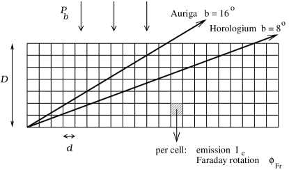
Figure 3: Depth depolarization model on a grid of thickness $D$, containing cells with cell size $d$. Synchrotron emission $I_{c}$ is emitted in each cell, Faraday rotation only occurs in a fraction $f$ of the cells. A constant background polarization $P_{b}$ is also Faraday-rotated while propagating through the medium. Along 2 lines of sight (Auriga and Horologium) the model is compared to observations.

We describe structure in the warm gas and in the magnetic field in the thin disk with a single-cell-size model. Fig. 3 gives a sketch of the model and its parameters; in addition to the cell size $d$ these are $D$, the vertical thickness of the layer, and the synchrotron emissivity $I_{c}$ in each cell. The warm ionized medium has a filling factor $f$; this is accounted for in the model by setting the electron density to an assumed constant value $n_{e}$ in a fraction $f$ of the cells along the line of sight, which are randomly chosen. In the remaining fraction $(1-f)$ of cells, $n_{e}$ is set to zero as an approximation for both the hot dilute gas and the cold neutral medium. Thus, we have made the simplifying assumption that neither the hot nor the cold gas contribute significantly to the $RM$.

The magnetic field in the thin turbulent disk consists of a random and a regular component $B_{ran}$ and $B_{reg}$. The field strengths of both components are assumed constant (but not equal). As it is not known how $B_{ran}$ and $B_{reg}$ in the cold, warm and hot phases of the ISM are related, we consider two extreme cases:

• properties of both the random and the regular component of the magnetic field are identical in all phases of the ISM.

• the random component of the magnetic field only exists in the turbulent warm ISM. In the cold and hot ISM, the regular magnetic field component predominates. The total magnetic field energy density is equal in all phases.

Hence, the properties of the cells are identical in both models – they contain $n_{e}$, $B_{ran}$ and $B_{reg}$. The difference between models A and B is the hot/cold medium (outside the cells) which contains $B_{ran}$ and $B_{reg}$ (model A), but only $B_{reg}$ in model B.

In each cell, an amount of synchrotron radiation $I_{c}\propto B_{\perp}^{2}$ is emitted, which is assumed to be 70% linearly polarized. In the cell, the polarized component of this emission and all emission from behind is Faraday rotated by an amount $\phi_{Fr}$.

The thick synchrotron disk serves as a background to the detailed model of the thin disk described here. We assume that the structure in the thick disk is on such large scales that we can approximate the background as a uniform synchrotron emitter, producing a constant polarized intensity $P_{b}$ as input to the thin disk, with uniform polarization angle. $P_{b}=0.7\;\eta_{b}\;I_{b}$, where $I_{b}$ is the total intensity of the background, and $\eta_{b}$ is a constant depolarization factor describing the depolarization due to the thick disk, with $0\leq\eta_{b}\leq 1$. Details of the emission and propagation of the radiation can be found in Appendix A.

Each line of sight through the model grid (to be identified with the direction of one of our fields, and corresponding to a particular Galactic latitude) is simulated many times, by independently filling the cells that contain the warm ISM, and by redrawing the angle that the random component of the magnetic field makes with the line of sight. An ensemble of such realizations, for which we derive the distributions of $I$, $Q$, $U$ and $RM$, simulates the many lines of sight for which we obtain the same information in one of the observed fields. So, only the statistical information of these distributions is included in the model, not the discrete structure. Each of the two observed regions separately already provides useful constraints for the model parameters (see below), but the combined set of constraints in Table 2 is quite powerful by virtue of the different path lengths through the medium.

As we model many lines of sight by redrawing the same line of sight many times for different models, beam depolarization is not included in the models.

5.2 The various types of model parameters

Four types of parameters, listed in Table 4, are used in the model. We discuss these separately.

Input parameters with fixed values

These are physical parameters which can be estimated or for which reasonably good estimates exist in the literature. From dispersion measures ($DM$) of pulsars in globular clusters at high Galactic latitude and H$\alpha$ emission measures ($EM$), Reynolds (1991) derives $n_{e}\approx$ 0.08 cm^-3, with a filling factor $f=$ 40% if the warm ionized ISM layer has a constant electron density, and 20% if the electron density distribution is exponential. The Beuermann et al. (1985) model for Galactic synchrotron radiation predicts a half equivalent width of the thin disk of 180 pc. We run the model with fixed values $f=$ 20%, $D=180$ pc and $n_{e}=$ 0.08 cm^-3 and discuss afterwards how the results would change if these parameters were different.

The intrinsic polarization angle of the background only defines the average angle in the final map of polarization angle. It changes the $Q$ and $U$ maps locally, but has no influence on the distributions of $Q$ and $U$. Therefore the value of $\phi_{0}$ is arbitrary and chosen to be 0${}^{\mbox{\tiny o}}$. The angles $\alpha$ and $\phi_{r}$ define the orientation of the random component of the magnetic field, with respect to the line of sight and some fixed direction in the plane of the sky, respectively. Both are randomly drawn from uniform distributions, for each cell.

The total intensity $I_{0}$ is taken from the 408 MHz all-sky survey by Haslam et al. (1982). The 2.7 K contribution from the CMBR is subtracted before these data are converted to a frequency of 350 MHz using a spectral index of –2.7. Approximately 25% of the total background temperature is due to point sources (from source counts, Bridle et al. 1972), so only the remaining 75% is included in the model. This yields values of 34 K and 47 K for $I_{0}$ in Auriga and Horologium, respectively.

The proportionality constant $C=1$ is estimated from the local cosmic ray spectrum, see Appendix B. If strict equipartition between cosmic rays and magnetic field applies, then $C$ is not constant but varies with $B_{\perp}^{2}$, so that the synchrotron emission $I\propto B_{\perp}^{4}$. Although equipartition is believed to hold on global Galactic scales, it is highly uncertain if equipartition is valid at parsec scales as well, because fluctuations in the supply rate of cosmic rays may destroy equipartition on small scales. Therefore, the exponent $\alpha$ of the relation $I\propto B_{\perp}^{\alpha}$ could be between 2 and 4. Although Burn (1966) concludes that equipartition does not influence the depolarization much, Sokoloff et al. (1998) find that in the case of equipartition the depolarization effects can differ by maximally 25%. We assume $\alpha=2$ in the model, and discuss afterwards the change in parameter values if $\alpha>2$.

Free input parameters

No external constraints are imposed on the cell size $d$. Estimates of cell sizes from the literature range from 10 pc to about 100 pc, and mostly probe scales that exceed the size of our fields. We probe cell sizes from a parsec to several tens of parsecs, and find the cell size determined in a reasonably narrow range because of the observational constraints.

Constraints determined from the observations

Parameter	Auriga region	Horologium region
$RM_{0}$	–3.4 rad m-2	–1.4 rad m-2
$\sigma_{\scriptscriptstyle\rm RM}$	1.8 rad m-2	4.3 rad m-2
$\sigma_{I}$	$\leq$ 1.7 K	$\leq$ 2.5 K
$\sigma_{Q,U}$	3 K	4.3 K
Additional constraints:
Distributions of $RM$, $I$, $Q$, and $U$ are Gaussian

Table 2: Values of observationally determined parameters from polarization maps of the Auriga and Horologium regions and other observational constraints for the models.

As discussed in Sect. 2, our observations yield distributions of $I$, $Q$, $U$ and $RM$. We summarize these results in Table 2, in the form of the mean value of observed $RM$, $RM_{0}$, and the dispersions $\sigma_{RM}$, $\sigma_{I}$, $\sigma_{Q}$ and $\sigma_{U}$. In the Auriga field, the dispersion in $RM$ was derived after subtraction of the best-fit gradient in $RM$ (see Sect. 2). Like in the observations, only reliably determined $RM$s are used.

Model parameters that can be adjusted and optimized

For any chosen value of cell size $d$, the model contains five parameters that are not derived from external data or from the observations. These are: the parallel and perpendicular components of the large-scale magnetic field, $B_{reg,\parallel}$ and $B_{reg,\perp}$ respectively, the strength of the random component of the magnetic field $B_{ran}$, the intensity of the polarized emission from the thick disk $P_{b}$, and the thick disk depolarization factor $\eta_{b}$ which connects $P_{b}$ and $I_{b}$. The five parameters have specific dependences on the observables, as is depicted in Table 3.

Parameter	depends on
$RM_{0}$	$B_{reg,\parallel}$
$\sigma_{\scriptscriptstyle\rm RM}$	$B_{reg,\parallel}$, $B_{ran}$
$\sigma_{I}$	$B_{ran}$, $B_{reg,\perp}$
$\sigma_{Q,U}$	$B_{ran}$, $B_{reg,\perp}$, $P_{b}$
$I_{0}$	$B_{ran}$, $B_{reg,\perp}$, $P_{b}$, $\eta_{b}$

Table 3: Observables and their dependencies

This makes it possible to determine definite values for most free parameters, e.g. $B_{reg,\parallel}$ can be determined because $RM_{0}$ only depends on $B_{reg,\parallel}$. The free parameters are determined as follows (where the subscript $obs$ means the observed value):

1. Set $B_{reg,\parallel}$ to obtain $RM_{0}=RM_{0,obs}$

2. Set $B_{ran}$ to obtain $\sigma_{\scriptscriptstyle\rm RM}$ = $\sigma_{\scriptscriptstyle\rm RM}$_,obs

3. Set $B_{reg_{\perp}}$ to match $\sigma_{I}=\sigma_{I,obs}$. Then:

   • If $\sigma_{Q,U}<\sigma_{Q,U,obs}$: set $P_{b}>0$ to obtain $\sigma_{Q,U}=\sigma_{Q,U,obs}$

   • If $\sigma_{Q,U}>\sigma_{Q,U,obs}$: decrease $B_{reg_{\perp}}$ and find a range of ($B_{reg_{\perp}}$, $P_{b}$) for which $\sigma_{I}<\sigma_{I,obs}$ and $\sigma_{Q,U}=\sigma_{Q,U,obs}$, with the additional constraint that the $Q$ and $U$ distributions remain Gaussian.

4. Set $\eta_{b}$ to obtain the correct value of $I_{0}$

Figure 4: Dependences of depth depolarization parameters on observables in the Auriga region, for model A. Left plot: $RM_{0}$ increases with $B_{reg,\parallel}$. Center plot: for fixed $B_{reg,\parallel}$, $\sigma_{\scriptscriptstyle\rm RM}$ increases with $B_{ran}$, with only a weak dependence on the value of $B_{reg,\parallel}$. Right plot: $\sigma_{Q,U}$ depends on $B_{ran}$ and $B_{reg,\perp}$.

An example of the correlations used is given in Fig. 4. The leftmost plot shows the dependence of $RM_{0}$ on $B_{reg,\parallel}$. As expected, a large regular magnetic field component causes a large non-zero mean RM (the negative value of the magnetic field reflects the observed negative $RM_{0}$). The center plot gives the change of $\sigma_{\scriptscriptstyle\rm RM}$ with $B_{ran}$ for three fixed values of $B_{reg,\parallel}$, which increases roughly linearly with $B_{ran}$ and shows hardly any dependence of $\sigma_{\scriptscriptstyle\rm RM}$ on $B_{reg,\parallel}$. Having set $B_{ran}$ to obtain the observed value of $\sigma_{\scriptscriptstyle\rm RM}$  the right plot shows how the observable $\sigma_{Q,U}$ depends on $B_{reg,\perp}$. The width of the $Q$ and $U$ distribution depends slightly on the chosen values of $B_{ran}$.

6 Results from the model

For models A and B as defined in Sect. 5.1, the propagation of polarized radiation through the medium is computed for a range of values of the cell size $d$, which results in values for the five adjustable parameters for each $d$.

The allowed cell size is well-constrained by the observations: if the cell size is large, the number of cells is small for a given path length and filling factor. As the number of cells with Faraday-rotating, thermal medium can differ per line of sight, the $RM$ distribution will not be Gaussian anymore if the cells are chosen too large. On the other hand, if the cell size is small, the $RM$ per cell decreases. But to obtain a large enough $\sigma_{\scriptscriptstyle\rm RM}$, the $RM$ per cell has to be rather high, so the parameter $B_{ran}$ has to be increased to produce the observed value of $\sigma_{\scriptscriptstyle\rm RM}$. However, an increase of $B_{ran}$ increases $\sigma_{I}$, which then puts an upper limit on $B_{reg,\perp}$. To produce the observed dispersion in $Q$ and $U$, we then need a large value for the background polarized intensity $P_{b}$. If the cell size is taken too small, $P_{b}$ becomes so large compared to the polarized emission in the cells, that the distributions of $Q$ and $U$ become distinctly non-Gaussian. Allowed values of $d$ range from approximately 1 to 60 pc, with an optimum value of about 15 pc, in good agreement with estimates by Ohno & Shibata (1993). However, a cell size of 15 pc located at the far end of the thin disk in the direction of the Auriga region subtends an angle of more than a degree on the sky. As we observe structure on degree to arcminute scales, smaller cells must be present as well. Most likely, a power law spectrum of turbulence is present on these scales (Clegg et al. 1992, Armstrong et al. 1995, Minter & Spangler 1996). An extension of the model including a power law spectrum of cell sizes would increase the depolarization along the line of sight, thereby decreasing the random magnetic field strength needed.

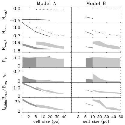
Figure 5: Allowed ranges of parameters for model A (left) and B (right) for different values of cell sizes. The magnetic field values are given in $\mu$G, the polarized brightness temperature of the background $P_{b}$ in K and $I_{0,thin}$ is the percentage of the total emissivity that originates in the thin disk. The lines in the upper plots show values found for $B_{reg,\parallel}$ and $B_{ran}$ for the Auriga region (solid line) and the Horologium region (dotted line). All plots below those show allowed ranges in parameters for the Auriga region (dark) and Horologium (light).

We now summarize the result of the comparison between the models and the observations. The cell sizes probed in the modeling were 1, 2, 5, 10, 20, 30, 40 and 60 pc, although for model B, only cell sizes above 5 pc are allowed, and smaller cell sizes are allowed for the Auriga region than for Horologium.

Fig. 5 shows the allowed ranges of parameters in the two regions for models A (left) and B (right). The upper plots show values of the obtained parallel regular field $B_{reg,\parallel}$, where the solid line denotes Auriga and the dotted line Horologium. $B_{reg,\parallel}$ is $-0.42\pm 0.02\leavevmode\nobreak\ \mu$G for Auriga and $-0.085\pm 0.005\leavevmode\nobreak\ \mu$G for Horologium in model A, and $-0.35\pm 0.01$ $\mu$G and $-0.065\pm 0.005\leavevmode\nobreak\ \mu$G respectively in model B, where the errors are estimated from the spread in observed values. $B_{reg,\parallel}$ hardly depends on cell size. The next plots down show $B_{ran}$, where the best value is about 1 $\mu$G for large ($\ga 5$ pc) cell sizes for both the Auriga and the Horologium region, and increases to $\sim\leavevmode\nobreak\ 4\leavevmode\nobreak\ \mu$G for cell sizes of a parsec.

For the remaining parameters $B_{reg,\perp}$, $P_{b}$, and $\eta_{b}$ only parameter ranges could be determined instead of definite values, given in Fig. 5 by a dark grey region for Auriga and light grey for Horologium. The edges of the shaded areas are not sharp as drawn but have a considerable uncertainty. The allowed parameter range should be read more as an indication of possible parameter values than as ranges with sharp boundaries. Moreover, the discrete edges at a certain cell size only indicate that the next probed cell size could not produce parameters in agreement with the observations.

The perpendicular component of the regular magnetic field $B_{reg,\perp}$ is approximately $2.8\pm 0.5\leavevmode\nobreak\ \mu$G in Auriga and $3.2\pm 0.5\leavevmode\nobreak\ \mu$G in Horologium for both models. The intensity of the polarized background $P_{b}$ varies between 0.1 and 3 K, with a best estimate of about 1.5 $\pm$ 1.0 K. The depolarization factor $\eta_{b}=P_{b}/(0.7I_{b})$ of the thick disk ranges from almost zero to 0.6 with a best estimate of about 0.15 $\pm$ 0.1.

Below that, $B_{ran}/B_{reg}$ is given, which varies between 0.5 and 1.5 but is mostly smaller than one. The bottom plots show $I_{0,thin}$, the percentage of the total synchrotron emission generated in the thin disk, to be between 20% and 75%, and decreasing for larger cell sizes.

Having determined these parameter ranges, we vary the filling factor $f$, thermal electron density $n_{e}$ or thickness $D$ while keeping all earlier determined parameters fixed, to gauge their influence on the model output parameters. A filling factor $f\la$ 5 – 10% is not allowed in either model: large cell sizes give a non-Gaussian $RM$ distribution, and small cell sizes yield too high a background polarization to keep $Q$ and $U$ Gaussian. No upper limit can be given for the filling factor, and $B_{ran}/B_{reg}$ decreases with a factor two for $f=1$. For varying thermal electron density, a low $n_{e}$ $\la 0.03$ cm^-3 dictates such a high $B_{ran}$ that the ratio $B_{reg,\perp}/P_{b}$ becomes so low that $Q$ and $U$ become distinctly non-Gaussian. High electron densities are allowed in the models but the random magnetic field drops to very low values ($B_{ran}\la 0.15\leavevmode\nobreak\ \mu$G for $n_{e}\ga 0.1$ cm^-3). A lower limit to the thickness of the thin disk is about 100 pc, again no upper limit can be set. The difference between a thickness of 150 pc or 180 pc is negligible.

We checked the influence of the assumption of equipartition between magnetic field and cosmic rays. If $I\propto B_{\perp}^{4}$ instead of $I\propto B_{\perp}^{2}$, the upper limit to structure in $I$ becomes much more stringent. Therefore, model A will no longer produce any solutions that agree with the observables. In model B solutions are found with cell sizes 10 and 20 pc, and $B_{reg,\perp}$ much lower, about 0.5 $\mu$G. Other parameters are comparable to the case where $I\propto B_{\perp}^{2}$.

Finally, it should be mentioned that the mean values of the distributions of $Q$ and $U$, which are large-scale components that are not observable with an interferometer, are lower than 1.2 K in all models for all parameters. These large-scale components are negligibly small, in agreement with Haverkorn et al. (2004).

6.1 Discussion of the resulting model parameters

A basic first conclusion is that the values obtained in the two regions roughly agree, even though the Auriga and Horologium regions have different input parameters and a different line of sight through the medium. The regular magnetic field components approximately agree in the two regions ($B_{reg}\approx 3\leavevmode\nobreak\ \mu$G).

From the deduced depolarization factor $\eta_{b}=0.15$, we can estimate the halo magnetic field, assuming a constant background. Around 350 MHz, depth depolarization of a uniform medium to 0.15 times the original polarization is caused by $RM$ $\approx 3-5$ rad m^-2 (Burn 1966), which indicates a value of $B_{\parallel}\approx 0.1\mu$G for a height of the Reynolds layer of 1 kpc and $n_{e}\approx 0.05$ cm^-3 in the halo. So the disk magnetic field could persist with only slight attenuation throughout the Reynolds layer, as was suggested earlier by Han et al. (1999).

Our estimate of $B_{ran}/B_{reg}<1$ is somewhat lower than most of the estimates from the literature discussed in Section 4. This may be due to several factors. First, random magnetic field structure on scales larger than our field of view ($\sim 7\mbox{${}^{\mbox{\tiny o}}$}\times 9\mbox{${}^{\mbox{\tiny o}}$}$) will be interpreted as regular field in our analysis. Secondly, it could be the result of selection, as our observational fields were chosen for their high polarized intensity, which in our model automatically implies a modest random magnetic field. Finally, the observations are in the second Galactic quadrant, so we probe mostly the inter-arm region between the Local and the Perseus arms, where $B_{ran}/B_{reg}$ is smaller than in the average ISM including spiral arms (e.g. Indrani and Deshpande 1998, Beck 2001).

The emission in the thin disk $I_{0,thin}$ is also estimated by Beuermann et al. (1985) in their standard decomposition of $I_{0}$ into thin and thick disk contributions. According to their model, only about 20 to at most 35% of $I_{0}$ is generated in the thin disk and the nearest 180 pc of the thick disk. Furthermore, Caswell (1976) estimated the synchrotron emissivity from a survey with the Penticton 10 MHz array as 240 K pc^-1 at 10 MHz. Rescaled to 350 MHz, this gives a total emission from the thin disk of 10.6 K in the Auriga region and 21 K in the Horologium region. Roger et al. (1999) estimate from the 22 MHz survey performed with the DRAO 22 MHz radio telescope an emissivity of about 55 K pc^-1 for two HII regions in the outer Galaxy, out of the Galactic plane. Their results give estimates of the emissivity in the thin disk which are approximately twice as high as the estimates from the Caswell survey. Due to the large uncertainty in the emissivity, $I_{0,thin}$ does not put a strong constraint on the model parameters.

6.2 A “polarization horizon”?

Figure 6: Observed fraction of polarization originating closer than a certain distance against the path length, for the Auriga region (solid line) and the Horologium region (dashed line).

A “polarization horizon” is defined as a distance beyond which (most of the) emitted polarized emission is depolarized when it reaches the observer (Landecker et al. 2001). This can be due to beam depolarization, when the angular scale of the structure in the polarized emission becomes smaller than the synthesized beam at a certain distance. If the smallest scales in the observed regions are about a parsec, the angle of these scales on the sky becomes smaller than the beam at a distance of about 700 pc. Spoelstra (1984) derived the polarization horizon from comparison of radio continuum data at five frequencies from 408 MHz to 1411 MHz (Brouw & Spoelstra 1976) with starlight polarization. He found a distance to the origin of the polarized radio emission of 625 $\pm$ 125 pc in the direction of our fields.

Furthermore, the resulting degree of polarization decreases for increasing pathlength through a rotating and emitting medium. However, as depolarization is a process occurring in a telescope and not in the medium itself, it cannot be determined what distance the remaining polarized radiation originated. We can only estimate the decrease in polarization as a function of path length. In our model, we build up a line of sight by adding cells one by one, starting at the observer. The radiation from each added cell is Faraday-rotated by all warm ionized material in front of it. The observed degree of polarization after addition of each cell is given as a function of the line of sight built up until that particular cell in Fig. 6, for the Auriga (solid line) and Horologium (dashed line) regions, for model A with a cell size of 5 pc. Even for the total path length through the thin disk, still a fairly large fraction (20%) of the polarized emission can be observed. Therefore, depth depolarization alone cannot produce a true horizon, but attenuates the polarization gradually with path length.

From both arguments, we estimate a distance of about 600 to 700 pc as the critical path length (“polarization horizon”). Polarized radiation traveling along significantly larger path lengths than this is expected to be largely depolarized.

7 Summary and conclusions

Depth depolarization, the depolarization process along the line of sight in a medium of synchrotron-emitting and Faraday-rotating material, is the dominant cause of structure in polarized intensity which is unrelated to total intensity fluctuations.

We modeled the effect of depth depolarization with a simple model of the Galactic ISM consisting of a layer of cells containing random and regular magnetic field $B_{ran}$ and $B_{reg}$, and thermal electron density $n_{e}$ in a fraction $f$ of the cells (mimicking the filling factor $f$). This layer corresponds to the Galactic thin disk with small-scale structure in the magnetic field. The Galactic thick disk or halo is modeled by a constant background $P_{b}$, with a certain constant depolarization denoted by the factor $\eta_{b}$. We vary cell size, magnetic field and background to obtain a range of models that comply to the observational constraints, i.e. yield the correct width, mean and shape of the distributions of $Q$, $U$ , $I$ and $RM$.

The results can be summarized as follows: the allowed cell size is constrained to be in the range of 1 to 60 pc, with a best estimate of 15 pc. The regular magnetic field component along the line of sight ($\sim-0.4\leavevmode\nobreak\ \mu$G for Auriga, and $\sim-0.08\leavevmode\nobreak\ \mu$G for Horologium) is much smaller than the regular magnetic field component perpendicular to the line of sight ($\sim 2.8\leavevmode\nobreak\ \mu$G for Auriga, and $\sim 3.2\leavevmode\nobreak\ \mu$G for Horologium), indicating that the regular magnetic field is directed almost perpendicular to the line of sight in these directions. The random magnetic field component is about 1 to 3 $\mu$G in the two regions. In most of our models, the regular component of the magnetic field was found to be higher than the random component, with an average ratio of $B_{ran}/B_{reg}=0.7\pm 0.5$ which increases for smaller cell sizes. Estimates from the literature tend to give larger ratios (0.5 – 4). This could be explained by the size of our fields of view ($\sim$ 7${}^{\mbox{\tiny o}}$ in size), so that random components of the magnetic field on scales large than the field are misinterpreted as regular components. Furthermore, the fields of observation were selected for their high polarization, indicating a higher regular magnetic field component than average, and are situated in an inter-arm region, where uniform magnetic fields tend to be higher than average. The constant polarized background intensity from the thick disk is about $1.5\pm 1.0$ K.

This model forms a promising first attempt to derive properties of the Galactic magnetic field from observed polarization and rotation measures. In future work, the model can be expanded e.g. using a power law distribution of the structure. Furthermore, cell size, filling factor and electron density appear to be correlated (Berkhuijsen 1999), which should be incorporated in a future version. New observations in different directions can narrow down the parameter space considerably.

Appendix A Outline of the depth depolarization model

Input parameters with fixed values		value:
$n_{e}$	thermal electron density in cells	0.08 cm-3 (Reynolds 1991)
$f$	filling factor of the warm ISM	20% (Reynolds 1991)
$D$	thickness of the layer with cells	180 pc (Beuermann et al. 1985)
$\phi_{0}$	intrinsic polarization angle of the background	arbitrary: 0${}^{\mbox{\tiny o}}$ chosen
$\phi_{r}$	position angle of random magnetic field	random per cell
$\alpha$	angle between random magnetic field and line of sight	random per cell
$I_{0}$	total intensity	Auriga: 34 K
		Horologium: 47 K (from Haslam et al. 1982)
$C$	proportionality constant between $I_{c}$ and $B_{\perp}^{2}$	$C=1$, see Appendix B
Free input parameters
$d$	cell size
Constraints determined from the observations
$RM_{0}$	mean rotation measure
$\sigma_{\scriptscriptstyle\rm RM}$	width of $RM$ distribution
$\sigma_{I}$	width of $I$ distribution
$\sigma_{Q,U}$	width of $Q$, $U$ distribution
Model parameters that can be adjusted and optimized		set by dependence of:
$B_{reg,\parallel}$	parallel component of regular magnetic field	$RM_{0}$ ($B_{reg,\parallel}$)
$B_{ran}$	(constant) strength of random magnetic field	$\sigma_{\scriptscriptstyle\rm RM}$ ($B_{reg,\parallel}$,$B_{ran}$)
$B_{reg,\perp}$	perpendicular component of regular magnetic field	$\sigma_{I}$ ($B_{ran}$,$B_{reg,\perp}$)
$P_{b}$	polarized intensity of background	$\sigma_{Q,U}$ ($B_{ran}$,$B_{reg,\perp}$,$P_{b}$)
$\eta_{b}$	factor for depolarization of background	$I_{0}$ ($B_{ran}$,$B_{reg,\perp}$,$P_{b}$,$\eta_{b}$)
Additional constraints:
background depolarization factor $0\leq\eta_{b}\leq 1$
Number of cells $N=L/d$, while $Nf$ cells determine the shape of $RM$ distribution
$B_{reg,\perp}$/$P_{b}$ determines shape of $Q$, $U$ distribution

Table 4: The first set of parameters is determined from the literature or can be arbitrarily chosen. The second set is varied in the models, and the third set of parameters is set by our observations. The last set are those parameters of the ISM that can be estimated from the models, followed by the input parameters from the categories above. In parentheses the model parameters that they depend on.

The synchrotron radiation emitted in each cell is $I_{c}\propto B_{\perp}^{2}$. This emission, and the emission from each cell further away along the line of sight and from the background passing through the cell, is Faraday rotated by an amount $\phi_{Fr}$. So in each cell:

$$I_{c} = \frac{C}{N}\;\left[(B_{ran}\sin\alpha)^{2}+B_{reg,\perp}^{2}\right]$$ (1)

$$\phi_{Fr} = RM\lambda^{2}=0.81\;n_{e}\;(B_{ran}\cos\alpha+B_{reg,\parallel})\;d\lambda^{2}$$

$$P_{c} = 0.7\;I_{c}$$

where $B_{ran}$ is the constant strength of the random magnetic field in $\mu$G, $\alpha$ its random angle with the line of sight, $C$ a proportionality constant, $N$ the number of cells along the line of sight and $d$ the path length. The total emission from the layer ($\approx CN$) is comparable for different cell sizes, therefore a factor $1/N$ is added to Eq. (1). The polarized emission in each cell $P_{c}$ equals the maximum polarization of synchrotron radiation $I_{c}$ generated in a cell. For an electron energy power law distribution $N(E)\propto E^{-\gamma}$, the degree of polarization $p$ is related to the spectral index $\gamma$ of the electron energy distribution as $p(\gamma)=(3\gamma+3)/(3\gamma+7)$ (Burn 1966). For $\gamma$ around 2.7, the maximum polarization is $\sim$ 70% of the total intensity. The polarization angle of the emission generated in each cell $\phi_{in}$ is taken to be perpendicular to the position angle of the perpendicular magnetic field. The position angle of the random magnetic field component $\phi_{r}$ is random, and that for the regular component is chosen in the direction of Galactic longitude. Therefore the polarized intensity emerging from a cell is

$${\mathbf{P}_{c}}=0.7I_{c}\;{\rm e}^{-2i(\phi_{Fr}+\phi_{in})}+0.7I_{b}\;{\rm e}^{-2i(\phi_{Fr}+\phi_{b})}$$ (2)

for a cell that is irradiated with polarized intensity $I_{b}$ and polarization angle $\phi_{b}$. The input and output parameters are given in Table 4.

Appendix B Estimate of the parameter $C$

The total power per unit volume per unit frequency of synchrotron emission is (Rybicki & Lightman 1979)

$$P_{tot}(\omega) = \frac{\sqrt{3}q^{3}\kappa^{\prime}B\sin\alpha}{2\pi mc^{2}(p+1)}\,\Gamma\left(\frac{p}{4}+\frac{19}{12}\right)\Gamma\left(\frac{p}{4}-\frac{1}{12}\right)$$ (3)

$$\times\left(\frac{mc\omega}{3qB\sin\alpha}\right)^{-(p-1)/2}$$

$$= \frac{3\sqrt{3}}{16\pi^{2}}\frac{q^{4}\kappa^{\prime}B_{\perp}^{2}}{m^{2}c^{3}\nu}\Gamma\left(\frac{28}{12}\right)\Gamma\left(\frac{2}{3}\right)\,\,\,\mbox{for $p=3$}$$

where $q$ is the electron charge, $\kappa^{\prime}$ is the proportionality constant in a power law particle spectrum $N(\gamma)$ with spectral index $p$ ($N(\gamma)d\gamma=\kappa^{\prime}\gamma^{-p}d\gamma$), $B\sin\alpha=B_{\perp}$ is the magnetic field component perpendicular to line of sight, $m$ is the electron mass, $c$ the speed of light and $\omega$ the angular frequency of the radiation. $\Gamma$ denotes the gamma-function.

We can estimate $\kappa^{\prime}$ by assuming that the electron particle spectrum throughout the ISM is equal to the local value in the solar neighborhood. Longair (1981) gives a value of $\kappa=2.9\leavevmode\nobreak\ 10^{-5}$ particles m^-3 GeV^-(1-p) for the proportionality constant of the particle spectrum as a function of energy $N(E)dE=\kappa E^{-p}dE$ derived from direct measurements of the particle spectrum in the local ISM, in agreement with the value found by Golden et al. (1994). This can be converted into $\kappa^{\prime}$ as $\kappa^{\prime}=\kappa(mc^{2})^{(1-p)}$. Using $p=3$ and converting to cgs units gives $\kappa^{\prime}=1.0\leavevmode\nobreak\ 10^{-4}$ part cm^-3 ergs². Inserting this into Eq. (3) yields

$$P_{tot}(\nu)=4.2\leavevmode\nobreak\ 10^{-39}\frac{B_{\perp}[\mu\mbox{G}]^{2}}{\nu[\mbox{MHz}]}\mbox{\leavevmode\nobreak\ W\leavevmode\nobreak\ m${}^{-3}$\leavevmode\nobreak\ Hz${}^{-1}$}$$ (4)

This is the volume emissivity of synchrotron emission as a function of frequency and magnetic field. We can check how reasonable this number is by comparing to the total power observed from the Caswell (1976) radio survey at 10 MHz. The average brightness temperature computed by Caswell corresponds to a volume emissivity of $\sim 3\leavevmode\nobreak\ 10^{-39}$ W m^-3 Hz^-1 (Longair 1981), which agrees well with our value of $P_{tot}(10\leavevmode\nobreak\ \mbox{MHz})=0.42\leavevmode\nobreak\ 10^{-39}\leavevmode\nobreak\ B_{\perp}[\mu\mbox{G}]^{2}$ W m^-3 Hz^-1 for $B_{\perp}=3\leavevmode\nobreak\ \mu$G.

The next step is to describe $P_{tot}$ in terms of the observables. The observables are in Kelvin, whereas $P_{tot}$ is in W m^-3 Hz^-1. The power that is detected on 1 m² of antenna surface is

$$P_{cell,ant}\leavevmode\nobreak\ [\mbox{W\leavevmode\nobreak\ Hz${}^{-1}$\leavevmode\nobreak\ m${}^{-2}$}]=\frac{d^{3}}{4\pi D^{2}}P_{tot}\leavevmode\nobreak\ [\mbox{W\leavevmode\nobreak\ m${}^{-3}$\leavevmode\nobreak\ Hz${}^{-1}$}]\\$$

with $D$ the distance to the cell. This gives the emissivity of a source in the direction of the observer on 1 m² of dish in Jansky’s. Then, to convert into Jansky/beam, only consider the part of the source which fits into a beam. With a spatial resolution of $D\tan(5^{\prime})$, the area of a beam is $\pi(1/2\leavevmode\nobreak\ D\tan(5^{\prime})^{2})$, and the number of beams that fits into the source is $4d^{2}/(\pi D^{2}\tan^{2}(5^{\prime}))$. Then the emissivity in one cell per beam is

$$I_{c}[\mbox{W\leavevmode\nobreak\ Hz${}^{-1}$\leavevmode\nobreak\ m${}^{-2}$\leavevmode\nobreak\ beam${}^{-1}$}]\;=\;\hskip 113.81102pt$$

$$\frac{d^{3}}{4\pi D^{2}}\left(\frac{\pi D^{2}\tan^{2}(5^{\prime})}{4d^{2}}\right)P_{tot}\leavevmode\nobreak\ [\mbox{W\leavevmode\nobreak\ m${}^{-3}$\leavevmode\nobreak\ Hz${}^{-1}$}]$$

so that, using Eq. (4), the emissivity $I_{c}$ in Jy/beam is $I_{c}=0.21\;d$[pc] K using that 1 mJy/beam $\approx$ 0.13 K at 350 MHz. Combining this result with Eq. (1) yields an estimate for $C$:

$$C=\frac{0.21L}{\nu}\approx 0.5$$

for a path length L = 900 pc and $\nu=350$ MHz, where we used $N=L/d$. We use a value of $C=1$ in the model.