QSO size ratios from multiband monitoring of a microlensing high–magnification event

We introduce a new scheme to study the nature of the central engine in a lensed QSO. The compact emission regions could have different sizes in different optical wavelengths, and our framework permits to obtain the source size ratios when a microlensing special high–magnification event (e.g., a caustic crossing event, a two–dimensional maximum crossing event and so on) is produced in one of the QSO components. To infer the source size ratios, only cross–correlations between the brightness records in different optical bands are required. While the deconvolution method leads to a richer information (1D intrinsic luminosity profiles), the new approach is free of the technical problems with complex inversion procedures. Using simulations related to recent $VR$ data of Q2237+0305A, we discuss the ability of the scheme in the determination of the visible–to–red ratio $q=R_{V}/R_{R}$. We conclude that extremely accurate fluxes (with a few $\mu$Jy uncertainties, or equivalently, a few milli–magnitudes errors) can lead to $\sim$ 10% measurements of $q$. Taking into account the errors in the fluxes of Q2237+0305A from a normal ground–based telescope, $\sim$ 10 $\mu$Jy ($\sim$ 10 mmag), it must be possible the achievement of smaller errors from the current superb–telescopes, and thus, an accurate determination of $q$. Obviously, to measure the visible–to–red ratio, the light curves cannot be contaminated by an intrinsic event or an important high–frequency intrinsic signal, i.e., exceeding the $\mu$Jy (mmag) level. For an arbitrary lensed QSO, we finally remark that the framework seems to work better with very fast microlensing events.

1 Introduction

In an optical component of a lensed quasar, we might see large flux variations as a result of gravitational microlensing. Some high–magnification events (HMEs) occur when the compact source crosses fold caustics. In caustic crossing events (CCEs), the folds are assumed to be straight lines, or more properly, the source radius and the source path are assumed to be small compared to the caustic curvature radius. This approach is realistic for short trajectories of sufficiently compact sources. However, for long paths in parallel to fold caustics or broad–line regions crossing folds, the curvature effects can be important (e.g., Fluke & Webster 1999). We also note that the actual magnification maps contain assorted caustics, so the curvature radii of the smallest folds are probably equal or less than the source radius, and obviously, our approach is not valid in this ”dwarf” caustic case. The CCEs are prominent variations belonging to a wider family of special high-magnification events (SHMEs). The SHMEs are related to high–magnification regions in which the non–uniform amplification law, $A(X,Y)$, verifies that $A(kX,kY)=f(k)A(X,Y)$, with $k$,$f(k)>$ 0.

Grieger, Kayser & Refsdal (1988) suggested one important test on the nature of the compact source, which is based on the analysis of the observed light curve during an individual CCE. They showed that the one–dimensional intrinsic luminosity profile can be retrieved from the brightness record of a CCE. Other physical quantities can also be determined from observed CCEs (Grieger et al. 1988), but at present, it is not possible to fulfil all the observational requirements. In the nineties, the Grieger et al.’s original idea (deconvolution of the one–dimensional profile from an observed CCE) was developed by Grieger, Kayser & Schramm (1991), Agol & Krolik (1999), and Mineshige & Yonehara (1999), and currently, there are projects to apply it.

This paper deals with a different realistic test on the compact source structure: from the multiband monitoring of an individual SHME, one may measure the source size ratios, which inform about the nature of the emitter. In the past, some authors have also done multiband studies of quasar microlensing (e.g., Rauch & Blandford 1991; Wambsganss & Paczyński 1991; Jaroszyński et al. 1992; Yonehara et al. 1998; Yonehara el al. 1999). Here, we introduce a novel methodology to determine source size ratios in a direct and model–independent way. A hypothetical $UBVRI$ monitoring could lead to a very complete set of ratios, e.g., $R_{U}/R_{B}$, $R_{B}/R_{V}$, $R_{V}/R_{R}$ and $R_{R}/R_{I}$, while records in only two optical bands may be used to infer one ratio. From observed events in QSO 2237+0305 that were associated with CCEs (i.e., a kind of SHMEs), previous works discussed the size of the $VR$ sources (e.g., Wyithe et al. 2000; Shalyapin 2001; Yonehara 2001, Shalyapin et al. 2002), so indirect and model–dependent estimates of $q=R_{V}/R_{R}$ are available for that quasar. Shalyapin et al. (2002) reported indirect measurements of $q$ for several circularly symmetric source models, but unfortunately, the constraints on $q$ are usually weak (with large uncertainties) and depend on the assumed source model. If we only consider the results corresponding to the best source models (power–law with the smallest power index and accretion disk by Shakura & Sunyaev 1973), then it is derived a global interval 0.41 $\leq q\leq$ 1.26 (using 1$\sigma$ confidence limits). Therefore, for QSO 2237+0305 and other lensed quasars, we need a new tool to obtain an accurate and robust estimation of $q$ or another different ratio.

In Section 2 we present the new test. The method is robust, since it works with an arbitrary source model. Only similarity between the compact sources (corresponding to different optical filters) is required. More properly, the two–dimensional intensity distribution is arbitrary, but as usual, it is stationary. Therefore, while several popular scenarios are included in the methodology, e.g., a face–on standard disk or an inclined standard disk, we cannot discuss some scenarios, e.g., unstable or anisotropic (rotating) disks. In order to apply the test, we must focus on an observed SHME. Our method is only valid for the standard magnification close to a fold caustic and some non–standard amplification laws. In Section 2 we comment on a few non–standard behaviours leading to SHMEs. The techniques for obtaining the best value of $q$ as well as the criteria to measure the visible–to–red ratio are introduced in Section 3. Several details of the techniques are cumbersome and they are described in Appendix A. In Section 3, we also use synthetic light curves to test the power of the framework. The synthetic records are not arbitrary ones, but records related to the $V$–band and $R$–band GLITP (Gravitational Lensing International Time Project) microlensing peaks in the flux of Q2237+0305A (Alcalde et al. 2002; see also the corresponding OGLE event in Woźniak et al. 2000). Finally, in Section 4 we summarize and discuss our results.

2 The method: basic ideas

We concentrate on a component of a multiple (gravitationally lensed) quasar. In a given optical band, if the mass of the lens galaxy is mainly due to main sequence stars, white dwarfs, black holes and so on, gravitational microlensing high–magnification fluctuations are expected at different epochs. The compact source travels a magnification map in the source plane, which contains a caustic network with folds and cusps (e.g., Schneider, Ehlers & Falco 1992). In a high–magnification region, the radiation flux of the QSO component has two contributions: (a) a constant term ($F_{0}$) due to the extended source and a possible uniform magnification of the compact source, and (b) a variable contribution caused by the non–uniform magnification of the compact source, which is responsible for a prominent event.

We take two Cartesian coordinate frames: first, a source frame ($x$,$y$) in which the origin coincides with the compact source peak (the point with maximum intensity). The surface brightness distribution of the compact source is traced by the law $I(x,y)=I_{0}B(x/R,y/R)$, where $B$ is an arbitrary function that verifies $B(0,0)=1$ and $0\leq B<1$ at ($x$,$y$) $\neq$ (0,0), $R$ is the characteristic length of the intensity distribution and $I_{0}$ is the maximum intensity. Second, a magnification frame ($X$,$Y$), so the non–uniform magnification is $A(X,Y)$. At $t=t_{0}$, the magnification pattern frame coincides with the source frame. However, the origin of the magnification frame and the high–magnification region as a whole have an effective transverse motion, and we can split up the effective velocity in two parts: the motion parallel to the $x$-axis, $V_{\parallel}$, and the motion perpendicular to that axis, $V_{\perp}$. The random stellar motions in the lens galaxy are implicitly neglected during the high–magnification event. At a time $t$, the global flux is given by

$$F(t)=F_{0}+\frac{\epsilon I_{0}}{D_{s}^{2}}\int\int A[x-V_{\parallel}(t-t_{0}),y-V_{\perp}(t-t_{0})]B(x/R,y/R)dxdy,$$ (1)

where $\epsilon$ is the dust extinction factor, which ranges from 0 (complete extinction) to 1 (no extinction), and $D_{s}$ is the angular diameter distance to the source. Using normalized coordinates $\xi=x/R$ and $\eta=y/R$, one finds

$$F(t)=F_{0}+\frac{\epsilon I_{0}R^{2}}{D_{s}^{2}}\int\int A\{R[\xi-V_{\parallel}(t-t_{0})/R],R[\eta-V_{\perp}(t-t_{0})/R]\}B(\xi,\eta)d\xi d\eta.$$ (2)

On the other hand, we adopt a magnification law that is characterized by the property

$$A(kX,kY)=f(k)A(X,Y),$$ (3)

where $k$ is an arbitrary positive constant and $f(k)$ is another positive constant related to $k$. From Eqs. (2–3), a flux of the QSO component is inferred

$$F(t)=F_{0}+\frac{\epsilon I_{0}R^{2}f(R)}{D_{s}^{2}}J\left[\frac{V_{\parallel}(t-t_{0})}{R},\frac{V_{\perp}(t-t_{0})}{R}\right].$$ (4)

The $J$ function is given by $J[\tau,\omega]=\int\int A(\xi-\tau,\eta-\omega)B(\xi,\eta)d\xi d\eta$.

We remark two important issues. The first point deals with the high–magnification regions that are consistent with the property (3), and consequently, are related to SHMEs. The magnification law near a cusp caustic does not verify Eq. (3) (e.g., Schneider & Weiss 1992; Zakharov 1995). However, in the surroundings of a fold caustic, the behaviour of the non–uniform amplification is $A(X,Y)=a_{C}H(X)/\sqrt{X}$. Here, $H(X)$ is the Heaviside step function (e.g., Chang & Refsdal 1979; Schneider & Weiss 1987). It is evident that the previous standard amplification verifies Eq. (3), so the CCEs are included in our framework. Other non–uniform laws also agree with that equation. For example, the non–uniform magnifications around an one–dimensional maximum ($\alpha X^{2}$) and a two–dimensional maximum ($\alpha X^{2}+\beta XY+\gamma Y^{2}$) are characterized by $f(k)=k^{2}$. The relation between the non–standard behaviours and real regions in magnification patterns merits more attention. The source model is another important issue. With respect to this topic, we note that the two–dimensional intensity distribution can have circular symmetry, elliptical symmetry or a more complex structure, but it cannot evolve with time.

We consider a set of compact sources that are associated with a set of optical filters, so all sources have the same shape and peak. They only differ in their lengths and peak intensities. Although this hypothesis of similarity is useful to link different sources corresponding to different filters, it could be false in a real situation. However, the similarity between sources is consistent with the standard face–on accretion disk (e.g., Shalyapin et al. 2002; Kochanek 2004). During a SHME, in a first optical band (number 1), the theoretical light curve depends on the background flux $F_{01}$, the dust extinction $\epsilon_{1}$, the maximum intensity $I_{01}$ and the length $R_{1}$ (see Eq. 4). In a similar way, in a second optical band (number 2), one has the parameters $F_{02}$, $\epsilon_{2}$, $I_{02}$ and $R_{2}$. We can directly compare the flux in the 1-band at the time $t$ with the flux in the 2-band at the time $t^{\prime}$, when both times are linked from the relationship

$$\frac{t-t_{0}}{R_{1}}=\frac{t^{\prime}-t_{0}}{R_{2}}.$$ (5)

Alternatively, Eq. (5) can be rewritten as

$$t^{\prime}=r_{21}t+(1-r_{21})t_{0},$$ (6)

where $r_{21}=R_{2}/R_{1}$ is the source size ratio, and $t^{\prime}$ is obtained through a dilation ($r_{21}t$) and a delay ($t_{0}-r_{21}t_{0}$). At the time $t^{\prime}$, the 2-band flux fulfils

$$\frac{D_{s}^{2}\left[F_{2}(t^{\prime})-F_{02}\right]}{\epsilon_{2}I_{02}R_{2}^{2}f(R_{2})}=J\left[\frac{V_{\parallel}(t-t_{0})}{R_{1}},\frac{V_{\perp}(t-t_{0})}{R_{1}}\right],$$ (7)

so

$$F_{1}(t)=a+bF_{2}(t^{\prime}).$$ (8)

The constants $a$ and $b$ are given by $a=F_{01}-F_{02}b$ and $b=\left[\epsilon_{1}I_{01}R_{1}^{2}f(R_{1})\right]/\left[\epsilon_{2}I_{02}R_{2}^{2}f(R_{2})\right]>$ 0, respectively.

Eqs. (6) and (8) show that it is viable a cross-correlation between an observed light curve in the first band and a brightness record in the second band, which could lead to the measurement of four involved parameters ($a,b,t_{0},r_{21}$). We note that this new test about the source size ratio is different to the determination of the time delay between two components of a lensed quasar. In the time delay estimation, using light curves in magnitudes, we only have two free parameters: one offset and one delay. However, in the new problem, there are an offset, an amplification, a characteristic epoch and a dilation factor, and just the dilation factor ($r_{21}$) is the relevant parameter. On the other hand, although the estimation of the source size ratio is possible, in practice, the observed light curves are not continuous functions of the time and they are measured with finite accuracy. These observational problems (discontinuous sampling and photometric errors) may make difficult the source size ratio estimation. Moreover, the detection of a clean SHME is not so easy, even if a true special event is taken place. For example, the observed event could be contaminated by intrinsic variability. Finally, we remember that the optical filters 1 and 2 are arbitrary ones, so we can apply the method to any pair of filters. From a multiband monitoring of a SHME, one may get a very rich information. In Section 3, using simulations associated with recent $VR$ data of Q2237+0305A, we discuss the feasibility of accurate estimates of $q=r_{VR}$ from the new test.

3 Determination of the visible–to–red ratio from the method

In the optical continuum, QSO 2237+0305 (Einstein Cross) is a gravitational mirage that consists of four components (A-D) round the nucleus of the deflector (lens galaxy). Irwin et al. (1989) discovered microlensing variability in that system, and after such a fascinating discovery, several groups did an important effort to monitor its components (e.g., Corrigan et al. 1991; Østensen et al. 1996; Vakulik et al. 1997; Woźniak et al. 2000; Alcalde et al. 2002; Schmidt et al. 2002). In recent dates, the OGLE collaboration presented the first detailed light curves of Q2237+0305A–D in the $V$ band, which showed two clear high–magnification events between days (in JD–2450000) 1200 and 1800: one in the A component and another one in the C component (Woźniak et al. 2000). The GLITP collaboration also reported excellent $V$–band and $R$–band records of the four QSO components, which are complementary to the OGLE data (Alcalde et al. 2002). The GLITP monitoring (from day 1450 to day 1575) permitted to accurately trace the behaviour around the maximum of the fluctuation in the A component, so that the OGLE–GLITP event in Q2237+0305A is by far the best observed high–magnification variation in the Einstein Cross. We call OGLE–GLITP/Q2237+0305A event to the peak between days 1400 and 1600.

If we have $VR$ observations of a SHME in a QSO component, we may robustly measure the parameter $q=R_{V}/R_{R}$. Eqs. (6) and (8) are rewritten as $t^{\prime}=qt+(1-q)t_{0}$ and $F_{R}(t)=a+bF_{V}(t^{\prime})$, respectively, and it might be possible to infer the visible–to–red ratio from a comparison between the $V$–band record and the $R$–band one. While the measurement would be robust because it would not depend on particular (stationary) source models, the discontinuous sampling and the photometric uncertainties could be obstacles to get an estimation of $q$. First, we present some techniques for obtaining the best value of $q$. The criteria to measure the ratio are also quoted. Second, in order to test the power of the framework, it is applied to synthetic light curves (simulations) related to the GLITP/Q2237+0305A data. The influence of several observational parameters is analyzed in detail.

3.1 Best value and measurement of the source size ratio $R_{V}/R_{R}$

As a first method to infer the best value of $q$ (or equivalently, the best ratio), we use a usual $\chi^{2}$ minimization. As a second estimator, we use the dispersion, which is also popular between people working on discrete time series. Thinking of the measurement of time delays, Pelt and collaborators (Pelt et al. 1994, 1996) developed this statistical technique. During the last decade, the $D^{2}$ minimization was successfully applied in the time delay estimation of several lens systems, so the method is able to find delays in gravitational mirages. Unfortunately, the original version of the estimator is not useful in our problem (see comments in the last paragraph of section 2), and therefore, we must slightly modify the original scheme by Pelt et al. Finally, we take a variant of the minimum dispersion method, which is called $\epsilon^{2}$ minimization. All the three techniques are described in Appendix A. In the Appendix we comment on the main details of the minimization techniques, including the way to transform the four dimensional estimators into three dimensional ($\chi^{2}$) or two dimensional ($D^{2}$ and $\epsilon^{2}$) ones.

For a given estimator of $q$, we follow two different approaches. In the first framework, we make one repetition of the experiment by adding a random quantity to each original flux in the light curves. The random quantities are realizations of normal distributions around zero, with standard deviations equal to the errors of the fluxes. We can make a large number of repetitions, and thus, obtain a large number of $q$ values. The true value will be included in the whole distribution of measured ratios. This first procedure is called NORMAL. In the second approach, we use a bootstrap procedure (BOOTSTRAP). The repetitions are generated by bootstrap resampling of residuals from the original light curves smoothed by a filter. In section 3.3 (see below), each original light curve is smoothed by a minimum (3–point) filter, and the results seem to be stable with respect to the choice of any reasonable smoothing filter. The smoothed curves are assumed to be rough reconstructions of the underlying signals, and thus, the residuals are taken as errors, which may be resampled to infer a bootstrap simulation. Each bootstrap simulation of both the $V$–band and $R$–band records is considered as one repetition of the original experiment. All our $q$ distributions include 300 ratios. For each distribution, we study the feasibility of an accurate determination of $q$. The source size ratio is only measured when the true value of $q$ is included in the $q$ range for the dominant feature. In that case, after the cleaning of the distribution, we compute the centre of the main structure (central value) and the standard error (about 70% confidence interval). To measure the ratio, we properly clean the distribution of values of $q$, i.e., it is dropped the signal out of the dominant structure and its wings.

In order to clarify the difference between some expressions, we comment them all together. First, the term ”true value” refers to the true value of a physical parameter. In a real experiment, the true value is unknown and we want to estimate it. However, in a synthetic experiment, the astronomer controls the involved physics and chooses the true value. Second, the term ”best value” (or ”best solution”) refers to the direct estimation of a physical quantity from an experiment and a technique ($\chi^{2}$ minimization, minimum dispersion method or minimum modified dispersion method). Third, after the direct estimation, we make repetitions (NORMAL or BOOTSTRAP) of the experiment, obtain a best value from each repetition, and study the distribution of best values. The distribution may include ”peaks” for some values of the physical parameter, and sometimes a ”dominant peak” may appear. In a favourable situation, the true value, the best value and the central value for the dominant structure would be nearby each others.

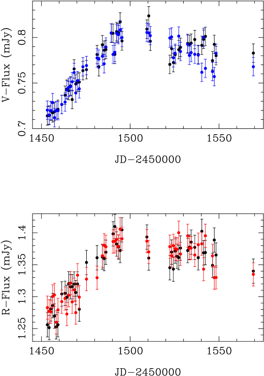
Figure 1: GLITP (black symbols) and SYNa (blue and red symbols) $VR$ light curves. The GLITP fluxes correspond to observations of Q2237+0305A, whereas the SYNa fluxes are synthetic data. In the simulations (SYNa), we take noise processes and sampling consistent with the GLITP photometric errors and dates.

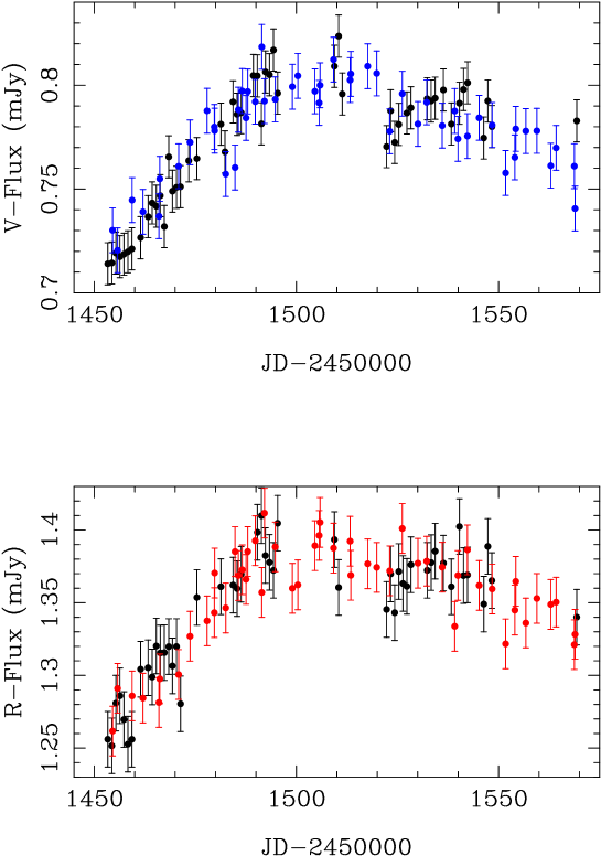
Figure 2: GLITP (black symbols) and SYNd (blue and red symbols) $VR$ light curves. The simulations (SYNd) have a homogeneous sampling.

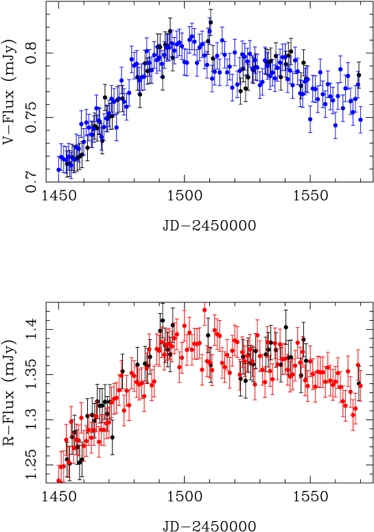
Figure 3: GLITP (black symbols) and SYNe (blue and red symbols) $VR$ light curves. The new synthetic records (SYNe) have a quasi–continuous sampling of one photometric measurement per day.

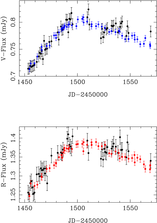
Figure 4: GLITP (black symbols) and SYNf (blue and red symbols) data sets. The simulations (SYNf) have a homogeneous sampling and flux errors two times less than the GLITP ones.

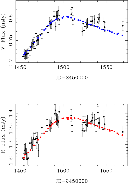
Figure 5: GLITP (black symbols) and SYNg (blue and red symbols) data sets. The simulations (SYNg) have a homogeneous sampling and uncertainties 10 times less than the GLITP errors.

3.2 Synthetic light curves

To study the ability of our scheme, we make synthetic $VR$ light curves and apply the formalism to the simulations (see section 3.3). The GLITP observations of Q2237+0305A are used as a reference data set, which contains 49 fluxes in the $R$ band and 52 fluxes in the $V$ band. The observations were made with the 2.56 m Nordic Optical Telescope (NOT) at Canary Islands (Spain). By pure chance, the component was monitored from day 1450 to day 1575 (in JD–2450000), just during a microlensing peak (Alcalde et al. 2002). In each optical filter, to compute a typical error in the fluxes, the GLITP collaboration used the mean of the absolute differences between adjacent days. Errors of $\sigma_{R}$ = 0.017 mJy and $\sigma_{V}$ = 0.010 mJy were derived from that procedure. We note that our $R$–band calibration is made in an arbitrary way, so our $R$–band fluxes disagree with those in the GLITP Web site. However, the inappropriate calibration is not a problem, because the $q$ estimates do not depend on the calibration of the $VR$ light curves. The amplitudes of the observed features are about 10 times the photometric uncertainties.

Going into details, each underlying signal is generated through the Eq. (13) in Shalyapin et al. (2002). Therefore, a circularly symmetric source model and a caustic crossing are involved. We use a $p$ = 3/2 power–law intensity profile. The source size ratio and the time of caustic crossing by the common center of the sources are taken as $q$ = 0.8 and $t_{0}$ = 1483, respectively. Moreover, the final fluxes are normally distributed around the underlying ones, so the observational random noise is characterized by a normal standard deviation. Except for a family of experiments (those incorporating extremely accurate fluxes), the error bar is computed from the GLITP criterion (the mean of the absolute differences between adjacent fluxes), and it is close to the normal standard deviation. All the simulated $VR$ records have time coverage and flux variations consistent with the GLITP $VR$ records for Q2237+0305A. In the first synthetic experiments, the flux errors and sampling properties agree with the GLITP photometric uncertainties and sampling. The sampling properties are modified in a second kind of experiments, whereas homogeneously distributed and very accurate fluxes are produced in the last experiments.

Firstly, it is considered the SYNa data set. In Figure 1 we have drawn together the observed (GLITP) light curves and the SYNa ones. The black symbols represent the observations, while the blue and red symbols represent the simulations. In SYNa, the standard deviations of the observational noise processes are assumed to be 0.017 mJy ($R$–band) and 0.010 mJy ($V$–band), i.e., in agreement with the GLITP uncertainties. The SYNa sampling also coincides with the GLITP distribution of dates. Indeed, in Fig. 1 we can see synthetic data very similar to the GLITP ones. Besides of this first GLITP–like data set, we generate two more GLITP–like experiments. They are called SYNb and SYNc simulations, and the observations and simulations are again similar in all the details.

An interesting issue is the influence of some observational aspects on the determination of $q$, e.g., the sampling. Therefore, in a second kind of simulations, we exclusively modify the sampling properties. The sampling of the light curves has two main properties: rate and homogeneity. From a ground–based telescope, a sampling rate of one frame each two or three days is excellent. This very good rate is used to generate the first kind of simulations (GLITP–like simulations). The sampling quality also depends on the homogeneity in the dates. For example, the GLITP–like light curves have important gaps. In the SYNd experiment (see Figure 2), we only improve the sampling homogeneity. There are 50 fluxes in each optical band (blue and red symbols in Fig. 2), but their time distributions are highly homogeneous. In another experiment (SYNe) we consider a quasi–continuous sampling of one photometric measurement per day. The GLITP records (black symbols) and the SYNe light curves (blue and red symbols) are showed in Figure 3.

From a third kind of experiments, we can also test the influence of the flux uncertainties. The SYNf $VR$ light curves are generated with normal standard deviations (observational noise processes) of 0.008 mJy ($R$–band) and 0.005 mJy ($V$–band). To produce these synthetic light curves, the sampling rate is assumed to be the GLITP one, the dates are homogeneously distributed along the time coverage, and the flux errors are lowered by a factor of 2. In Figure 4, the black symbols represent the GLITP data, and the blue and red symbols represent the SYNf data. Both data sets (observations and simulations) are similar in some details. However, apart from the sampling homogeneity, it is clear in Fig. 4 that the simulated errors are half the GLITP ones. The SYNg light curves are characterized by normal standard deviations of 1.7 $\mu$Jy ($R$–band) and 1 $\mu$Jy ($V$–band), i.e., with respect to the GLITP–like curves, the uncertainties are lowered by a factor of 10. In Figure 5, we show the two synthetic curves. The accuracy is impressive, and each error bar has a size similar to the point size. In the SYNg experiment, the error bars are not inferred from the usual criterion (the mean of the absolute differences between adjacent fluxes), but they are chosen to be the normal standard deviations. The hypothetical observer cannot measure a flux uncertainty (in a given optical band) from the scatter of fluxes, because the error is clearly smaller than the true day–to–day variability. We assume that the observer uses a non–biased criterion. Moreover, we also use 10 additional experiments similar to SYNf and 10 additional data sets similar to SYNg.

Although our study is mainly based on 27 data sets, we have produced and analyzed about 100 synthetic experiments (”SYN”). The names and properties of the seven basic experiments (see here above) are listed in Table 1.

Name	Sampling rate (data/week)	Homogeneity	$V$–band noise ($\mu$Jy)	$R$–band noise ($\mu$Jy)
SYNa	$\sim$ 3	No	10	17
SYNb	$\sim$ 3	No	10	17
SYNc	$\sim$ 3	No	10	17
SYNd	$\sim$ 3	Yes	10	17
SYNe	7	Yes	10	17
SYNf	$\sim$ 3	Yes	5	8
SYNg	$\sim$ 3	Yes	1	1.7

Table 1: Basic synthetic experiments.

Figure 6: Distributions of $q$ based on NORMAL and BOOTSTRAP repetitions of the SYNa experiment. To derive the BOOTSTRAP repetitions, we use curves smoothed from a 3–point filter (a time window of about 5 days). Dashed lines represent the NORMAL distributions and solid lines trace the BOOTSTRAP histograms. Top panel: minimum $\chi^{2}$ method ($\alpha$ = 2.5 days). Bottom panel: minimum dispersion method ($\delta$ = 2.5 days).

Figure 7: Distributions of $q$ from NORMAL and BOOTSTRAP repetitions of the SYNb experiment (GLITP–like simulations). In the BOOTSTRAP procedure, it is used a 3–point filter (a time window of about 5 days). As remarked in the caption under Fig. 2, dashed lines and solid lines represent the NORMAL and BOOTSTRAP distributions, respectively. Top panel: $\chi^{2}$ ($\alpha$ = 2.5 days). Bottom panel: $D^{2}$ ($\delta$ = 2.5 days).

Figure 8: Histograms based on repetitions of the SYNc experiment (GLITP–like simulations). We present NORMAL (dashed lines) and BOOTSTRAP (solid lines) distributions. We use a 3–point filter in the BOOTSTRAP scheme. Top panel: $\chi^{2}$ ($\alpha$ = 2.5 days). Bottom panel: $D^{2}$ ($\delta$ = 2.5 days).

Figure 9: NORMAL (dashed lines) and BOOTSTRAP (solid lines) histograms associated with repetitions of the GLITP experiment. We show the results from a study with high time resolution: $\alpha$ = $\delta$ = 2.5 days and a 3–point filter.

Figure 10: NORMAL (dashed lines) and BOOTSTRAP (solid lines) histograms associated with repetitions of the SYNd experiment. We show the results from the analysis with $\alpha$ = $\delta$ = 2.5 days and a 3–point filter.

Figure 11: NORMAL (dashed lines) and BOOTSTRAP (solid lines) histograms associated with repetitions of the SYNe experiment. We work with very high time resolution: $\alpha$ = $\delta$ = 1.2 days and a 3–point filter.

Figure 12: NORMAL (dashed lines) and BOOTSTRAP (solid lines) histograms associated with repetitions of the SYNf experiment.

Figure 13: NORMAL (dashed lines) and BOOTSTRAP (solid lines) histograms associated with repetitions of the SYNg experiment.

3.3 Results

Using the experiments in Table 1 together with the scheme in section 3.1 and Appendix A, it might be analyzed the feasibility of an accurate estimate of the source size ratio. We consider a large rectangle in the ($t_{0}$,$q$) plane: 1450 $\leq t_{0}\leq$ 1550 and 0.5 $\leq q\leq$ 1.5, which includes the true values of $t_{0}$ (1483) and $q$ (0.8).

3.3.1 Light curves similar to the GLITP observations

As we have about 50 $VR$ data in a period of 125 days (4 months), the typical separation between adjacent dates is of 2.5 days. Therefore, 2–3 days seems a good range for both the bin semiwidth ($\alpha$) and the decorrelation length ($\delta$). From the SYNa data set, taking $\alpha$ = 2.5 days, the $\chi^{2}$ minimization leads to a best value of $q$ = 1.5 ($t_{0}$ = 1498), whereas from NORMAL and BOOTSTRAP repetitions and the minimum $\chi^{2}$ method, we derive the distributions of $q$ values that appears in Figure 6 (top panel). In order to make the BOOTSTRAP repetitions, we use a 3–point filter. The NORMAL (dashed lines) and BOOTSTRAP (solid lines) distributions are consistent each other. There are dominant peaks at the $q$ = 1.5 edge, secondary features around $q$ = 0.9 and zero probabilities along the $q<$ 0.85 interval. The ratios $q>$ 1 are mainly derived from a relatively small number of $RV$ pairs (in general, $N<$ 40, and sometimes, $N\sim$ 25). Another alternative technique is the minimum dispersion method. When it is applied to the SYNa data (using $\delta$ = 2.5 days), the best value is $q$ = 1.5 ($t_{0}$ = 1523). The new best solution for $q$ is equal to the $\chi^{2}$ best solution for that relevant parameter, and both of them are far from the true value. From NORMAL and BOOTSTRAP repetitions (using a 3–point filter) and $D^{2}$ minimization, new distributions are inferred and showed in Fig. 6 (bottom panel). The new NORMAL (dashed lines) and BOOTSTRAP (solid lines) histograms are very enhanced at the edges. Now, there is not any structure close to $q$ = 0.8. Most the ratios $q\sim$ 0.5 are associated with negative amplifications ($b<$ 0), and some ratios $q\sim$ 1.5 too. The $D^{2}$ results are even worse than the results from the $\chi^{2}$ minimization.

Through the SYNb data, the $\chi^{2}$ best solution is $q$ = 0.98 ($t_{0}$ = 1456), and the results from the $\chi^{2}$ minimization and the repetitions (NORMAL and BOOTSTRAP using a 3–point filter) are presented in Figure 7 (top panel). In all figures, dashed lines trace NORMAL distributions and solid lines describe BOOTSTRAP results. Regarding the distributions in the top panel of Fig. 7, the new histograms are more homogeneous. However, there is zero probability at $q<$ 0.85, and the ratios $q>$ 1 are usually inferred from $N<$ 40 (in some cases, $N\sim$ 25). Sometimes, we simultaneously obtain a value of q larger than one and a negative amplification. On the other hand, the $D^{2}$ best solution is $q$ = 1.5 ($t_{0}$ = 1536). From the minimum dispersion method, we deduce the histograms in Fig. 7 (bottom panel). We remark that there are no repetitions leading to the value $q$ = 0.8 (true ratio), and some extreme values of $q$ ($q\sim$ 0.5 or 1.5) are related to negative amplifications.

Using the SYNc data and $\alpha$ = $\delta$ = 2.5 days, the $\chi^{2}$ and $D^{2}$ best solutions are $q$ = 0.85 ($t_{0}$ = 1535) and $q$ = 0.52 ($t_{0}$ = 1548), respectively. The NORMAL and BOOTSTRAP (3–point filter) histograms are plotted in Figure 8. We note that the results from the SYNc light curves are not very different to the results by means of the SYNa and SYNb data sets. To sum up, with the three experiments (associated with three hypothetical observatories), the distributions from the minimum $\chi^{2}$ technique are not bell–shaped and centered on a ratio near the true value (top panels of Figs. 6–8). Instead of that good behaviour, we obtain rare distributions, which are characterized by the absence of ratios at $q<$ 0.85 and the presence of artifacts in the range 0.85–1.5. The false signals in the 0.85 $\leq q\leq$ 1.5 interval can be distributed in different ways, but curious structures around $q$ = 0.9 are always present. These artifacts are secondary features in the top panel of Fig. 6, prominent features in the top panel of Fig. 7 and dominant structures in Fig. 8 (top panel). In the histograms from the $D^{2}$ minimization (bottom panels of Figs. 6–8), there are dominant peaks at the edges and negligible signals around the true value ($q$ = 0.8). Here as in other parts of the paper, we do not show the results from the $\epsilon^{2}$ minimization (see sections 3.1 and A.3), because the minimum $\epsilon^{2}$ method works better than the $D^{2}$ minimization, but a little worse than the minimum $\chi^{2}$ method. As a global conclusion, using our framework and GLITP–like data sets, we cannot measure the visible–to–red ratio.

Although the simulations consistent with the GLITP observations indicate the non-viability of a measurement of $q$, we compare the best values and distributions from the simulations and the results from the GLITP data. Using the GLITP brightness records, we find that the $\chi^{2}$ ($\alpha$ = 2.5 days) best solution is $q$ = 0.91 ($t_{0}$ = 1546). We also derive the $q$ distributions ($\chi^{2}$) in Figure 9 (top panel). The ratios $q>$ 1 are usually derived through $<$ 40 $RV$ pairs, and in some cases, only $\sim$ 25 $RV$ pairs are used. A slight correlation between large ratios ($q>$ 1) and negative amplifications ($b<$ 0) is another property of the results from the NORMAL and BOOTSTRAP (3–point filter) repetitions. There are no signals at $q<$ 0.85. However, the 0.85–1.5 range includes extended signals and dominant features around $q$ = 0.9. Apart from the $\chi^{2}$ minimization, the $D^{2}$ ($\delta$ = 2.5 days) best solution is $q$ = 0.5 ($t_{0}$ = 1540, $b<$ 0). In Fig. 9 (bottom panel), we show the corresponding $q$ histograms. The ratios $q\sim$ 0.5 are mainly associated with $b<$ 0, and sometimes, $b<0$ for $q>$ 1. Moreover, the distributions are enhanced at the edges. Taking into account the knowledge from the GLITP–like simulations (see here above), all the structures in Fig. 9 could be false features. Even the dominant features in the signals from the minimum $\chi^{2}$ method may be due to the limitations of the framework for the GLITP data set.

3.3.2 Sampling properties

From the SYNd data set (see Table 1) and the techniques, we try to measure the ratio $q$. Using $\alpha$ = 2.5 days, the $\chi^{2}$ best solution is $q$ = 1.24 ($t_{0}$ = 1481). In addition to this best value, the $q$ distributions from the $\chi^{2}$ minimization and 300 repetitions (NORMAL and BOOTSTRAP) are depicted in Figure 10 (top panel). In the BOOTSTRAP procedure, as usual, it is used a 3–point filter. The histograms in the top panel of Fig. 10 are clearly different to the distributions in the top panels of Figs. 6–8. In the new signals, we see dominant structures at $q<$ 0.7 and do not see the artifacts around $q$ = 0.9, which suggests the existence of a relation between the gaps in the GLITP–like curves and the trends in the top panels of Figs. 6–8. In any case, the fraction of ratios in the 0.7–0.9 interval (i.e., the probability that the true value will fall within the 0.7 $\leq q\leq$ 0.9 range) is very small. Therefore, as $P$(0.7 $\leq q\leq$ 0.9) $\leq$ 10% and the true value is $q$ = 0.8, we basically obtain false signals. From the minimum dispersion method, we infer a best ratio of 1.5 ($t_{0}$ = 1525) and deduce the histograms in the bottom panel of Fig. 10. There are dominant peaks at the $q$ = 1.5 edge and very small probabilities at $q<$ 1.2. We remark that the improvement in the sampling homogeneity is not sufficient, since the new best values and $q$ distributions do not permit to estimate the visible–to–red ratio.

By means of either a large collaboration including several observatories around the world or a space telescope, in each optical band, we can get a quasi–continuous sampling of one frame per day. This ”ideal” sampling is assumed in the SYNe experiment. The time resolution is roughly increased by a factor of 2, so 1.2 days is a reasonable choice for both the bin semiwidth ($\alpha$) and the decorrelation length ($\delta$). The $\chi^{2}$ minimization leads to a very promising best value for both the ratio and the time of caustic crossing: $q$ = 0.79 and $t_{0}$ = 1484. However, the distributions of $q$ values have not a behaviour as good as expected. In Figure 11 (top panel), the NORMAL and BOOTSTRAP histograms ($\chi^{2}$) appear. Around $q$ = 0.8, there are prominent peaks with relatively small probabilities of $P$(0.7 $\leq q\leq$ 0.9) $\approx$ 23–24%. These significant features are not dominant structures, but structures surrounded by other similar features. As a result of the existence of several similar features, a fair measurement of $q$ cannot be attained. When the minimum $D^{2}$ method is applied to the SYNe data, the best value is $q$ = 1.48 ($t_{0}$ = 1510). From NORMAL and BOOTSTRAP repetitions and $D^{2}$ minimization, we infer disappointing distributions of $q$ (see the bottom panel of Fig. 11). It becomes apparent the absence of a significant feature in the surroundings of $q$ = 0.8 (true value), and of course, the histograms ($D^{2}$) are strongly biased. Finally, we conclude that our framework does not work in a proper way, even with a substantial improvement in the sampling properties.

3.3.3 Flux errors

In the SYNf experiment, the flux errors are lowered in a factor 2 (see Table 1 and Fig. 4). From the $\chi^{2}$ minimization, taking $\alpha$ = 2.5 days, the best ratio is $q$ = 0.73 ($t_{0}$ = 1489). Using the minimum $\chi^{2}$ technique with the usual time resolution ($\alpha$ = 2.5 days and 3–point filter in BOOTSTRAP repetitions), we obtain two $q$ distributions that are depicted in Figure 12 (top panel). In the top panel of Fig. 12, we see encouraging BOOTSTRAP results. From the BOOTSTRAP repetitions, a dominant peak around $q$ = 0.76 appears. This central value (0.76) is in good agreement with the best ratio (0.73), and moreover, the true ratio (0.8) is included in the $q$ range for the dominant feature. The NORMAL results are worse than the BOOTSTRAP results, because the NORMAL main spike is placed at the $q$ = 0.5 edge. Using the BOOTSTRAP histogram, we can derive the first estimate of the source size ratio. Following the procedure that is described in section 3.1, $q$ = 0.76 $\pm$ 0.05. To obtain the measurement, we ignore the signal at $q<$ 0.6 and $q>$ 0.9. However, unfortunately, the possibility of $\sim$ 3–10% measurements of the source size ratio is not supported by other experiments similar to the SYNf one. For example, from ten new synthetic experiments and the $\chi^{2}$ minimization, only three best ratios are included in the promising 0.65 $\leq q\leq$ 0.85 interval. In five cases, the best ratio is of about 0.5, whereas in two cases, the best value is close to 1.4. Therefore, if we consider ten hypothetical observers measuring the source size ratio each of them (via $\chi^{2}$/BOOTSTRAP), several best estimates and distributions of $q$ will be in serious disagreement with the true ratio. Although some particular observers are successful, most observers fail in the determination of $q$. Through the SYNf–like experiments, we also derive $\chi^{2}_{min}$ values in the interval 0.25–0.60. These results suggest that we deal with seven biased ”superfits”, which are not related to the true physical scenario. The observational noise and discontinuous sampling are the cause of the superb correlations between the $V$ fluxes and the $R$ ones. From the minimum dispersion method, taking $\delta$ = 2.5 days, the best ratio is $q$ = 1.15 ($t_{0}$ = 1523). The NORMAL and BOOTSTRAP repetitions lead to poor histograms. These $D^{2}$ histograms appear in Fig. 12 (bottom panel). In spite of the small peak in the surroundings of the true value, it is apparent that the distributions are biased. From the NORMAL and BOOTSTRAP distributions of $q$ ($D^{2}$), a false ratio exceeding the critical value ($q$ = 1) is strongly favoured. If we compare the results in Fig. 12 and the distributions in Fig. 10 (from a data set with similar sampling and larger errors), it is clear that the decrease of the flux errors leads to a global improvement. With smaller errors, we find stronger signals in the proximity of the true ratio.

As the photometric errors seem to have a significant influence on the $q$ distributions, finally, we explore the ability of the methodology with extremely accurate photometric data. For this final effort, the SYNg data set is a suitable tool. For the SYNg data, the $\chi^{2}$ minimization gives a best solution: $q$ = 0.79 ($t_{0}$ = 1484), while for the NORMAL and BOOTSTRAP repetitions, the technique also works well. In Figure 13 (top panel), the corresponding distributions are plotted. We see dominant structures around $q$ = 0.80 (NORMAL and BOOTSTRAP central value). With the $q$ resolution in the top panel of Fig. 13, the main features have not a nice shape, but they contain most the best solutions. Our $\chi^{2}$/NORMAL&BOOTSTRAP measurement is of $q$ = 0.80 $\pm$ 0.08 (ignoring the signal at $q<$ 0.65 and $q>$ 0.95). From ten monitorings similar to the SYNg experiment and the minimum $\chi^{2}$ method, we get convincing results: nine best ratios are within the 0.70 $\leq q\leq$ 0.92 interval, and only one best ratio has a biased value of $q$ = 0.52. Even in this last case ($q$ = 0.52), the NORMAL and BOOTSTRAP histograms have relatively good behaviours. The NORMAL distribution shows a dominant spike close to 0.5, which contains about 50% of the best ratios. However, the rest of ratios (about 50%) are mainly placed in the 0.65 $\leq q\leq$ 0.95 range. In the BOOTSTRAP distribution, there is also an extended feature within the 0.65 $\leq q\leq$ 0.95 range, which includes about 70% of the ratios. The highest spike at $q\sim$ 0.5 only contains about 30% of the ratios. In other words, the hypothetical observer would find doubtful results, since there are evidences for two different values: $q\sim$ 0.5 (artifact) and $q\sim$ 0.8 (true ratio). Apart from this troublesome situation, any possible observer has a very high probability (about ninety per cent) of measuring a fair and accurate visible–to–red ratio ($\sim$ 10% measurement). For the nine SYNg–like experiments leading to non–biased values of $q$, the $\chi^{2}_{min}$ varies from 0.95–1.20, i.e., we infer a reasonable $\chi^{2}_{min}$ interval and all is ok. However, $\chi^{2}_{min}$ = 0.6 from the SYNg–like experiment associated with a strange value of $q$. The strange ratio is related to a very small $\chi^{2}$ (”superfit”), and both ($\chi^{2}_{min}$ and $q$) are due to the noise and sampling. From the minimum $D^{2}$, the best ratio is $q$ = 0.80 ($t_{0}$ = 1484). This is the only case in which both the $\chi^{2}$ and $D^{2}$ best estimates are nearby each other and the true value. New $D^{2}$ histograms appear in Fig. 13 (bottom panel). The two distributions in the bottom panel of Fig. 13 are really rare. We see the true signal inside the 0.65 $\leq q\leq$ 0.95 interval and other features at $q>$ 1. The main structures are related to ratios in the $\sim$ 1.1–1.4 range. Why are the $D^{2}$ histograms so rare?. From the 10 synthetic data sets similar to the SYNg one and the minimum $D^{2}$ method, we infer surprising results: two ratios exceeding the critical value (i.e., larger than 1) and eight ratios larger than 0.74 and smaller than 0.91. This independent $q$ distribution (based on real repetitions, i.e., using the true underlaying signal) indicates that the NORMAL and BOOTSTRAP procedures may be unsuitable with extremely accurate light curves and the $D^{2}$ minimization. Finally, we note that future monitoring projects from modern ground–based or space telescopes can lead to $\sim$ 10% measurements of the visible–to–red ratio. To be successful in the accurate determination of $q$, a reasonable sampling and a few $\mu$Jy uncertainties are required.

4 Summary and discussion

We present a new framework to analyze the structure of the optical compact source of a lensed QSO. When a microlensing high–magnification event (HME) is produced in one of the QSO components, assuming that the compact emission regions have different sizes in different wavelengths, the multiband light curves of the HME can be used to measure the source size ratios (e.g., Wambsganss & Paczyński 1991). In this paper, we deal with a kind of HMEs: the special high–magnification events (SHMEs). This family includes the well–known caustic crossing as well as other situations, e.g., the two–dimensional maximum crossing. Our method has the advantage that finds the source size ratios in a direct and model–independent (stationary source model) way and without complex computation procedures. From the brightness records of a caustic crossing event (CCE), the deconvolution technique leads to a richer information, because the method enables to retrieve the one–dimensional intrinsic luminosity profiles (e.g., Grieger, Kayser & Schramm 1991). However, the determination of the 1D intrinsic luminosity profiles is not a fair and simple task, and the problem is related to complex inversion procedures. To infer a source size ratio, we propose a straightforward cross–correlation between the records in the two optical bands, so our procedure has some resemblance to the classical time delay measurement. In order to measure the visible–to–red ratio ($q=R_{V}/R_{R}$), we also introduce several suitable tools, which can be applied to derive another ratio ($R_{U}/R_{B}$, $R_{B}/R_{V}$, …).

The power of the new scheme is tested from synthetic light curves that are related to the $V$–band and $R$–band GLITP microlensing peaks in the flux of Q2237+0305A (Alcalde et al. 2002). Very recently, assuming that the GLITP/Q2237+0305A fluctuations are due to a CCE, Shalyapin et al. (2002) and Goicoechea et al. (2003) analyzed the nature and size of the optical compact source, as well as the central mass and accretion rate associated with the favoured model (standard accretion disk). In this work, the GLITP/Q2237+0305A records are also associated with a CCE (for a discussion on the origin of the GLITP/Q2237+0305A data set, see here below). To generate synthetic datasets, we take underlying signals in agreement with the GLITP observations (reduced $\chi^{2}$ values close to 1). They correspond to $p$ = 3/2 power–law source profiles crossing a fold caustic, so the source size ratio is taken as $q$ = 0.8 (see Tables 1–3 in Shalyapin et al. 2002). Once an underlying signal is made, we add observational random noise, which is characterized by a normal standard deviation. This random noise must incorporate the pure observational uncertainty and the day–to–day intrinsic variability. We remark that the scheme is based on a stationary source model, and thus, the underlying signal cannot include any intrinsic variation. While in some synthetic experiments, the flux errors and sampling properties agree with the GLITP photometric uncertainties and sampling, in other experiments, the influence of the sampling properties and flux errors is studied in detail. We find that GLITP–like datasets are not suitable for measuring the visible–to–red ratio. Even with a dramatic improvement in the sampling, our framework does not lead to convincing results. However, if the flux uncertainties are significantly lowered, the scheme works in an accurate way. From $VR$ light curves with a few $\mu$Jy uncertainties, we can infer $\sim$ 10% measurements of $q$. Assuming the NOT uncertainties for Q2237+0305A (of about 10 $\mu$Jy) as mainly due to pure observational noise, it would be viable to achieve smaller errors using the current superb–telescopes (the best ground–based telescopes or the Hubble Space Telescope). Therefore, there are no technological obstacles to get accurate estimates of the visible–to–red ratio for QSO 2237+0305. The possible presence of very rapid intrinsic variability with relatively large amplitude would be the only serious obstacle. Using the $\chi^{2}$ minimization, one can obtain an accurate value of $q$ in two ways: either from only one monitoring and standard techniques to infer the error in $q$, or from the best solutions corresponding to several datasets of different observatories. However, using the minimum dispersion method, the standard repetitions of an individual experiment do not seem to lead to good results, and one must focus on the best solutions from different experiments. In general, the $\chi^{2}$ minimization works better than the minimum dispersion method, and the $\epsilon^{2}$ minimization is a technique with intermediate quality.

Sampling and flux errors aside, other factors may determine the ability of the methodology. For example, the time coverage of the SHME. We only test microlensing peaks lasting $\sim$ 100 days, but longer and larger variations could lead to an accurate determination of the ratio, without need for improving the uncertainties. Nevertheless, it is hard to imagine a long period of about 1 year in which the source QSO does not vary. From a long–timescale monitoring, we would observe a dirty SHME, i.e., true microlensing fluctuations that are contaminated by some intrinsic variation. Moreover, it may be difficult to detect a pure SHME, since a long–timescale event may include variability from either several features in the magnification pattern or random stellar motions in the deflector. Another possibility is the determination of $q$ from very fast microlensing events. For a given level of noise, some probes indicate that the fastest underlaying signals enable the best measurements of the ratio. Therefore, faster events in Q2237+0305A as well as very fast events in another component of that system or other lensed QSO would represent more favourable situations.

Before to reliably apply the scheme, a key point is to confirm that the observed records are very probably related to a clean and pure SHME. This task is not so easy, and currently, even the origin of the GLITP/Q2237+0305A fluctuations is not a totally clear matter. The global flat shape for the $VR$ GLITP light curves of Q2237+0305D (the faintest component of the system) indicates the absence of a global intrinsic variation. Therefore, the GLITP/Q2237+0305A peaks seem to be clean microlensing fluctuations. On the other hand, the $V$–band and $R$–band GLITP light curves of Q2237+0305A trace the regions around the maxima of the $VR$ fluctuations. As the peaks are highly asymmetric and correspond to a prominent event (observations by the OGLE team), they were associated with a CCE (a kind of SHME) since were discovered. The CCE hypothesis led to very reasonable results for the source structure (Shalyapin et al. 2002; Goicoechea et al. 2003) , which are an a posteriori support for the initial hypothesis. But do they really correspond to a pure CCE?. Kochanek (2004) studied the source trajectories that agree with the whole $V$–band OGLE light curves for Q2237+0305A–D. His results for the origin of the prominent event in the A component are a bit disappointing, because the best trajectories in terms of $\chi^{2}$ cross over simple folds, but other relatively good trajectories pass through complex magnification zones (see Figs. 12–16 in Kochanek 2004). However, several issues suggest that the Kochanek’s conclusions about the nature of the microlensing event are preliminary ones. First, the conclusions were based on a joint study of the four components A–D during a long period. Second, it was used an enlargement of the formal errors, so the pair of best trajectories on the magnification patterns for Q2237+0305A have excessively small values of $\chi^{2}$ ($\chi^{2}_{0}=186-187$, $N_{dof}$ = 290), and the rest of good paths are characterized by $\Delta\chi^{2}=\chi^{2}-\chi^{2}_{0}\geq 14-15$. In the circumstances, the use of smaller uncertainties does not seem unrealistic. Moreover, the new uncertainties could lead to $\Delta\chi^{2}>(2N_{dof})^{1/2}$. Third, in order to obtain statistical conclusions, the total number of good trajectories is clearly small. At present, the University of Cantabria group is carrying out a deep study about the origin of the OGLE–GLITP/Q2237+0305A event.

Appendix A Minimization techniques

A.1 $\chi^{2}$ minimization

The whole data set includes the observed fluxes in the $R$ band, $F_{R}(t_{i})$, $i=1,2,...,N_{R}$, with common uncertainties $\sigma_{R}$, and the observed fluxes in the $V$ band, $F_{V}(t_{j})$, $j=1,2,...,N_{V}$, with observational errors $\sigma_{V}$. The $R$–band flux at time $t_{i}$, $F_{R}(t_{i})$, is compared to the flux $a+bF_{V}(t^{\prime}_{i})$, where $t^{\prime}_{i}=qt_{i}+(1-q)t_{0}$. In general, the dilated and delayed time $t^{\prime}_{i}$ does not coincide with any epoch in the $V$ band, and we estimate the value of $F_{V}(t^{\prime}_{i})$ by averaging the $V$–band fluxes within the bin centered on $t^{\prime}_{i}$ with a semiwidth $\alpha$. To average, it is appropriate the use of weights depending on the separation between the central time $t^{\prime}_{i}$ and the dates $t_{j}$ in the bin. For given values of $q$ and $t_{0}$, the number of possible [$F_{R}(t_{i})$,$F_{V}(t^{\prime}_{i})$] pairs is less or equal to $N_{R}$, since some $V$–band bins may be empty. The $\chi^{2}$ estimator is given by

$$\chi^{2}(a,b,t_{0},q)=\frac{1}{N-4}\sum_{i=1}^{N}\frac{[F_{R}(t_{i})-a-bF_{V}(t^{\prime}_{i})]^{2}}{\sigma_{R}^{2}+b^{2}\sigma_{Vi}^{2}},$$ (9)

where $N$ is the number of $RV$ pairs ($N\leq N_{R}$), $F_{V}(t^{\prime}_{i})=[\sum_{j}S_{ij}F_{V}(t_{j})]/\sum_{j}S_{ij}$, the weight–selection factors $S_{ij}$ are

$$S_{ij}=\left\{\begin{aligned} 1-\frac{|t^{\prime}_{i}-t_{j}|}{\alpha},\;\;\rm if\it\;|t^{\prime}_{i}-t_{j}|\leq\alpha,\\ 0,\;\,\rm if\it\;|t^{\prime}_{i}-t_{j}|>\alpha,\end{aligned}\right.$$ (10)

and the uncertainties in the fluxes $F_{V}(t^{\prime}_{i})$ are

$$\sigma_{Vi}^{2}=\frac{\sum_{j}S_{ij}^{2}\sigma_{V}^{2}}{(\sum_{j}S_{ij})^{2}}.$$ (11)

In principle, the $\chi^{2}$ estimator is a function of four parameters $(a,b,t_{0},q)$. However, as the parameter $a$ is entered in Eq. (A.1) in a simple way, it is possible to obtain an analytical constraint $a=a(b,t_{0},q)$ from the minimization condition $\partial\chi^{2}/\partial a=0$. One finds $a=P-bQ$, where

$$P=\left[\sum_{i=1}^{N}\frac{F_{Ri}}{\sigma_{R}^{2}+b^{2}\sigma_{Vi}^{2}}\right]/\left[\sum_{i=1}^{N}\frac{1}{\sigma_{R}^{2}+b^{2}\sigma_{Vi}^{2}}\right],$$ (12)

and

$$Q=\left[\sum_{i=1}^{N}\frac{F_{Vi}}{\sigma_{R}^{2}+b^{2}\sigma_{Vi}^{2}}\right]/\left[\sum_{i=1}^{N}\frac{1}{\sigma_{R}^{2}+b^{2}\sigma_{Vi}^{2}}\right].$$ (13)

Thus, we search for the minimum of $\chi^{2}$ in a 3D parameter space, i.e., we minimize the function $\chi^{2}=\chi^{2}[a(b,t_{0},q),b,t_{0},q]$.

A.2 Minimum dispersion method

Our $R$–band data are modelled as $F_{Ri}=s(t_{i})+\epsilon_{R}(t_{i})$. Here, $s$ and $\epsilon_{R}$ denote the true $R$–band signal and the unknown $R$–band errors, respectively. In a consistent way (see Eqs. 6 and 8), the $V$–band data should be modelled as $F_{Vj}=\{s[t_{j}/q+(1-1/q)t_{0}]-a\}/b+\epsilon_{V}(t_{j})$. These two series are combined into one for every fixed value of an offset $a$, an amplification $b$, a characteristic time $t_{0}$ and a dilation factor $q$. In the combined serie, $N_{R}$ data are the $F_{Ri}$ values at times $t_{i}$, whereas the rest of data ($N_{V}$) are the $a+bF_{Vj}$ values at dates $t^{\prime}_{j}=t_{j}/q+(1-1/q)t_{0}$. Each combined curve includes $N_{R}+N_{V}$ fluxes and times. The dispersion of the combined curve is

$$D^{2}(a,b,t_{0},q)=\frac{\sum_{i=1}^{N_{R}}\sum_{j=1}^{N_{V}}S_{ij}W_{ij}(F_{Ri}-a-bF_{Vj})^{2}}{\sum_{i=1}^{N_{R}}\sum_{j=1}^{N_{V}}S_{ij}W_{ij}},$$ (14)

where $S_{ij}$ are weight–selection factors defined by

$$S_{ij}=\left\{\begin{aligned} 1-\frac{|t_{i}-t^{\prime}_{j}|}{\delta},\;\;\rm if\it\;|t_{i}-t^{\prime}_{j}|\leq\delta,\\ 0,\;\,\rm if\it\;|t_{i}-t^{\prime}_{j}|>\delta,\end{aligned}\right.$$ (15)

and $W_{ij}=1/(\sigma_{R}^{2}+b^{2}\sigma_{V}^{2})$ are the statistical weights. We note that all the ($i$,$j$) pairs have equal statistical weight, and in this special case, the $W_{ij}$ factors do not play a role in the $D^{2}$ estimator. The main difference between the old problem (estimation of the best time delay) and the new one (estimation of the best source size ratio) lies in the dilation factor that is absent in delay studies.

In the minimization process, one can also reduce the dimension of the parameter space (see the end of section A.1). We search for the minimum dispersion in a 2D parameter space, since there are analytical constraints $a=a(t_{0},q)$ and $b=b(t_{0},q)$. These constraints are inferred from the system of equations: $\partial D^{2}/\partial a=\partial D^{2}/\partial b=0$. In a straightforward way, the system leads to $a=P-bQ$ and $b=(X-PQ)/(S-Q^{2})$, being

$$P=\sum_{i}\sum_{j}S_{ij}F_{Ri}/\sum_{i}\sum_{j}S_{ij},$$ (16)

$$Q=\sum_{i}\sum_{j}S_{ij}F_{Vj}/\sum_{i}\sum_{j}S_{ij},$$ (17)

$$S=\sum_{i}\sum_{j}S_{ij}F_{Vj}^{2}/\sum_{i}\sum_{j}S_{ij},$$ (18)

$$X=\sum_{i}\sum_{j}S_{ij}F_{Ri}F_{Vj}/\sum_{i}\sum_{j}S_{ij}.$$ (19)

A.3 Minimum modified dispersion method

We also propose a modified dispersion. The basic difference lies in the fact that we do not use the usual terms $(F_{Ri}-a-bF_{Vj})^{2}$, but the normalized ones $(F_{Ri}-a-bF_{Vj})^{2}/(\sigma_{R}^{2}+b^{2}\sigma_{V}^{2})$. The new estimator has an expression

$$\epsilon^{2}(a,b,t_{0},q)=\frac{\sum_{i=1}^{N_{R}}\sum_{j=1}^{N_{V}}S_{ij}W_{ij}(F_{Ri}-a-bF_{Vj})^{2}}{\sum_{i=1}^{N_{R}}\sum_{j=1}^{N_{V}}S_{ij}}.$$ (20)

The $\epsilon^{2}$ estimator depends on four parameters: $a$, $b$, $t_{0}$ and $q$, but we can use some constraints and simplify the 4D minimization process. From $\partial\epsilon^{2}/\partial a=0$, it is inferred the relationship

$$a=\frac{\sum_{i}\sum_{j}S_{ij}(F_{Ri}-bF_{Vj})}{\sum_{i}\sum_{j}S_{ij}}.$$ (21)

If we denote the averages of the light curves as

$$P=\sum_{i}\sum_{j}S_{ij}F_{Ri}/\sum_{i}\sum_{j}S_{ij},\ \ Q=\sum_{i}\sum_{j}S_{ij}F_{Vj}/\sum_{i}\sum_{j}S_{ij},$$ (22)

then the expression for the parameter $a$ takes the simple appearance

$$a=P-bQ.$$ (23)

Using $\partial\epsilon^{2}/\partial b=0$, it is derived a second interesting constraint. The new constraint can be written as

$$\sum_{i}\sum_{j}S_{ij}(F_{Ri}-a-bF_{Vj})\left(b\sigma_{V}^{2}F_{Ri}+\sigma_{R}^{2}F_{Vj}\right)=0.$$ (24)

In order to simplify the expression (A.16), we introduce the deviations of the fluxes from the averages. Thus,

$$\delta F_{Ri}=F_{Ri}-P,\ \ \delta F_{Vj}=F_{Vj}-Q.$$ (25)

From Eqs. (A.15), (A.16) and (A.17), we finally obtain

$$\begin{split}-b^{2}\sigma_{V}^{2}\sum_{i}\sum_{j}S_{ij}F_{Ri}\delta F_{Vj}+b\left(\sigma_{V}^{2}\sum_{i}\sum_{j}S_{ij}F_{Ri}\delta F_{Ri}-\sigma_{R}^{2}\sum_{i}\sum_{j}S_{ij}F_{Vj}\delta F_{Vj}\right)+\\ \sigma_{R}^{2}\sum_{i}\sum_{j}S_{ij}F_{Vj}\delta F_{Ri}=0.\end{split}$$ (26)

Now it is clear that one can work in a 2D parameter space. For a given pair ($t_{0}$,$q$), through Eqs. (A.15) and (A.18), we can straightway derive the solutions ($a$,$b$) that minimize the $\epsilon^{2}$ estimator.