The Size Distribution of Kuiper Belt Objects

Abstract

We describe analytical and numerical collisional evolution calculations for the size distribution of icy bodies in the Kuiper Belt. For a wide range of bulk properties, initial masses, and orbital parameters, our results yield power-law cumulative size distributions, $N_{C}\propto r^{-q}$, with $q_{L}\approx$ 3.5 for large bodies with radii, $r\gtrsim$ 10–100 km, and $q_{s}\approx$ 2.5–3 for small bodies with radii, $r\lesssim$ 0.1–1 km. The transition between the two power laws occurs at a break radius, $r_{b}\approx$ 1–30 km. The break radius is more sensitive to the initial mass in the Kuiper Belt and the amount of stirring by Neptune than the bulk properties of individual Kuiper Belt objects (KBOs). Comparisons with observations indicate that most models can explain the observed sky surface density $\sigma(m)$ of KBOs for red magnitudes $R\approx$ 22–27. For $R\lesssim$ 22 and $R\gtrsim$ 28, the model $\sigma(m)$ is sensitive to the amount of stirring by Neptune, suggesting that the size distribution of icy planets in the outer solar system provides independent constraints on the formation of Neptune.

1 INTRODUCTION

The Kuiper Belt is a vast swarm of icy bodies beyond the orbit of Neptune in our solar system. Following the discovery of the first Kuiper Belt objects (KBOs) in 1930 (Pluto; Tombaugh, 1946) and 1992 (1992 QB₁; Jewitt & Luu, 1993), several groups began large-scale surveys to characterize the limits of the Kuiper Belt (e.g., Luu et al, 1997; Allen et al., 2001; Gladman et al., 2001; Larsen et al., 2001, and references therein). Today, there are 800–1000 known KBOs with radii $r\gtrsim$ 50 km in orbits that extend from 35 AU out to at least 150 AU (Luu & Jewitt, 2002; Bernstein et al., 2003). The vertical scale height of the KBO population is $\sim$ 20–30 deg. The total mass is $\sim$ 0.01–0.1 $M_{\oplus}$ (Luu & Jewitt, 2002).

Observations place numerous constraints on the apparent size distribution of KBOs. Deep imaging surveys at $R\approx$ 22–28 suggest a power-law cumulative size distribution, $N_{C}\propto r^{-q_{o}}$, with $q_{o}=3.0\pm 0.5$ (Trujillo, Jewitt, & Luu, 2001; Luu & Jewitt, 2002). Data from the ACS on HST suggest a change in the slope of the size distribution at a break radius $r_{b}\sim$ 10–30 km (Bernstein et al., 2003). Dynamical considerations derived from the orbits of Pluto-Charon and Jupiter family comets suggest $r_{b}\sim$ 1–10 km (Duncan et al., 1988; Levison & Duncan, 1994; Levison & Stern, 1995; Duncan et al., 1995; Duncan & Levison, 1997; Ip & Fernández, 1997; Stern, Bottke & Levison, 2003). Observations of the optical and far-infrared background light require $q_{o}\lesssim$ 2.5 for small objects with radii $\lesssim$ 0.1–1 km (Backman, Dasgupta, & Stencel, 1995; Stern, 1996b; Teplitz et al., 1999; Kenyon & Windhorst, 2001), suggesting $r_{b}\gtrsim$ 0.1–1 km.

These observations provide interesting tests of planet formation theories. In the planetesimal hypothesis, planetesimals with radii $\lesssim$ 1–10 km collide, merge, and grow into larger objects. This accretion process yields a power-law size distribution, $N_{C}\propto r^{-q}$, with $q_{L}\approx$ 2.8–3.5 for 10–100 km and larger objects (Kenyon & Luu, 1999b; Kenyon, 2002). As the largest objects grow, their gravity stirs up the orbits of leftover planetesimals to the disruption velocity. Collisions between leftover planetesimals then produce fragments instead of mergers. For objects with radii of 1–10 km and smaller, this process yields a power-law size distribution with a shallower slope, $q_{S}\approx$ 2.5 (Stern, 1996a; Davis & Farinella, 1997; Stern & Colwell, 1997a, b; Kenyon & Luu, 1999a; Kenyon & Bromley, 2004).

Despite uncertainties in the observations and the theoretical calculations, the predicted power-law slopes for large and small KBOs agree remarkably well with the data. However, many issues remain. The observed sky surface density of the largest objects with radii of 300–1000 km and the location of the break in the size distribution are uncertain (see, for example, Luu & Jewitt, 2002; Bernstein et al., 2003). The data also suggest that different dynamical classes of KBOs have different size distributions (Levison & Stern, 2001; Bernstein et al., 2003). Theoretical models for the formation of KBOs have not addressed this issue. Theoretical predictions for $r_{b}$, $q_{S}$, and the space density of KBOs are also uncertain. Observations indicate that the observed space density of KBOs is $f\lesssim$ 1% of the initial density of solid material in the planetesimal disk. Theoretical estimates of long-term collisional evolution yield $f\lesssim$ 10% (e.g., Stern & Colwell, 1997b; Kenyon, 2002), but the sensitivity of this estimate to the bulk properties of KBOs has not been explored in detail.

Here, we consider collision models for the formation and long-term collisional evolution of KBOs in the outer solar system. We use an analytic model to show how the break radius depends on the bulk properties and orbital parameters of KBOs (see Pan & Sari, 2004, for a similar analytic model) and confirm these estimates with numerical calculations. If KBOs have relatively small tensile strengths and formed in a relatively massive solar nebula, we derive a break radius, $r_{b}\sim$ 3–30 km, close to the observational limits. The numerical calculations also provide direct comparisons with the observed sky surface density and the total mass in the Kuiper Belt. Models with relatively weak KBOs and additional stirring by Neptune yield the best agreement with observations and make testable predictions for the surface density of KBOs at $R\approx$ 28–32. In the next 3–5 yr, occultation observations can plausibly test these predictions.

We develop the analytic model in §2, describe numerical simulations of KBO evolution in §3, and conclude with a brief discussion and summary in §4.

2 ANALYTIC MODEL

2.1 Derivation

We begin with an analytic collision model for the long-term evolution of an ensemble of KBOs. We assume that KBOs lie in an annulus of width $\Delta a$ centered at a heliocentric distance $a$. KBOs with radius $r$ orbit the Sun with eccentricity $e$ and inclination $i$. The scale height $H$ of the KBO population is $H$ = $a$ sin $i$.

KBOs evolve through collisions and long range gravitational interactions. Here, we assume that gravitational interactions have reached a steady-state, with $e$ and $i$ constant in time. Based on numerical simulations of KBO formation, we adopt a broken power law for the initial size distribution,

$$n(r)=\left\{\begin{array}[]{l l l}n_{S}r^{-\alpha_{S}}&&r\leq 1~{}{\rm km}\\ \\ n_{L}r^{-\alpha_{L}}&&r\geq 1~{}{\rm km}\\ \end{array}\right.$$ (1)

with $\alpha_{S}$ = 3.5 for small objects and $\alpha_{L}$ = 4.0 for large objects (Stern & Colwell, 1997a; Davis & Farinella, 1997; Stern & Colwell, 1997b; Kenyon & Luu, 1999a; Kenyon, 2002; Kenyon & Bromley, 2004). If $V$ is the relative velocity, the collision rate for a KBO with radius $r_{1}$ and all KBOs with radius $r_{2}$ is

$$\frac{dn_{1}}{dt}=\left(\frac{n_{2}}{4~{}H~{}a~{}\Delta a}\right)~{}\left(1+2.7\frac{V_{e}^{2}}{V^{2}}\right)~{}V~{}(r_{1}+r_{2})^{2}~{},$$ (2)

where $V_{e}$ is the escape velocity of a single body with mass, $m=m_{1}+m_{2}$ (Wetherill & Stewart, 1993; Kenyon & Luu, 1998, and references therein).

The collision outcome depends on the impact velocity $V_{I}$ and the disruption energy $Q_{d}$. We follow previous investigators and define the energy needed to remove 50% of the combined mass of two colliding planetesimals,

$$Q_{d}=Q_{b}r^{\beta_{b}}+\rho Q_{g}r^{\beta_{g}}~{},$$ (3)

where $Q_{b}r^{\beta_{b}}$ is the bulk (tensile) component of the binding energy and $\rho Q_{g}r^{\beta_{g}}$ is the gravity component of the binding energy (see, for example, Davis et al., 1985; Wetherill & Stewart, 1993; Holsapple, 1994; Benz & Asphaug, 1999; Housen & Holsapple, 1999). The gravity component of the disruption energy varies linearly with the mass density $\rho$ of the planetesimals. This expression ignores a weak relation between $Q_{b}$,$Q_{g}$ and the impact velocity $V_{I}$

$$Q_{b},Q_{g}\propto\left(\frac{V_{I}}{V_{0}}\right)^{\beta_{v}}~{},$$ (4)

where $\beta_{v}\approx$ 0.25–0.50 for rocky material and $\beta_{v}\approx$ $-0.25$ to $-0.50$ for icy material (e.g. Housen & Holsapple, 1990, 1999; Benz & Asphaug, 1999). For an analytic model with $V_{I}$ = constant, the variation of $Q_{d}$ with $V_{I}$ is not important. We consider non-zero $\beta_{v}$ in complete evolutionary calculations described below.

We adopt the standard center of mass collision energy (Wetherill & Stewart, 1993)

$$Q_{I}=\frac{m_{1}m_{2}V_{I}^{2}}{4(m_{1}+m_{2})^{2}}~{},$$ (5)

where the impact velocity is

$$V_{I}^{2}=V^{2}+V_{e}^{2}~{}.$$ (6)

The mass ejected in a collision is

$$m_{ej}=0.5(m_{1}+m_{2})\left(\frac{Q_{I}}{Q_{d}}\right)^{\beta_{e}}~{},$$ (7)

where $\beta_{e}$ is a constant of order unity (see Davis et al., 1985; Wetherill & Stewart, 1993; Kenyon & Luu, 1998; Benz & Asphaug, 1999, and references therein).

For a single KBO, the amount of mass accreted in collisions with all other KBOs during a time interval $\delta t$ is

$$\delta m_{a}(r)=\dot{m_{a}}~{}\delta t=\delta t~{}\int\frac{dn_{1}}{dt}~{}m_{2}~{}dm_{2}~{}.$$ (8)

The amount of mass lost is

$$\delta m_{l}(r)=\dot{m_{l}}~{}\delta t=\delta t~{}\int\frac{dn_{1}}{dt}~{}m_{ej}~{}dm_{2}~{}.$$ (9)

KBOs with $\dot{m_{l}}>\dot{m_{a}}$ lose mass and reach zero mass on a removal timescale

$$t_{r}(r)\approx\frac{m_{0}(r)}{\dot{m_{l}}-\dot{m_{a}}}~{}.$$ (10)

With these definitions, the evolution of an ensemble of KBOs depends on the relative velocity $V$, the size distribution, and the disruption energy. Because the disruption energy scales with size, larger objects are harder to disrupt than smaller objects. To produce a break in the size distribution, we need a ‘break radius,’ $r_{b}$, where

$$\begin{array}[]{l l l}t_{r}\leq t_{0}&&{\rm for}~{}r\leq r_{b}\\ \\ t_{r}>t_{0}&&{\rm for}~{}r>r_{b}\\ \end{array}.$$ (11)

and $t_{0}$ is some reference time. We choose $t_{0}$ = 1 Gyr as a reasonable e-folding time for the decline in the KBO space density.

2.2 Application

To apply the analytic model to the KBO size distribution, we use parameters appropriate for the outer solar system. We adopt $i$ = $e$/2, with $e$ = 0.04 for classical KBOs and $e$ = 0.2 for Plutinos. This simplification ignores the richness of KBO orbits, but gives representative results without extra parameters. We assume a total mass in KBOs, $M_{KBO}$, in an annulus with $a_{0}$ = 40 AU and $\delta a$ = 10 AU. A minimum mass solar nebula has $M_{KBO}\sim$ 10 $M_{\oplus}$; the current Kuiper Belt has $M_{KBO}$ = 0.05–0.20 $M_{\oplus}$ (Stern, 1996a; Luu & Jewitt, 2002; Bernstein et al., 2003). This range in initial KBO mass provides a representative range for the normalization constants, $n_{S}$ and $n_{L}$, in our model size distribution.

To model the destruction of KBOs, we adopt representative values for $Q_{b}$, $Q_{g}$, $\beta_{b}$, $\beta_{g}$, and $\rho$. Because the bulk properties of KBOs are poorly known, we consider wide ranges in $Q_{b}=10^{1}$ to $10^{8}$ erg g ^-1, $C_{g}=\rho Q_{g}$ = $10^{-4}$ to $10^{4}$ erg g^-1, and $\beta_{g}$ = 0.5–2.0. These ranges span analytic and numerical results in the literature (e.g., Davis et al., 1985; Holsapple, 1994; Love & Ahrens, 1996; Benz & Asphaug, 1999; Housen & Holsapple, 1999). For simplicity, we adopt $\beta_{b}$ = 0; other choices have little impact on the results.

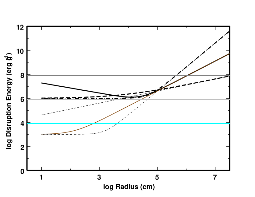
Figure 1: Comparison of catastrophic disruption energy for models described by equation (3) with $\rho$ = 1.5 g cm^-3. Solid curve: $Q_{b}=1.6\times 10^{7}$ erg g^-1, $Q_{g}=1.5$ erg g^-1, $\beta_{b}$ = $-0.42$, $\beta_{g}$ = 1.25 (Benz & Asphaug, 1999). Dot-dashed curves: $Q_{g}=2.67\times 10^{-4}$ erg g^-1, $\beta_{b}$ = $0$, $\beta_{g}$ = 2 (Davis et al., 1985). Dashed curves: $Q_{g}=8.4\times 10^{3}$ erg g^-1, $\beta_{b}$ = $0$, $\beta_{g}$ = 0.5 (Davis et al., 1985). The light lines have $Q_{b}=10^{3}$ erg g^-1; the heavy lines have $Q_{b}=10^{6}$ erg g^-1. The horizontal lines indicate the collision energy for KBOs with $e$ = 0.001 (light grey), KBOs with $e$ = 0.01 (medium grey), KBOs with $e$ = 0.1 (heavy grey).

Figure 1 illustrates several choices for the disruption energy. We adopt a normalization constant for the gravity component of the disruption energy,

$$C_{g}=\rho~{}Q_{g}=C_{0}~{}\rho~{}(10^{5})^{1.25-\beta_{g}}~{},$$ (12)

with $\rho$ = 1.5 and $C_{0}$ = 1.5. All model curves then have the same gravity component of $Q_{d}$ at $r$ = 1 km. The horizontal lines plot the impact energy for two massless KBOs with $e$ = 0.001 (lower line), 0.01 (middle line), and 0.1 (upper line). When $e\leq$ 0.01, collisions cannot disrupt large KBOs with $r\gtrsim$ 1 km. Collisions disrupt smaller KBOs only if $Q_{b}\lesssim 10^{6}$ erg g^-1 (e/0.01)². When $e\sim$ 0.1, collisions disrupt all small KBOs independent of their bulk strength. For KBOs with $r\geq$ 1 km, disruptions are sensitive to $\beta_{g}$ and $C_{g}$. In general, more compact KBOs with larger $\beta_{g}$ and $C_{g}$ are harder to disrupt than fluffy KBOs with small $C_{g}$.

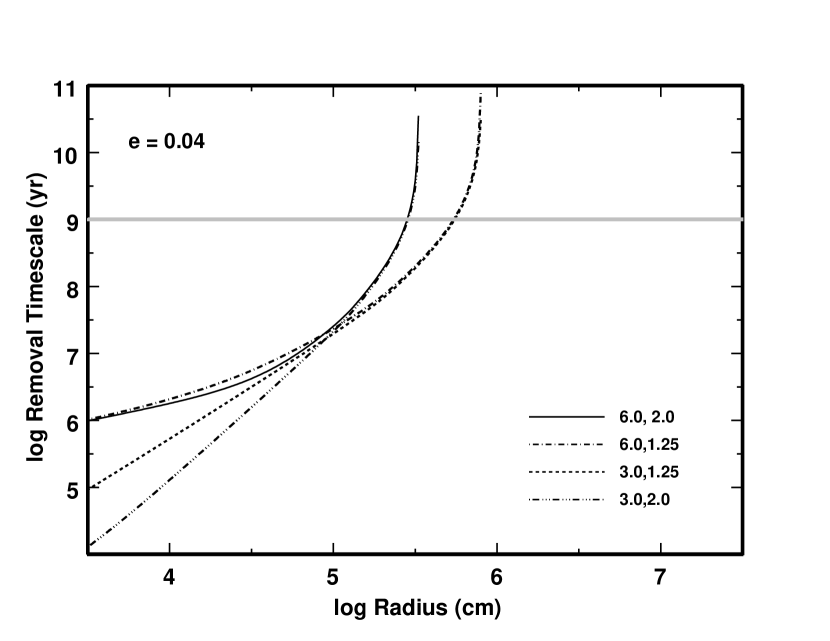
Figure 2: Removal timescale as a function of size for KBO collisions with $e$ = 0.04. The legend lists log $Q_{b}$ and $\beta_{g}$ for each curve.

Figure 2 plots several realizations of the analytic model as a function of KBO radius for a model with a mass equal to the minimum mass solar nebula and fragmentation parameters listed in the legend. For any combination of $Q_{b}$ and $\beta_{g}$, the removal timescale $t_{r}$ is a strong function of the KBO radius. Small KBOs with $r\leq$ 1 km have large $\dot{m_{l}}/m_{0}$ and small removal timescales of 1 Myr or less. Larger objects lose a smaller fraction of their initial mass per unit time and have $t_{r}\sim$ 1–1000 Gyr. KBOs with smaller $\beta_{g}$ are more easily disrupted and have smaller disruption times than KBOs with larger $\beta_{g}$.

Figure 2 also illustrates the derivation of the break radius, $r_{b}$. The horizontal line at $t$ = 1 Gyr intersects the model curves at $r_{b}\sim$ 3 km ($\beta_{g}$ = 2) and at $r_{b}\sim$ 6 km ($\beta_{g}$ = 1.25). The break radius is clearly independent of the bulk strength $Q_{b}$, and the reference time $t_{0}$, but is sensitive to $\beta_{g}$ and $e$. At fixed collision energy, KBOs with smaller $\beta_{g}$ fragment more easily. Thus, the break radius becomes larger as $\beta_{g}$ becomes smaller. At fixed strength, KBOs with larger impact velocities also fragment more easily. Thus, the break radius becomes larger with larger $e$.

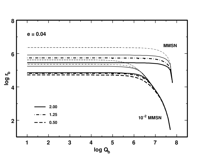
Figure 3: Break radius, $r_{b}$, as a function of the bulk strength, log $Q_{b}$, for collisions with $e$ = 0.04. The legend lists $\beta_{g}$ for each curve. Heavy lines have $C_{g}=2.25\times 10^{5(1.25-\beta_{g})}$ erg g^-1; light lines have $C_{g}=0.225\times 10^{5(1.25-\beta_{g})}$ erg g^-1. The upper set of curves plots results for a minimum mass solar nebula; the lower set plots results for models with 1% of the mass in a minimum mass solar nebula.

As in Pan & Sari (2004), the break radius depends on the initial mass in KBOs and the collision velocity. For classical KBOs with $e\approx$ 0.04, the break radius is $r_{b}\lesssim$ 10–20 km when $M_{KBO}\lesssim$ 10 $M_{\oplus}$ (Figure 3). In our model, $r_{b}$ grows with the initial mass in KBOs. We derive roughly an order of magnitude change in $r_{b}$ for a two order of magnitude change in the initial mass in KBOs.

The break radius is also sensitive to $C_{g}$ and $\beta_{g}$. KBOs with small $C_{g}$ and $\beta_{g}$ are easier to fragment than KBOs with large $C_{g}$ and $\beta_{g}$. For a fixed mass in KBOs, plausible variations in $C_{g}$ and $\beta_{g}$ yield order of magnitude variations in $r_{b}$ (Figure 3). At large $Q_{b}$, these differences disappear. For a Kuiper Belt with 1% of the mass in a minimum mass solar nebula, the model predicts no dependence of $r_{b}$ on the physical variables for $Q_{b}\gtrsim 3\times 10^{6}$ erg g^-1. This limit lies at $Q_{b}$ $\gtrsim 10^{8}$ erg g^-1 for a minimum mass solar nebula.

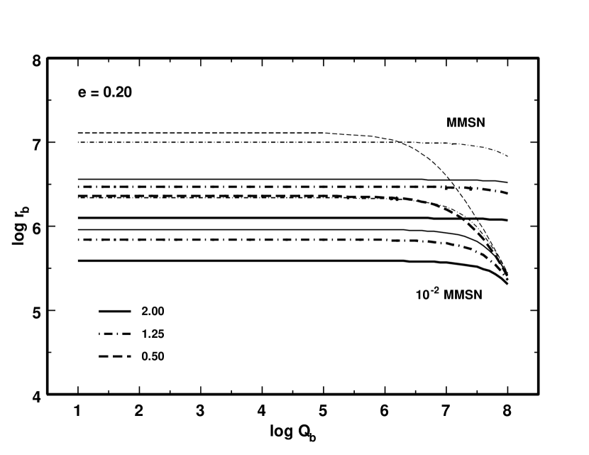
Figure 4: As in Figure 4, for $e$ = 0.2.

Figure 4 shows how changes in the collision energy modify $r_{b}$. Models with large eccentricity, $e$ = 0.20, yield $r_{b}\approx$ 3–100 km, compared to 0.3–10 km for $e$ = 0.04. The predicted $r_{b}$ is sensitive to the initial mass in KBOs, but is less sensitive to $C_{g}$ and $\beta_{g}$.

In contrast to Pan & Sari (2004), our analytic model indicates that a large break radius does not require a small bulk strength for the planetesimals. When the initial mass in KBOs is small, $\sim$ 1% to 10% of the minimum mass solar nebula, the collision frequency for 10–100 km KBOs is also small, $\sim$ 10–100 Gyr^-1. To remove sufficient material in 5 Gyr, these collisions must produce mostly debris. Thus, $Q_{d}$ must be small. Large bulk strengths, $Q_{b}\gtrsim 10^{6}$ erg g^-1, preclude debris-producing collisions (Figure 1) and result in small $r_{b}$ (Figures 3–4). As the initial mass in KBOs increases to 10% to 100% of the minimum mass solar nebula, collision frequencies also increase. More frequent collisions can remove large KBOs from the size distribution even when $Q_{b}$ is large. Thus, the break radius is less sensitive to $Q_{b}$ for massive nebulae.

2.3 Implications for the Kuiper Belt

The conclusions derived from the analytic model have direct implications for the formation and evolution of KBOs. The apparent break in the sky surface density at $R\approx$ 28 requires a break in the size distribution at $r_{b}\approx$ 20 km for an albedo of 0.04. The analytic model shows that a measured $r_{b}\gtrsim$ 20 km requires a nebula with a mass in solids of at least 10% of the minimum mass solar nebula. Producing such a large break radius from collisions is easier in an initially more massive nebula. The current mass in KBOs is $\lesssim$ 1% of the minimum mass solar nebula. Thus, the analytic model provides additional support for an initially more massive solar nebula at 30–50 AU (see also Stern & Colwell, 1997a; Kenyon & Luu, 1999a; Kenyon, 2002, and references therein).

The break in the sky surface density also favors a low bulk strength, $Q_{b}\lesssim 10^{6}$ erg g^-1, for KBOs. This $Q_{b}$ is smaller than the $Q_{b}\approx 10^{7}$ erg g^-1 derived from numerical models of collisions of icy bodies (e.g., Benz & Asphaug, 1999). However, a low bulk strength is consistent with the need for a strengthless rubble pile in models of the break-up of comet Shoemaker-Levy 9 (e.g., Asphaug & Benz, 1996).

The analytic model may also explain differences in the observed size distributions for different dynamical classes of KBOs. From Figures 3–4, resonant KBOs and scattered KBOs with large $e$ and $i$ should have a larger $r_{b}$ than classical KBOs with small $e$ but large $i$ (Luu & Jewitt, 2002). The group of ‘cold’ classical KBOs with small $e$ and small $i$ (Levison & Stern, 2001) should have even smaller $r_{b}$. The observations provide some support for this division. Relative to the number of bright KBOs, there are fewer faint resonant and scattered KBOs and more classical KBOs than expected (Bernstein et al., 2003). Long-term collisional evolution could be responsible for removing higher velocity resonant and scattered KBOs and leaving behind lower velocity classical KBOs.

To test the analytic model and provide direct comparisons with the observations, we need a numerical model of accretion and erosion. A numerical model accurately accounts for the time dependence of the total mass in KBOs and thus provides a clear measure of the removal time for a range of sizes. Numerical models also yield a direct calculation of the size distribution and thus measure the ‘depletion’ of KBOs as a function of radius.

3 NUMERICAL MODELS

To test the analytic model, we examine numerical simulations with a multiannulus coagulation code (Kenyon & Bromley, 2004, and references therein). For a set of $N$ concentric annuli surrounding a star of mass $M$, this code solves numerically the coagulation and Fokker-Planck equations for bodies undergoing inelastic collisions, drag forces, and long-range gravitational interactions (Kenyon & Bromley, 2002). We adopt collision rates from kinetic theory and use an energy-scaling algorithm to assign collision outcomes (Davis et al., 1985; Wetherill & Stewart, 1993; Weidenschilling et al., 1997; Benz & Asphaug, 1999). We derive changes in orbital parameters from gas drag, dynamical friction, and viscous stirring (Adachi et al., 1976; Ohtsuki, Stewart, & Ida, 2002). The appendix describes updates to algorithms described in Kenyon & Bromley (2001, 2002a, 2004) and Kenyon & Luu (1998, 1999).

We consider two sets of calculations. For models without gravitational stirring, we set $e$ = constant, $i$ = $e$/2, and calculate the collisional evolution of an initial power law size distribution. These calculations require a relatively small amount of computer time and allow a simple test of the analytic model.

Complete evolutionary calculations with collisional evolution and gravitational stirring test whether particular outcomes are physically realizable. These models also provide direct tests with observables, such as the current mass in KBOs and the complete KBO size distribution. Because these models do not allow arbitrary $e$ and $i$, they are less flexible than the constant $e$ models.

To provide some flexibility in models with gravitational stirring, we calculated models with and without stirring by Neptune at 30 AU. In models without Neptune, large KBOs with radii of 1000–3000 km stir up smaller KBOs to the disruption velocity. The KBO size distribution, including the break radius, then depends on the radius of the largest KBO $r_{L,KBO}$ formed during the calculation. Because $r_{L,KBO}$ depends on $Q_{b}$ and $Q_{g}$ (e.g., Kenyon & Luu, 1999a; Kenyon, 2002), $r_{b}$ also depends on $Q_{b}$ and $Q_{g}$.

In models with Neptune, long-range stirring by Neptune can dominate stirring by local large KBOs. The break radius then depends on the long-range stirring formula (Weidenschilling, 1989; Ohtsuki, Stewart, & Ida, 2002) and the timescale for Neptune formation. Here, we assume a 100 Myr formation time for Neptune, whose semimajor axis is fixed at 30 AU throughout the calculation. The mass of Neptune grows with time as

$$M_{Nep}\approx\left\{\begin{array}[]{l l l}6\times 10^{27}~{}e^{(t-t_{0})/t_{1}}~{}{\rm g}&&t<t_{0}\\ \\ 6\times 10^{27}~{}{\rm g}~{}+~{}C_{Nep}(t-t_{1})&&t_{0}<t<t_{2}\\ \\ 1.0335\times 10^{29}~{}{\rm g}&&t>t_{2}\\ \end{array}\right.$$ (13)

where $C_{Nep}$ is a constant and $t_{0}$, $t_{1}$, and $t_{2}$ are reference times. For most calculations, we set $t_{0}$ = 50 Myr, $t_{1}$ = 3 Myr, and $t_{2}$ = 100 Myr. These choices allow our model Neptune to reach 1 $M_{\oplus}$ in 50 Myr, when the largest KBOs have formed at 40–50 AU, and reach its current mass in 100 Myr. This prescription is not intended as a model for Neptune formation, but it provides sufficient extra stirring to test the prediction that the break radius depends on the amount of local stirring.

3.1 Constant eccentricity models

Calculations with constant eccentricity allow a direct test of the analytic model. We performed a suite of $\sim$ 200 4.5 Gyr calculations for a range in fragmentation parameters, with log $Q_{b}$ = 1–8, $\beta_{g}$ = 0.5–2.0, and log $C_{g}$ + 5 $\beta_{g}$ = 0.01–20. The initial size distribution of icy planetesimals has sizes of 1 m to 100 km in mass bins with $\delta=m_{i+1}/m_{i}$ = 1.7 and equal mass per mass bin. The planetesimals lie in 32 annuli extending from 40 AU to 75 AU. The central star has a mass of 1 M_⊙. The initial surface density, $\Sigma_{0}=10^{-3}$ g cm^-2 to $10^{-1}$ g cm^-2 at 40 AU, ranges from 1% to 100% of the minimum mass solar nebula extended to the Kuiper Belt (Weidenschilling, 1977; Hayashi, 1981). The initial eccentricity, $e$ = 0.04 and 0.20, spans the observed range for classical and resonant KBOs (Luu & Jewitt, 2002).

In Kuiper Belt models with large $e$, fragmentation is the dominant physical process (see also Stern & Colwell, 1997a; Kenyon & Luu, 1999a; Kenyon & Bromley, 2002). Large, 10–100 km objects grow very slowly. Smaller objects suffer numerous disruptive collisions that produce copious amounts of debris. Debris fills lower mass bins, which suffer more disruptive collisions. In 10–100 Myr, this collisional cascade reduces the population of 0.1–1 km and smaller objects. The size distribution then follows a broken power law, with $\alpha_{L}\approx$ 3 for large objects and $\alpha_{S}\approx$ 2.5 for the small objects (Dohnanyi, 1969; Williams & Wetherill, 1994; Pan & Sari, 2004).

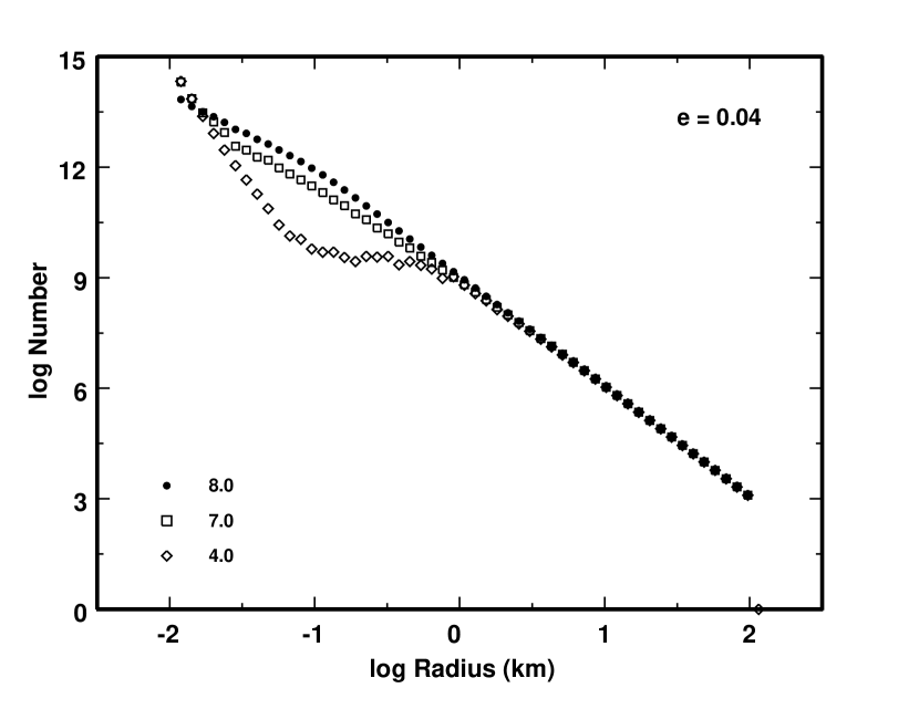
Figure 5: Size distributions at 4.5 Gyr for numerical models with constant $e$ = 0.04. The legend lists log $Q_{b}$ for each model.

As the evolution proceeds, the size distribution evolves into a standard shape (Figure 5). After 4.5 Gyr, the largest objects grow from 100 km to 125 km. From $\sim$ 10 km to 125 km, the size distribution continues to follow a power-law with $\alpha_{L}\approx$ 3. Test calculations suggest that this power law slope is fairly independent of the initial power law.

At smaller sizes, the shape of the size distribution depends on the bulk strength. For $Q_{b}\gtrsim 10^{6}$ erg g^-1, disruptive collisions produce a break in the size distribution; the power law slope changes from $\alpha_{L}\approx$ 3 to $\alpha_{S}\approx$ 2.5. For $Q_{b}\lesssim 10^{4}$ erg g^-1, disruptive collisions produce two breaks, one at 1–10 km and another at $\sim$ 0.1 km (Figure 5). The break at 1–10 km is where growth by accretion roughly balances loss by disruption. The break at $\sim$ 0.1 km is where debris produced by collisions of larger objects roughly balances loss by disruptive collisions. Between these two sizes, the slope of the size distribution ranges from $\alpha_{I}\approx-0.5$ for $Q_{b}\sim 10$ erg g^-1 to $\alpha_{I}\approx 1$ for $Q_{b}\sim 10^{5}$ erg g^-1. The slope of the power law for small sizes ranges from $\alpha_{I}\approx$ 4.5–5.0 for $Q_{b}\sim 10$ erg g^-1 to $\alpha_{I}\approx$ 3 for $Q_{b}\sim 10^{5}$ erg g^-1. As $Q_{b}$ approaches $10^{6}$ erg g^-1, the slopes of both power laws converge to $\alpha\approx$ 2.5.

We define the first inflection point in the size distribution as the break radius. To measure $r_{b}$, we use a least-squares fit to derive the best-fitting power-law slopes, $\alpha_{L}$ and $\alpha_{I}$, to the calculated size distribution. Using Poisson statistics to estimate errors in $N$, we derive $r_{b}$ and its 1$\sigma$ error by minimizing the residuals in the fits. Typical errors in log $r_{b}$ are $\pm$ 0.02-0.05. Tests indicate that the derived $r_{b}$ is more sensitive to the mass resolution of our calculations, $\delta$, than to the range in log $r$ used in the fits. This error is also small compared to the range in log $r_{b}$, $\sim$ 0.2, derived from repeat calculations with the same combination of $Q_{b}$ and $\beta_{g}$.

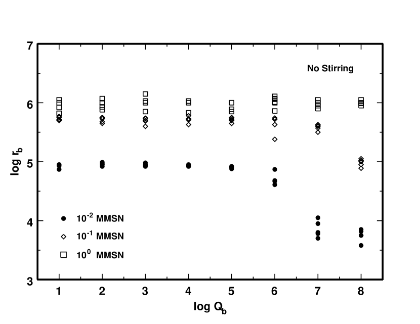
Figure 6: Variation of $r_{b}$ with $Q_{b}$ for numerical calculations at 40-47 AU with constant $e$=0.04. The legend indicates the initial mass in solids for each set of calculations.

Figure 6 shows results for calculations with constant $e$ = 0.04. For all initial masses and $Q_{b}\lesssim 10^{6}$, $r_{b}$ is independent of $Q_{b}$. For small initial masses, calculations with stronger objects yield small break radii. At larger initial masses, this sensitivity to $Q_{b}$ disappears. Calculations for minimum mass solar nebulae show little variation of $r_{b}$ with $Q_{b}$.

These results confirm the basic features of the analytic model. Both models predict $r_{b}\lesssim$ 1 km for low mass nebulae with $\sim$ 1% of the mass in the minimum mass solar nebula. Larger break radii, $\sim$ 1–10 km, are possible in more massive nebulae. The analytic model predicts large break radii for larger $e$ than the numerical calculations. In numerical calculations with $e$ = 0.2, disruptive collisions reduce the space density considerably in $\sim$ 100 Myr. The smaller collision rates prevent formation of a break in the size distribution at large radii. Thus, numerical calculations with $e$ = 0.2 yield log $r_{b}$ only $\sim$ 0.1–0.2 larger than calculations with $e$ = 0.04.

3.2 Full evolution models

These calculations begin with 1–1000 m planetesimals in mass bins with $\delta$ = 1.4 or 1.7 and equal mass per bin. The planetesimals lie in 32 annuli at 40–75 AU. Models with Neptune have an extra annulus at 30 AU. For most models, we adopt $e_{0}=10^{-4}$ or $e_{0}$ = $10^{-5}$ and $i$ = $e$/2 for all planetesimals. At the start of our calculations, these initial values yield a rough balance between viscous stirring by 0.1–1 km objects and collisional damping of 10–100 m objects. The bodies have a mass density $\rho_{d}$ = 1.5 g cm^-3, which is fixed throughout the evolution. We consider a range in initial surface density, with $\Sigma_{0}$ = 0.03–0.3 g cm^-2 ($a_{0}$/30 AU)^-3/2.

To measure the sensitivity of our results to stochastic variations, we performed 2–5 calculations for each set of fragmentation parameters. For $\beta_{b}$ = 0 and a factor of ten range in $\Sigma_{0}$, we considered log $Q_{b}$ = 1, 2, 3, 4, 5, 6, and 7; $C_{0}$ = 0.15 and 1.5; and $\beta_{g}$ = 1.25 and 2.0. We also performed a limited set of calculations for $C_{g}$ = 0.15 and 1.5, $\beta_{g}$ = 0.5, and a small set of log $Q_{b}$. Although stochastic variations can change the size of the largest object at 40–50 AU, repeat calculations with identical initial conditions yield small changes in the shape of the size distribution or the location of the break radius. A few calculations with $\beta_{b}\neq$ 0 yield interesting behavior in the size distribution at 1–100 m sizes, but $r_{b}$ does not change dramatically. A larger suite of calculations with $\beta_{v}\neq$ 0 leads to similar conclusions. We plan to report on these aspects of the calculations in a separate paper.

Icy planet formation in the outer solar system follows a standard pattern (see Kenyon & Luu, 1999a; Kenyon & Bromley, 2004; Goldreich, Lithwick, & Sari, 2004). Small planetesimals with $r_{i}\lesssim$ 1 km first grow slowly. Collisonal damping brakes the smallest objects. Dynamical friction brakes the largest objects and stirs up the smallest objects. Gravitational focusing factors increase, and runaway growth begins. At 40–50 AU, it takes $\sim$ 1 Myr to produce 10 km objects and another 3–5 Myr to produce 100 km objects. Continued stirring reduces gravitational focusing factors. Collisions between the leftover planetesimals produce debris instead of mergers. Runaway growth ends and the collisional cascade begins.

During the collisional cascade, the mass in 1–10 km and smaller objects declines precipitously. Because gravitational focusing factors are small, collisions between two planetesimals are more likely than collisions between a planetesimal and a 100–1000 km protoplanet. Thus, disruptive collisions grind leftover planetesimals into small dust grains, which are removed by radiation pressure and Poynting-Robertson drag (e.g., Burns, Lamy, & Soter, 1979; Takeuchi & Artymowicz, 2001). At 40–50 AU, the surface density falls by a factor of two in 100–200 Myr, a factor of 4–5 in 1 Gyr, and more than an order of magnitude in 3–4 Gyr (see also Kenyon & Bromley, 2004). After 4.5 Gyr, the typical amount of solid material remaining at 40–50 AU is 3% to 10% of the initial mass (see below).

As collisions and radiation remove material from the system, the largest objects continue to grow slowly. In most calculations, it takes 10–50 Myr to produce the first 1000 km object. The largest objects then double their mass every 100 Myr to 1 Gyr. After 4.5 Gyr, the largest objects have radii ranging from $\sim$ 100 km ($Q_{b}\lesssim 10^{3}$ erg g^-1, $\beta_{g}$ = 0.5) to 5000 km ($Q_{b}\gtrsim$ $10^{7}$ erg g^-1, $\beta_{g}$ = 2.0). Calculations with $\beta_{g}$ = 1.25 and $Q_{b}\sim 10^{2}$ erg g^-1 to $10^{4}$ erg g^-1 favor the production of objects with radii of 1000–2000 km, as observed in the outer solar system.

These general results are remarkably independent of the initial conditions and of some input parameters (Kenyon & Luu, 1999a; Kenyon & Bromley, 2004). The size distribution of objects remaining at 4.5 Gyr is not sensitive to the initial disk mass, the initial size distribution, the initial eccentricity and inclination (for $e_{0}\lesssim 10^{-3}$), the mass resolution $\delta$, the width of an annulus $\delta a$, or the gas drag parameters. The orbital period $P$ and the surface density set the collision timescale, $t\propto P/\Sigma$. Although stochastic variations can produce factor of 2 or smaller variations in growth times, all timescales depend on the collision time and scale with the current surface density.

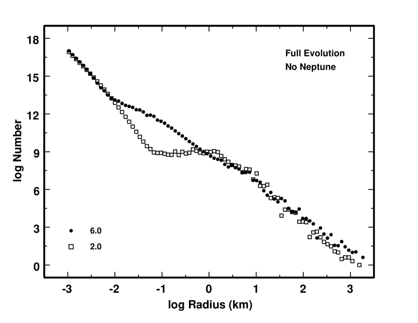
Figure 7: Size distributions at 4.5 Gyr for complete numerical models of KBO evolution at 40–47 AU. The legend lists log $Q_{b}$ for each model.

To derive $r_{b}$ for these calculations, we again examine the size distribution at 4.5 Gyr (Figure 7). For radii $r_{i}\sim$ 10–1000 km, the size distribution follows a power-law, $N\propto r^{-\alpha_{L}}$ with slope $\alpha_{L}\approx$ 3–3.5. For smaller radii, the size distribution has inflection points at log $r_{i}\approx$ $-$1 to 1 and at log $r_{i}\lesssim$ $-$1. Between the two inflection points, the power-law slope is shallow, with $\alpha_{I}\approx$ 0–2. For small objects, the power-law slope is steep, with $\alpha_{S}\approx$ 2–4.

The slope of the intermediate power-law depends on the fragmentation parameters. Calculations with small $Q_{b}$ and $\beta_{g}$ yield small $\alpha_{I}$. For larger $Q_{b}$ and $\beta_{g}$, the slope approaches the collisional limit, $\alpha_{I}\approx$ 2.5 (Dohnanyi, 1969; Williams & Wetherill, 1994). The extent of the shallow, intermediate power-law also varies with $Q_{b}$ and $\beta_{g}$. For $Q_{b}\lesssim 10^{3}$ erg g^-1 and $\beta_{g}\approx$ 1.25, the size distribution is relatively flat from log $r_{i}\approx$ $-1$ to 0.0–0.5 (Figure 7). Large $Q_{b}$ and $\beta_{g}$ result in a smaller extent for the intermediate power law.

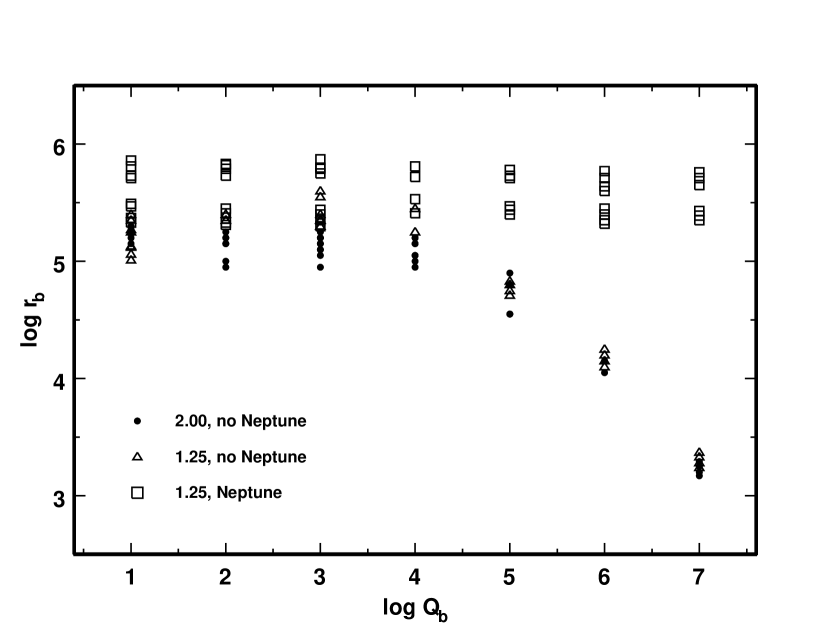
Figure 8: Variation of $r_{b}$ with $Q_{b}$ for complete numerical calculations of KBO evolution at 40-47 AU. All calculation begin with a mass in solids equivalent ot the minimum mass solar nebula. The legend indicates log $Q_{b}$ for each set of models. Calculations with Neptune use a simple model for the growth of Neptune at 30 AU.

Figure 8 shows results for $r_{b}$ as a function of log $Q_{b}$ for several sets of calculations. All calculations began with a mass in solids comparable to a minimum mass solar nebula. For models without stirring by Neptune, we derive log $r_{b}\approx$ 5.0–5.6 (log $Q_{b}\lesssim$ 4) and log $r_{b}\approx$ $5.3\pm 0.3-0.5$ log $Q_{b}$ (log $Q_{b}\gtrsim$ 4). Although there is some overlap in the results for different sets of parameters, a weaker gravity component to the disruption energy ($\beta_{g}\approx$ 1.25) favors larger $r_{b}$. This result confirms the conclusion derived from the analytic model.

Stirring by Neptune yields larger values for the break radius (Figure 8). As Neptune reaches its final mass at 80–100 Myr, long-range stirring rapidly increases the eccentricities of objects at 40–50 AU. This stirring accelerates the collisional cascade, which depletes the population of small planetesimals and halts the growth of the largest objects. The larger $e$ and longer duration of the collisional cascade moves the break in the size distribution to larger radii.

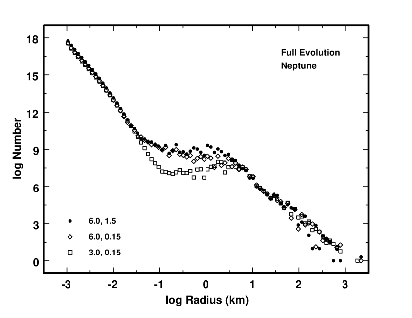
Figure 9: As in Figure 7, for models with Neptune at 30 AU.

Figure 9 shows size distributions at 4.5 Gyr for three models with stirring by Neptune. The legend lists input values for $Q_{g}$ and log $Q_{b}$. In these calculations, the break is at $r_{b}\approx$ 5–10 km, compared to $r_{b}\approx$ 1–5 km for models without Neptune stirring. The position of the break is relatively independent of $Q_{b}$ or $Q_{g}$ (see Figure 8). For KBOs with sizes smaller than the break, the slope of the size distribution is sensitive to $Q_{b}$ but not to $Q_{g}$. Models with $Q_{b}\gtrsim 10^{4}$ erg g^-1 have more small objects with radii of $\sim$ 0.1 km than models with $Q_{b}\lesssim 10^{4}$ erg g^-1.

3.3 Comparisons with observations of KBOs

The analytic model and the numerical evolution calculations yield a consistent picture for the size distribution of icy bodies in the outer solar system. The general shape of the size distribution does not depend on the initial conditions or input parameters. The typical size distribution has two power laws – one power-law for large objects with radii $\gtrsim$ 10–100 km and a second power-law for small objects with radii $\lesssim$ 0.1 km – connected by a transition region where the number of objects per logarithmic mass bin is roughly constant. The power law slope for the large objects is also remarkably independent of input parameters and initial conditions.

The fragmentation parameters and the amount of stirring set the location of the transition region and the power-law slope for the small objects. In our calculations, the break radius is $r_{b}\gtrsim$ 10 km when icy objects are easy to break and the stirring is large. Strong icy objects and small stirring favor a small break radius, $r_{b}\lesssim$ 1 km. When the break radius is small, the extent of the transition region is also small, less than an order of magnitude in radius. When the break radius is large, the transition region can extend for 2 orders of magnitude in radius.

To compare the numerical results to observations of KBOs, we convert a calculated size distribution into a predicted sky surface density of KBOs as a function of apparent magnitude. Current observations suggest that the observed sky surface density, $\sigma(m)$ – the number of KBOs per square degree on the sky, follows a power law

$${\rm log}~{}\sigma(m)={\rm log}~{}\sigma_{0}+\alpha(m-m_{0})$$ (14)

where $\alpha$, $\sigma_{0}$ and $m_{0}$ are constants. With $\alpha\approx$ 0.6 and $m_{0}$ = 23, this function fits the data fairly well for R-band magnitudes, $R\approx$ 22–26. For $R\lesssim$ 22 and $R\gtrsim$ 26, the simple function predicts too many KBOs compared to observations (Bernstein et al., 2003). The observations also suggest that the scattered and Plutino populations of KBOs have different surface density distributions than classical KBOs, with $\alpha\approx$ 0.6 for scattered KBOs and Plutinos and $\alpha\approx$ 0.8 for classical KBOs (Bernstein et al., 2003).

Because we do not include the dynamics of individual objects in our calculations, we cannot predict the relative numbers of KBOs in different dynamical classes. However, we can predict $\sigma(m)$ for all KBOs and see whether the calculations can explain trends in the observations.

To derive a model $\sigma(m)$, we assign distances $d_{\odot}$ to an ensemble of objects chosen randomly from the model size distribution. For a random phase angle $\beta$ between the line-of-sight from the Earth to the object and the line-of-sight from the Sun to the object, the distance of the object from the Earth is $d_{E}=d_{\odot}{\rm cos}\beta-(1+d_{\odot}^{2}({\rm cos}^{2}\beta-1))^{1/2}$. The red magnitude of this object is $R=R_{0}+2.5~{}{\rm log}~{}(t_{1}/t_{2})-5~{}{\rm log}~{}r_{KBO}$, where $R_{0}$ is the zero point of the magnitude scale, $r_{i}$ is the radius of the object, $t_{1}=2d_{\odot}d_{E}$, and $t_{2}=\omega((1-g)\phi_{1}+g\phi_{2})$ (Bowell et al., 1989). In this last expression, $\omega$ is the albedo, and $g$ is the slope parameter; $\phi_{1}$ and $\phi_{2}$ are phase functions that describe the visibility of the illuminated hemisphere of the object as a function of $\beta$. We adopt standard values, $\omega=0.04$ and $g=0.15$, appropriate for comet nuclei (Jewitt et al., 1998; Luu & Jewitt, 2002; Brown & Trujillo, 2004). The zero point $R_{0}$ is the apparent red magnitude of the Sun, $m_{R,\odot}$ = $-$27.11, with a correction for the V–R color of a KBO, $R_{0}$ = $m_{R,\odot}$ + $\delta$(V–R)_KBO. Observations suggest that KBOs have colors that range from roughly $-0.1$ to 0.3 mag redder than the Sun (Jewitt & Luu, 2001; Tegler & Romanishin, 2003; Tegler, Romanishin, & Consolmagno, 2003). We treat this observation by allowing the color to vary randomly in this range.

For this application, we assign distances $d_{\odot}$ = 40–50 AU and derive the number of objects in half magnitude bins for $R$ = 15–50. In most models, the surface density of objects predicted by the model closely follows the linear relation for log $\sigma$ with $\alpha\approx$ 0.55–0.7 and $R_{0}\approx$ 21–24 (see also Kenyon & Luu, 1999b; Kenyon, 2002). To make easier comparisons between observations and theory, we follow Bernstein et al. (2003) and define the relative space density as the ratio between the model and the linear surface density relation with $\alpha$ = 0.6 and $R_{0}$ = 23.

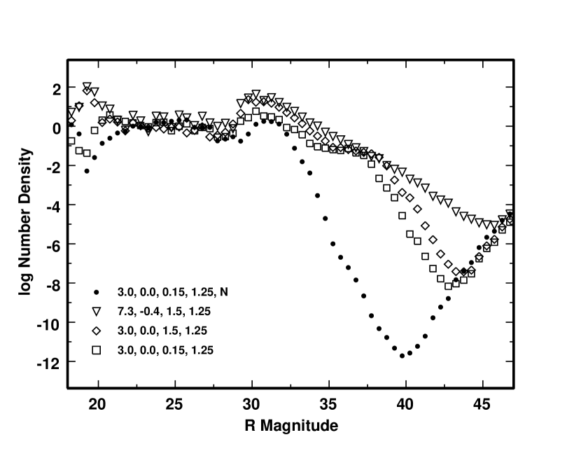
Figure 10: KBO luminosity functions derived from the planet formation model. The legend indicates fragmentation models for each model; the model with ‘N’ has Neptune stirring.

Figure 10 shows the relative surface density for several KBO calculations. For bright KBOs with $R\approx$ 22–28, the surface density closely follows the linear relation, equation (14). This result is independent of the fragmentation parameters, the initial mass at 40–50 AU, the initial size distribution, and the amount of stirring by Neptune. Thus, the coagulation models provide a robust prediction for $\alpha$ at $R\approx$ 22–28 (see also Kenyon & Luu, 1999b; Kenyon, 2002).

There are significant differences between the models at $R\lesssim$ 22 and $R\gtrsim$ 28. For $R\lesssim$ 22, the models fall into two broad classes defined by the ratio of the disruption energy to the typical collision energy, $Q_{d}/Q_{I}$. Calculations with large $Q_{d}/Q_{I}$ produce many large, bright KBOs. Calculations with small $Q_{d}/Q_{I}$ produce few large, bright KBOs. The range in production rates is roughly 4 orders of magnitude.

For fainter KBOs, the differences between models become even more significant. At $R\approx$ 27–30, collisions remove weak KBOs from the size distribution. Thus, most calculations with Neptune stirring exhibit a drop in the relative surface density. Calculations with $Q_{b}\lesssim 10^{3}$ erg g^-1, $Q_{g}\lesssim$ 0.1–0.2, and no Neptune stirring also produce fewer KBOs at $R\approx$ 27–30.

Relative to the nominal power-law, all calculations produce an excess of KBOs at $R\approx$ 29–33. For weak KBOs with $Q_{b}\lesssim 10^{3}$ erg g^-1, the model predicts a factor of 3 excess compared to the power-law. For strong KBOs with $Q_{b}\gtrsim 10^{6}$ erg g^-1, this excess grows to a factor of 10–30. Stirring by Neptune has little impact on this excess.

For fainter KBOs with $R\gtrsim$ 32, stirring by Neptune is very important. Our models produce a 5–12 order of magnitude deficit of KBOs relative to the power-law surface density relation. Weaker KBOs produce larger deficits. Neptune stirring also produces larger deficits. We derive the largest deficit, 12 orders of magnitude at $R\approx$ 40, for models with Neptune stirring, $Q_{b}\lesssim 10^{4}$ erg g^-1, and $Q_{g}\lesssim$ 0.15 erg g^-1 (Figure 10).

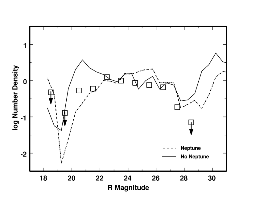
Figure 11: As in Figure 10, with observations of KBOs added for comparison (Bernstein et al., 2003).

The derived $\sigma(m)$ yields good agreement with the observations (Figure 11). For $R\approx$ 22–28, most models account for the variation of relative number density with R magnitude. Calculations with weaker KBOs, $Q_{b}\lesssim 10^{4}$ erg g^-1, reproduce the dip in the relative number density at $R\approx$ 19–20. Our ensemble of models suggests that the magnitude of the dip depends more on stochastic phenomena than on model parameters. The small $Q_{b}$ models also provide better agreement with observations for fainter KBOs with $R\approx$ 26–28. At $R\approx$ 20–21 and at $R\approx$ 29–30, models without Neptune stirring produce an excess of KBOs relative to the observations; models with Neptune stirring yield better agreement with the data. Thus, models with weak KBOs, $Q_{b}\lesssim 10^{4}$ erg g^-1, and with Neptune stirring provide the best explanation for current observations of the shape of the size distribution of KBOs.

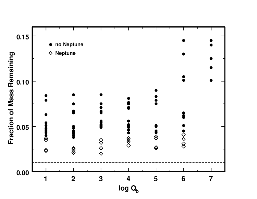
Figure 12: Fraction of initial mass remaining in complete KBO models at 4.5 Gyr. Filled circles: models without Neptune. Open circles: models with Neptune at 30 AU. At the bottom of the plot, the horizontal dashed line indicates the ratio of the current mass in the Kuiper Belt to the mass in solids of a minimum mass solar nebula.

In addition to the relative size distribution, the collision models provide fair agreement with the absolute numbers of KBOs (Figure 12). Current data suggest a total mass of $\sim$ 0.1 $M_{\oplus}$ in KBOs at 35–50 AU (Luu & Jewitt, 2002; Bernstein et al., 2003). To form KBOs by coagulation in 10–100 Myr, collision models require an initial mass in solids comparable to the minimum mass solar nebula. This result suggests that the current mass in KBOs is $\sim$ 1% of the initial mass in solid material at 35–50 AU. After 4.5 Gyr, our collision models have 3%–10% of the initial mass in 1 km and larger objects. Models with Neptune stirring are more efficient at removing material from the size distribution (Figure 12).

This result is encouraging. Once large objects form in the Kuiper Belt, the collisional cascade can remove almost all of the leftover planetesimals, which contain 90% to 97% of the initial mass (see also Stern & Colwell, 1997a; Kenyon & Luu, 1999a). Other processes not included in our calculations will also remove large objects. Dynamical interactions with Neptune and other giant planets can remove 50% to 80% of the initial mass (Holman & Wisdom, 1993; Levison & Stern, 1995). Interactions with field stars can also remove KBOs (Ida et al., 2000). Including these processes in a more realistic collision calculation should bring the predicted number of KBOs into better agreement with observations. We plan to describe calculations testing the role of Neptune in the formation and evolution of the Kuiper Belt.

Although we cannot develop tests using data for KBO dynamical families, the models provide some insight into general trends of these observations. Because scattered KBOs and most resonant KBOs have had close dynamical interactions with Neptune, these objects probably formed closer to the Sun than classical KBOs. If Neptune stirring halted accretion in the Kuiper Belt, this difference in heliocentric distance can produce an observable difference in KBO sizes. For a formation timescale, $t\propto P/\Sigma\propto a^{3}$, KBOs at 45 AU take twice as long to form as KBOs at 35 AU. During the late stages of runaway growth, this difference in formation timescales leads to a factor of $\sim$ 2 difference in the maximum size of a KBO. Although the oligarchic growth phase erases this difference, significant stirring by Neptune during runaway growth might preserve the difference and lead to the apparent lack of large classical KBOs (formed at $\sim$ 45 AU) relative to resonant KBOs (formed at $\sim$ 35 AU). We plan additional numerical calculations to test this idea.

4 CONCLUSIONS AND SUMMARY

We have developed an analytic model for the formation of a break in the power law size distribution of KBOs in the outer solar system. For a mass in KBOs equivalent to the current mass at 40–50 AU and for $e$ = 0.04 orbits, the model predicts a break at a radius, $r_{b}\sim$ 0.1–1 km. For a massive Kuiper Belt with $e$ = 0.2, the break moves to $r_{b}\sim$ 10–100 km. These results agree with the model of Pan & Sari (2004).

In contrast to Pan & Sari (2004), our model predicts a smaller sensitivity to the bulk strength of KBOs. When the mass in KBOs is 1% of the minimum mass solar nebula, $r_{b}$ is independent of $Q_{b}$ for $Q_{b}\lesssim$ $10^{6}$ erg g^-1. For $Q_{b}\gtrsim$ $10^{6}$ erg g^-1, $r_{b}$ declines with increasing $Q_{b}$. As the total mass in KBOs increases, the break radius is less sensitive to $Q_{b}$. When the mass in KBOs is comparable to a minimum mass solar nebula, the analytic model suggests that $r_{b}$ is roughly constant for all reasonable $Q_{b}$.

To test the analytic model, we used a suite of numerical simulations. Constant eccentricity calculations, with no velocity evolution due to gravitational interactions, confirm the analytic results. For models with constant $e$ = 0.04–0.20, the break radius depends on $Q_{b}$ and the total mass in KBOs,

$$r_{br}\approx\left\{\begin{array}[]{l l l}1.0\left(\frac{e}{0.04}\right)^{1/2}\left(\frac{M_{KBO}}{M_{KBO,0}}\right)^{1/2}~{}{\rm km}&&Q_{b}\lesssim 10^{6}~{}{\rm erg~{}g^{-1}}\\ \\ 0.1\left(\frac{e}{0.04}\right)^{1/2}\left(\frac{M_{KBO}}{M_{KBO,0}}\right)~{}{\rm km}&&Q_{b}\gtrsim 10^{7}~{}{\rm erg~{}g^{-1}}\\ \end{array}\right.$$ (15)

where $M_{KBO,0}$ is the mass of a minimum mass solar nebula extended into the Kuiper Belt, $\sim$ 10 $M_{\oplus}$ at 40–50 AU.

Simulations of complete KBO evolution, with velocity stirring, generally require more initial mass in planetesimals to yield the same results. In models without Neptune formation, stirring by large objects with radii of 1000–3000 km yield

$$r_{br}\approx\left\{\begin{array}[]{l l l}1-3~{}{\rm km}&&Q_{b}\lesssim 10^{4}~{}{\rm erg~{}g^{-1}}\\ \\ 1-3~{}\left(\frac{Q_{b}}{\rm 10^{4}~{}erg~{}g^{-1}}\right)^{1/2}~{}{\rm km}&&Q_{b}\gtrsim 10^{4}~{}{\rm erg~{}g^{-1}}\\ \end{array}\right.$$ (16)

for models starting with a mass in solid comparable to the minimum mass solar nebula. Calculations with Neptune at 30 AU allow larger break radii independent of $Q_{b}$, with

$$r_{br}\approx\begin{array}[]{l l l}3-10~{}{\rm km}&&Q_{b}\lesssim 10^{7}~{}{\rm erg~{}g^{-1}}\\ \end{array}$$ (17)

In both cases, models with more initial mass yield larger $r_{b}$.

Comparisons between observed and predicted size distributions of KBOs allow tests of models for KBO formation and evolution. For a broad range of input parameters, KBO models with and without stirring by Neptune yield good agreement with observations for $R\approx$ 21–27. The observed surface density of brighter KBOs suggests that KBOs have $Q_{b}\lesssim 10^{3}-10^{4}$ erg g^-1. Although stirring by Neptune modifies the shape of the KBO size distribution for $R\lesssim$ 22, the observations do not discriminate clearly between models with and without Neptune. Improved observational constraints on the surface density of KBOs for $R\lesssim$ 21–22 might provide tests for the relative formation times of Neptune and large KBOs.

Observations for $R\gtrsim$ 27 may also yield constraints on the formation of Neptune. Long-range stirring by Neptune is more important for the size distribution of fainter KBOs, $R\gtrsim$ 27. Most models predict a small dip in the size distribution at $R\approx$ 27–30, a peak at $R\approx$ 30–34, and a deep trough at $R\approx$ 35–45. Because stirring by Neptune removes more objects with radii of 1–30 km from the KBO size distribution, models with Neptune produce a larger dip and a deeper trough than models without Neptune. The depth of the small dip in models with Neptune stirring is close to the depth observed in recent HST observations (Bernstein et al., 2003).

Calculations with Neptune stirring yield many orders of magnitude fewer KBOs with $R\approx$ 32–42 than calculations without Neptune. Current observations do not probe this magnitude range. However, ongoing and proposed campaigns to detect small KBOs from occultations of background stars allow tests of the models (Bailey, 1976; Brown & Webster, 1997; Roques & Moncuquet, 2000; Cooray & Farmer, 2003; Roques et al., 2003). For $\omega$ = 0.04, detections of 1 km KBOs provide constraints at $R\approx$ 33–35, where Neptune stirring models predict a sharp drop in the KBO number density. Direct detections of smaller KBOs, with radii of $\sim$ 0.1 km, constrain model predictions at $R\approx$ 40, where Neptune stirring models predict 3–6 order of magnitude fewer KBOs than models without Neptune stirring.

After 4.5 Gyr of collisional evolution, all of the numerical calculations predict a small residual mass in large KBOs. For $Q_{b}\lesssim$ $10^{6}$ erg g^-1, the simulations leave $f\sim$ 3%-8% of the initial planetesimal mass in KBOs with radii of 1 km and larger. Models with stirring by Neptune contain less mass in KBOs than models without Neptune. Calculations with $Q_{b}\gtrsim$ $10^{6}$ erg g^-1 have a larger range in $f$; models with stirring by Neptune still leave $\sim$ 3%–5% of the initial mass in large KBOs.

These results are encouraging. Although our calculations leave more material in large objects than the current mass in KBOs, $\sim$ 0.5%–1% of a minimum mass solar nebula, other processes can reduce the KBO mass considerably. Formation of Neptune at 10–20 Myr, instead of our adopted 100 Myr, probably reduces our final mass estimates by a factor of two. Dynamical interactions with Neptune and passing stars can also remove substantial amounts of material (e.g., Holman & Wisdom, 1993; Levison & Stern, 1995; Duncan et al., 1995; Malhotra, 1996; Levison & Duncan, 1997; Morbidelli & Valsecchi, 1997; Ida et al., 2000). These studies suggest that a combination of collisional grinding and dynamical interactions with Neptune or a passing star can reduce a minimum mass solar nebula to the mass observed today in the Kuiper Belt. We plan to describe additional tests of these possibilities in future publications.

Finally, our calculations provide additional evidence that observations of Kuiper Belt objects probe the formation and early evolution of Neptune and other icy planets in the outer solar system. Better limits on the sizes of the largest KBOs probe the timescale for Neptune formation. These observations also constrain the bulk strength of KBOs during the formation epoch. The detection of small KBOs, $r\approx$ 0.1–10 km, by occultations (e.g. TAOS; Marshall et al., 2003) or by direct imaging (e.g., OWL; Gilmozzi, Rierckx, & Monnet, 2001) yields complementary constraints. As the observations improve, the theoretical challenge is to combine collisional (this paper; Goldreich, Lithwick, & Sari (2004)) and dynamical (e.g. Malhotra, 1995; Gomes, 2003; Levison & Morbidelli, 2003; Quillen, Trilling, & Blackman, 2004) calculations to derive robust predictions for the formation and evolution of Uranus, Neptune, and smaller icy planets at heliocentric distances $\gtrsim$ 15 AU. Together, the calculations and the observations promise detailed tests of theories of planet formation.

We acknowledge a generous allotment, $\sim$ 3000 cpu days from February 2003 through March 2004, of computer time at the supercomputing center at the Jet Propulsion Laboratory through funding from the NASA Offices of Mission to Planet Earth, Aeronautics, and Space Science. Advice and comments from M. Geller and S. A. Stern improved our presentation. We thank P. Michel and A. Morbidelli for extensive discussions that improved our treatment of collisional disruption. We also acknowledge discussions with P. Goldreich and M. Holman. The NASA Astrophysics Theory Program supported part of this project through grant NAG5-13278.

Appendix A APPENDIX

Kenyon & Luu (1998, 1999) and Kenyon & Bromley (2001, 2002a, 2004) describe algorithms and tests of our multiannulus planet formation code. Here, we describe an update to the fragmentation algorithm.

In previous calculations, we used fragmentation prescriptions summarized by Davis et al. (1985) and Wetherill & Stewart (1993). Both methods write the strength $S$ of a pair of colliding objects as the sum of a constant bulk strength, $S_{0}$, and the gravitational binding energy, $E_{g}$,

$$S=S_{0}+E_{g}~{}.$$ (A1)

For $E_{g}\propto(m_{i}+m_{j})/r_{ij}$, the strength is $S$ = $S_{0}$ + $S_{1}r_{ij}^{2}$, where $S_{1}$ is a constant and $r_{ij}$ is the radius of an object with mass $m_{i}+m_{j}$. When the collision energy, $Q_{I}$, exceeds $S$, Wetherill & Stewart (1993) derive the mass lost by catastrophic disruption as the ratio of the impact energy to a crushing energy $Q_{c}$. Davis et al. (1985) assume that a fixed fraction, $f_{KE}$, of the impact kinetic energy is transferred to ejected material and derive the fraction of the combined mass lost to disruption. In most cases, the Davis et al. (1985) algorithm yields less debris than the Wetherill & Stewart (1993) algorithm.

To take advantage of recent advances in numerical simulations of collisions (e.g., Benz & Asphaug, 1999; Michel et al., 2001, 2002, 2003), we now define a disruption energy $Q_{d}$ required to eject 50% of the combined mass of two colliding bodies (equation 3 in the main text). For collision energy $Q_{I}$, the mass ejected in a catastrophic collision is $m_{ej}=0.5(m_{1}+m_{2})(Q_{I}/Q_{d})^{\beta_{e}}$. For most applications we set $\beta_{e}$ = 1.125 (e.g., Davis et al., 1985). When $m_{ej}<10^{-8}$ $(m_{i}+m_{j})$, we follow Wetherill & Stewart (1993) and set $m_{ej}$ = 0.

To derive the size and velocity distribution of the ejected material, we adopt a simple procedure for all collisions. We define the remnant mass,

$$m_{rem}=m_{i}+m_{j}-m_{ej}~{}.$$ (A2)

The mass of the largest ejected body is

$$m_{L,ej}=0.2m_{ej}$$ (A3)

We adopt a cumulative size distribution for the remaining ejected bodies, $n_{c}(m)\propto m^{-b}$, with $b$ = 0.8 (Dohnanyi, 1969; Williams & Wetherill, 1994), and require that the mass integrated over the size distribution equal $m_{ej}$. We assume that all bodies receive the same kinetic energy per unit mass, given by the initial relative velocities of the two bodies,

$$V_{ij}^{2}=h_{i}^{2}+v_{i}^{2}+h_{j}^{2}+v_{j}^{2}~{},$$ (A4)

where $h$ and $v$ are the horizontal and vertical components of the velocity dispersion relative to a circular orbit (e.g. Kenyon & Luu, 1998). We derive mass-weighted $h_{i}^{\prime}$ and $v_{i}^{\prime}$ for the combined object and the debris, $V_{ij}^{2}$ = $(h_{i}^{\prime})^{2}$ + $(v_{i}^{\prime})^{2}$.

This procedure, which we apply to cratering and disruptive collisions, is computationally efficient and maintains the spirit of recent analytic models and numerical simulations. Comparisons with our previous results using the Davis et al. (1985) and Wetherill & Stewart (1993) algorithms suggest that the new algorithm yields intermediate ‘mass loss rates’ for $\beta_{g}$ = 2 and $Q_{b}\sim 10^{2}$–$10^{6}$ erg g^-1. Calculations with $\beta_{g}$ $\sim$ 1.2–1.5 (Benz & Asphaug, 1999) yield larger mass loss but do not change the results significantly. When the bulk strength depends on the particle radius, the size distribution for small objects with $r_{i}\lesssim$ 0.1 km depends on the exponent $\beta_{b}$ of the bulk component of the strength. We plan to report on the details of these differences in future papers on the formation of KBOs and terrestrial planets.

References

- (1)
- Adachi et al. (1976) Adachi, I., Hayashi, C., & Nakazawa, K. 1976, Progress of Theoretical Physics 56, 1756
- Allen et al. (2001) Allen, R. L., Bernstein, G. M., & Malhotra, R. 2001, ApJ, 549, L241
- Artymowicz (1997) Artymowicz, P. 1997, ARE&PS, 25, 175
- Asphaug & Benz (1996) Asphaug, E., & Benz, W. 1996, Icarus, 121, 225
- Backman & Paresce (1993) Backman, D. E., & Paresce, F. 1993, in Protostars and Planets III, ed. E. H. Levy & J. I. Lunine (Tucson: Univ of Arizona), p. 1253
- Backman, Dasgupta, & Stencel (1995) Backman, D. E., Dasgupta, A., & Stencel, R. E. 1995, ApJ, 450, L35
- Bailey (1976) Bailey, M. 1976, Nature, 259, 290
- Benz & Asphaug (1999) Benz, W., & Asphaug, E. 1999, Icarus, 142, 5
- Bernstein et al. (2003) Bernstein, G. M., Trilling, D. E., Allen, R. L., Brown, M. E., Holman, M., & Malhotra, R. 2003, ApJ, submitted
- Bowell et al. (1989) Bowell, E., Hapke, B., Domingue, D., Lumme, K., Peltoniemi, J., and Harris, A. W. 1989, in Asteroids II, edited by R. P. Binzel, T. Gehrels, and M. S. Matthews, Tucson, Univ. of Arizona Press, p. 524
- Brown (2001) Brown, M. E. 2001, AJ, 121, 2804
- Brown & Trujillo (2004) Brown, M. E., & Trujillo, C. 2004, AJ, 127, 2413
- Brown, Trujillo, & Rabinowitz (2004) Brown, M. E., Trujillo, C., & Rabinowitz, D. 2004, ApJL, submitted
- Brown & Webster (1997) Brown, M. J. I., & Webster, R. L. 1997, MNRAS, 289, 783
- Burns, Lamy, & Soter (1979) Burns, J. A., Lamy, P. L., & Soter, S. 1979, Icarus, 40, 1
- Cochran et al. (1998) Cochran, A. L., Levison, H. F., Tamblyn, P., Stern, S. A., & Duncan, M. 1998, ApJ, 455, L89
- Cooray & Farmer (2003) Cooray, A., & Farmer, A. J. 2003, ApJ, 587, L125
- Davis et al. (1985) Davis, D. R., Chapman, C. R., Weidenschilling, S. J., & Greenberg, R. 1985, Icarus, 62, 30
- Davis & Farinella (1997) Davis, D. R., & Farinella, P. 1997, Icarus, 125, 50
- Dohnanyi (1969) Dohnanyi, J. W. 1969, J. Geophys. Res., 74, 2531
- Duncan & Levison (1997) Duncan, M. J., & Levison, H. F. 1997, Science, 276, 1670
- Duncan et al. (1995) Duncan, M. J., Levison, H. F., & Budd, S. M. 1995, AJ, 110, 3073
- Duncan et al. (1988) Duncan, M., Quinn, T., & Tremaine, S. 1988, ApJL, 328, L69
- Gilmozzi, Rierckx, & Monnet (2001) Gilmozzi, R., Dierickx, P., & Monnet, G. 2001, in Quasars, AGNs and Related Research Across 2000, A Conference on the occasion of L. Woltjer’s 70th birthday, edited by G. Setti and J.-P. Swings, Springer, p. 184.
- Gladman & Kavelaars (1997) Gladman, B., & Kavelaars, J. J. 1997, A&A, 317, L35
- Gladman et al. (1998) Gladman, B., Kavelaars, J. J., Nicholson, P. D., Loredo, T. J., & Burns, J. A. 1998, AJ, 116, 2042
- Gladman et al. (2001) Gladman, B., Kavelaars, J. J., Petit, J.-M., Morbidelli, A., Holman, M., & Loredo, T. J. 2001, AJ, 122, 1051
- Goldreich, Lithwick, & Sari (2004) Goldreich, P., Lithwick, Y., & Sari, R. 2004, ARA&A, in press (astro-ph/0405215)
- Gomes (2003) Gomes, R. S. 2003, Icarus, 161, 404
- Hahn (2003) Hahn, J. M. 2003, ApJ, 595, 531
- Hayashi (1981) Hayashi, C. 1981, Prog Theor Phys Suppl, 70, 35
- Holman & Wisdom (1993) Holman, M. J., & Wisdom, J. 1993, AJ, 105, 1987
- Holsapple (1994) Holsapple, K. A. 1994, Planet. Space Sci., 42, 1067
- Housen & Holsapple (1990) Housen, K., & Holsapple, K. 1990, Icarus, 84, 226
- Housen & Holsapple (1999) Housen, K., & Holsapple, K. 1999, Icarus, 142, 21
- Ida et al. (2000) Ida, S., Larwood, J., & Burkert, A. 2000, ApJ, 528, 351
- Ip & Fernández (1997) Ip, W.-H., & Fernández, J. A. 1997, A&A, 324, 778
- Jewitt & Luu (1993) Jewitt, David C., & Luu, Jane X., 1993, Nature, 362, 730
- Jewitt & Luu (2001) Jewitt, David C., & Luu, Jane X., 2001, AJ, 122, 2099
- Jewitt et al. (1998) Jewitt, D., Luu, J. X., & Trujillo, C. 1998, AJ, 115, 2125
- Jura (2004) Jura, M. 2004, ApJ, 603, 729
- Kenyon (2002) Kenyon, S. J., 2002, PASP, 114, 265
- Kenyon & Bromley (2001) Kenyon, S. J., & Bromley, B. C. 2001, AJ, 121, 538
- Kenyon & Bromley (2002) Kenyon, S. J., & Bromley, B. C., 2002, AJ, 123, 1757
- Kenyon & Bromley (2004) Kenyon, S. J., & Bromley, B. C., 2004, AJ, 127, 513
- Kenyon & Luu (1998) Kenyon, S. J., & Luu, J. X. 1998, AJ, 115, 2136
- Kenyon & Luu (1999a) Kenyon, S. J., & Luu, J. X. 1999a, AJ, 118, 1101
- Kenyon & Luu (1999b) Kenyon, S. J., & Luu, J. X. 1999b, ApJ, 526, 465
- Kenyon & Windhorst (2001) Kenyon, S. J., & Windhorst, R. 2001, ApJ, 547, L69
- Kuchner, Brown, & Holman (2002) Kuchner, M J., Brown, M. E., & Holman, M. 2002, AJ, 124, 1221
- Lagrange et al. (2000) Lagrange, A.-M., Backman, D., & Artymowicz, P. 2000, in Protostars & Planets IV, ed. V. Mannings, A. P. Boss, & S. S. Russell (Tucson: Univ. of Arizona), p. 639
- Larsen et al. (2001) Larsen, J. A., et al. 2001, AJ, 121, 562
- Levison & Duncan (1990) Levison, H. F., & Duncan, M. J. 1990, AJ, 100, 1669
- Levison & Duncan (1993) Levison, H. F., & Duncan, M. J. 1993, ApJ, 406, L35
- Levison & Duncan (1994) Levison, H. F., & Duncan, M. J. 1994, Icarus, 108, 18
- Levison & Duncan (1997) Levison, H. F., & Duncan, M. J. 1997, Icarus, 127, 13
- Levison & Stern (2001) Levison, H. F., & Stern, S. A., 2001, AJ, 121, 1730
- Levison & Morbidelli (2003) Levison, H. F., & Morbidelli, A. 2003, Nature, 426, 419
- Levison, Lissauer, & Duncan (1998) Levison, H. F., Lissauer, J. J., & Duncan, M. J. 1998, AJ, 116, 1998
- Levison & Stern (1995) Levison, H. F., & Stern, S. A. 1995, Lunar Planet Sci. Conf. XXVI, 841
- Lissauer (1987) Lissauer, J. J. 1987, Icarus, 69, 249
- Lissauer (1993) Lissauer, J. J. 1993, ARA&A, 31, 129
- Love & Ahrens (1996) Love, S. G., & Ahrens, T. J. 1996, Icarus, 124, 141
- Luu & Jewitt (2002) Luu, J. X., & Jewitt, D. 2002, ARA&A, 40, 63
- Luu et al (1997) Luu, J. X., Marsden, B., Jewitt, D., Trujillo, C. A., Hergenother, C. W., Chen, J., & Offutt, W. B. 1997, Nature, 387, 573
- Malhotra (1995) Malhotra, R. 1995, AJ, 110, 420
- Malhotra (1996) Malhotra, R. 1996, AJ, 111, 504
- Marshall et al. (2003) Marshall, S., et al. 2003, Bull. AAS, 202, 3806
- Michel, Benz, & Richardson (2003) Michel, P., Benz, W., & Richardson, D. C. 2003, Nature, 421, 608
- Michel et al. (2001) Michel, P., Benz, W., Tanga, P., & Richardson, D. C. 2001, Science, 294, 1696
- Michel et al. (2002) Michel, P., Tanga, P., Benz, W., & Richardson, D. C. 2002, Icarus, 160, 10
- Morbidelli, Jacob, & Petit, J.-M. (2002) Morbidelli, A., Jacob, C., & Petit, J.-M. 2002, Icarus, 157, 241
- Morbidelli & Levison (2003) Morbidelli, A., & Levison, H. F. 2003, Comptes Rendus Phys., 4, 809
- Morbidelli & Valsecchi (1997) Morbidelli, A., & Valsecchi, G. B. 1997, Icarus, 128, 464
- Ohtsuki, Stewart, & Ida (2002) Ohtsuki, K., Stewart, G. R., & Ida, S. 2002, Icarus, 155, 436
- Pan & Sari (2004) Pan, M., & Sari, R. 2004, Icarus, submitted (astro-ph/0402138)
- Pollack et al. (1996) Pollack, J. B., Hubickyj, O., Bodenheimer, P., Lissauer, J. J., Podolak, M., & Greenzweig, Y. 1996, Icarus, 124, 62
- Quillen, Trilling, & Blackman (2004) Quillen, A., Trilling, D. E., & Blackman, E. G. 2004, AJ, submitted (astro-ph/0401372)
- Roques & Moncuquet (2000) Roques, F., & Moncuquet, M. 2000, Icarus, 147, 530
- Roques et al. (2003) Roques, F., Moncuquet, M., Lavilloniére, N., Auvergne, M., Chevreton, M., Colas, F., & Lecacheux, J. 2003, ApJ, 594, L63
- Stern (1995) Stern, S. A. 1995, AJ, 110, 856
- Stern (1996a) Stern, S. A. 1996a, AJ, 112, 1203
- Stern (1996b) Stern, S. A. 1996b, A&A, 310, 999
- Stern, Bottke & Levison (2003) Stern, S. A., Bottke, W. F., & Levison, H. F. 2003, AJ, 125, 902
- Stern & Colwell (1997a) Stern, S. A., & Colwell, J. E. 1997a, AJ, 114, 841
- Stern & Colwell (1997b) Stern, S. A., & Colwell, J. E. 1997b, ApJ, 490, 879
- Takeuchi & Artymowicz (2001) Takeuchi, T., & Artymowicz, P. 2001, ApJ, 557, 990
- Tegler & Romanishin (2003) Tegler, S. C., & Romanishin, W. 2003, Icarus, 161, 181
- Tegler, Romanishin, & Consolmagno (2003) Tegler, S. C., Romanishin, W., & Consolmagno, S. J., G. J., 2003, ApJ, 599, 49
- Teplitz et al. (1999) Teplitz, V. I., Stern, S. A., Anderson, J. D., Rosenbaum, D., Scalise, R. I., & Wentzler, P. 1999, ApJ, 516, 425
- Trujillo, Jewitt, & Luu (2001) Trujillo, C. A., Jewitt, D. C., & Luu, J. X. 2001, AJ, 122, 457
- Tombaugh (1946) Tombaugh, C. 1946, Leaflets of the Astr. Soc. Pac., 5, 73
- Weidenschilling (1977) Weidenschilling, S. J. 1977, Ap Sp Sci, 51, 153
- Weidenschilling (1989) Weidenschilling, S. J. 1989, Icarus, 80, 179
- Weidenschilling & Cuzzi (1993) Weidenschilling, S. J., & Cuzzi, J. N., 1993, in Protostars and Planets III, ed. E. H. Levy & J. I. Lunine (Tucson: Univ of Arizona), p. 1031
- Weidenschilling et al. (1997) Weidenschilling, S. J., Spaute, D., Davis, D. R., Marzari, F., & Ohtsuki, K. 1997, Icarus, 128, 429
- Wetherill & Stewart (1993) Wetherill, G. W., & Stewart, G. R. 1993, Icarus, 106, 190
- Williams & Wetherill (1994) Williams, D. R., & Wetherill, G. W. 1994, Icarus, 107, 117