Stellar evolution with rotation XII: Pre–supernova models

We describe the latest developments of the Geneva stellar evolution code in order to model the pre–supernova evolution of rotating massive stars. Rotating and non–rotating stellar models at solar metallicity with masses equal to 12, 15, 20, 25, 40 and 60 $M_{\sun}$ were computed from the ZAMS until the end of the core silicon burning phase. We took into account meridional circulation, secular shear instabilities, horizontal turbulence and dynamical shear instabilities. We find that dynamical shear instabilities mainly smoothen the sharp angular velocity gradients but do not transport angular momentum or chemical species over long distances.

Most of the differences between the pre–supernova structures obtained from rotating and non–rotating stellar models have their origin in the effects of rotation during the core hydrogen and helium burning phases. The advanced stellar evolutionary stages appear too short in time to allow the rotational instabilities considered in this work to have a significant impact during the late stages. In particular the internal angular momentum does not change significantly during the advanced stages of the evolution. We can therefore have a good estimate of the final angular momentum at the end of the core helium burning phase.

The effects of rotation on pre–supernova models are significant between 15 and 30 $M_{\sun}$. Indeed, rotation increases the core sizes (and the yields) by a factor $\sim 1.5$. Above 20 $M_{\sun}$, rotation may change the radius or colour of the supernova progenitors (blue instead of red supergiant) and the supernova type (Ibc instead of II). Rotation affects the lower mass limits for radiative core carbon burning, for iron core collapse and for black hole formation. For Wolf-Rayet stars ($M\gtrsim 30\,M_{\sun}$), the pre–supernova structures are mostly affected by the intensities of the stellar winds and less by rotational mixing. tars: evolution – rotation – Wolf–Rayet – supernova

1 Introduction

Over the last years, the development of the Geneva evolutionary code has allowed the study of rotating star evolution from the ZAMS until the end of the core carbon burning phase. Various checks of the validity of the rotating stellar models have been made. In particular, it has been shown that rotating models well reproduce the observed surface enrichments (Heger & Langer, 2000; Meynet & Maeder, 2000), the ratios of blue to red supergiants in the Small Magellanic Cloud (Maeder & Meynet, 2001), and the variations of the Wolf–Rayet (WR hereinafter) star populations as a function of the metallicity (Meynet & Maeder, 2003). For all these features non–rotating models cannot reproduce observations. The goal of this paper is to follow the evolution of these models, which well reproduce the above observed features, during the pre–supernova evolution. Section 2 describes the modifications done in order to model the advanced stages. In Sect. 3 we present the stellar evolution in the Hertzsprung–Russell diagram and the lifetimes of the different burning stages. In Sect. 4 and 5 we discuss the evolution of rotation and internal structure respectively. Section 6 describes the structure of the pre–supernova models. Finally, in Sect. 7, we compare our results with the literature.

2 Model physical ingredients

The computer model used here is the same as the one described in Meynet & Maeder (2003) except for the wind anisotropy which here is not taken into account. The model therefore includes secular shear and meridional circulation. Convective stability is determined by the Schwarzschild criterion. Overshooting is only considered for H– and He–burning cores with an overshooting parameter, $\alpha_{\rm{over}}$, of 0.1 H_P. The modifications made in order to follow the advanced stages of the evolution are described below.

2.1 Internal structure equations

The internal structure equations used are described in Meynet & Maeder (1997). These equations have been discretised according to Sugimoto’s prescription (see Sugimoto, 1970) in order to damp instabilities which develop during the advanced stages of stellar evolution. We note that the equations are still hydrostatic (no acceleration term) as in the pre–supernova models of Limongi & Chieffi (2003).

2.2 Nuclear reaction network

The choice of the nuclear reaction network is a compromise between the number of chemical elements one wants to follow and the computational cost (CPU and memory). The network used for hydrogen (H) and helium (He) burnings is the same as in Meynet & Maeder (2003). For carbon (C), neon (Ne), oxygen (O) and silicon (Si) burnings, we chose to minimise the computational cost without losing accuracy for the energy production and the evolution of the abundance of the main elements. For this purpose, the chemical species followed during the advanced stages are $\alpha$, $\@element[12]{\mathrm{C}}$, ¹⁶O, ²⁰Ne, ²⁴Mg, ²⁸Si, ³²S, ³⁶Ar, ⁴⁰Ca, ⁴⁴Ti, ⁴⁸Cr, ⁵²Fe and ⁵⁶Ni. This network is usually called an $\alpha$–chain network. Note that Timmes et al. (2000) and Hix et al. (1998) show that even a network of seven elements is sufficient for this purpose.

The system of equations describing the changes of the abundances by the nuclear reactions is resolved by the method of Arnett & Truran (1969). This method has been chosen because it is very stable and rapid. It is therefore suitable to be included in an evolutionary code. We ensured that we used small enough time steps to keep it very accurate. The use of small time steps ensures on top of it a good treatment of the interplay between nuclear burning and diffusion since these two phenomena are treated separately (in a serial way) although they occur simultaneously.

The reactions rates are taken from the NACRE (Angulo et al., 1999) compilation for the experimental reaction rates and from the NACRE website (http://pntpm.ulb.ac.be/nacre.htm) for the theoretical ones.

The nuclear energy production rates are derived from the individual reaction rates for C, Ne and O–burning stages. During Si–burning, two quasi–equilibrium groups form around ²⁸Si and ⁵⁶Ni respectively. Hix et al. (1998) therefore only follow explicitly the reactions between ⁴⁴Ti and ⁴⁸Cr and assume nuclear statistical equilibrium between the other elements heavier than ²⁸Si. They choose the reaction between ⁴⁴Ti and ⁴⁸Cr because it is the bottleneck between the two quasi–equilibrium groups. We followed explicitly the abundance evolution of the 13 elements cited above. However, for the energy production, we followed the method of Hix et al. (1998) during Si–burning. We therefore only considered the reaction rate between ⁴⁴Ti and ⁴⁸Cr and multiply them by the energy produced by the transformation of ²⁸Si into ⁵⁶Ni.

2.3 Dynamical shear

The criterion for stability against dynamical shear instability is the Richardson criterion:

$$Ri=\frac{N^{2}}{(\partial U/\partial z)^{2}}>\frac{1}{4}=Ri_{c},$$ (1)

where $U$ is the horizontal velocity, $z$ the vertical coordinate and $N^{2}$ the Brunt-Väisälä frequency:

$$N^{2}=\frac{g\delta}{H_{P}}[\nabla_{ad}-\nabla+\frac{\varphi}{\delta}\nabla_{\mu}]$$ (2)

where g is the gravity, $\delta=-\mathrm{\partial\,ln}\rho/\mathrm{\partial\,ln}T)_{\mu,P}$, H_P is the pressure scale height, $\nabla_{ad}=\mathrm{d\,ln}T/\mathrm{d\,ln}P)_{ad}$, $\nabla=\mathrm{d\,ln}T/\mathrm{d\,ln}P$, $\nabla_{\mu}=\mathrm{d\,ln}\mu/\mathrm{d\,ln}P$ and $\varphi=\mathrm{\partial\,ln}\rho/\mathrm{\partial\,ln}\mu)_{T,P}$.

The critical value, $Ri_{c}=1/4$, corresponds to the situation where the excess kinetic energy contained in the differentially rotating layers is equal to the work done against the restoring force of the density gradient (also called buoyancy force). It is therefore used by most authors as the limit for the occurrence of the dynamical shear. However, recent studies by Canuto (2002) show that turbulence may occur as long as $Ri\lesssim Ri_{c}\sim 1$. This critical value is consistent with numerical simulations done by Brüggen & Hillebrandt (2001) where they find shear mixing for values of $Ri$ greater than $1/4$ (up to about $1.5$).

Different dynamical shear diffusion coefficients, $D$, can be found in the literature. Heger et al. (2000) use:

$$D=[\min\{d_{inst},H_{P}\}(1-\max\{\frac{Ri}{Ri_{c}},0\})]^{2}/\tau_{\mathrm{dyn}}$$ (3)

where $\tau_{\mathrm{dyn}}=\sqrt{r^{3}/(Gm_{r})}$ is the dynamical timescale and $d_{inst}$ the spatial extent of the unstable region, which is limited to one H_P.

Brüggen & Hillebrandt (2001) use another formula and they do numerical simulations to study the dependence of $D$ on $Ri$. They find the following result:

$$D=\frac{0.6\ 10^{10}}{Ri}$$ (4)

2.3.1 The recipe

The following dynamical shear coefficient is used, as suggested by J.–P. Zahn :

$$D=\frac{1}{3}vl=\frac{1}{3}\ \frac{v}{l}\ l^{2}=\frac{1}{3}\ r\frac{\mathrm{d}\,\Omega}{\mathrm{d}\,r}\ \Delta r^{2}=\frac{1}{3}\ r\Delta\Omega\ \Delta r$$ (5)

where $r$ is the mean radius of the zone where the instability occurs, $\Delta\Omega$ is the variation of $\Omega$ over this zone and $\Delta r$ is the extent of the zone. The zone is the reunion of consecutive shells where $Ri<Ri_{c}$. This is valid if $P_{e}>1$, where $P_{e}$, the Peclet Number, is the ratio of cooling to dynamical timescale of a turbulent eddy. We calculated three $\upsilon_{\rm{ini}}=300$ km s^-1 15 $M_{\sun}$ models to see the impact of dynamical shear and the importance of the value of $Ri_{c}$ (Hirschi et al., 2003a): one without dynamical shear, one with $Ri_{c}=1/4$ and the last one with $Ri_{c}=1$. See Sect. 4.1 for a discussion of the results. In the present grid of pre–supernova models, the dynamical shear is included with $Ri_{c}=1/4$.

2.3.2 Solberg–Høiland instability

Solberg–Høiland stability criterion corresponds to the inclusion of the effect of rotation (variation of centrifugal force) in the convective stability criterion. It is a combination of the Ledoux (or possibly Schwarzschild) and the Rayleigh criteria (Maeder & Meynet, 2000; Heger et al., 2000). Both the dynamical shear and Solberg–Høiland instabilities occur in the case of a very large angular velocity decrease outwards (usual situation in stars, see Fig. 5). Note that if there is a large increase outwards, dynamical shear instability occurs but not the Solberg–Høiland instability.

Both instabilities, shear instability and Solberg–Høiland stability, occur on the dynamical timescale. We therefore expect them to have similar effects. The question is which instability sets in first? By comparing the stability criteria of the dynamical shear and of the Solberg–Høiland instability:

$$1/4\,(\rm{d}\Omega/\rm{d}r)^{2}r^{2}<N^{2}\ \ \ {\rm dynamical\ shear}$$

$$-2\,\Omega[2\,\Omega+(\rm{d}\Omega/\rm{d}r)\,r]<N^{2}\ \ \ {\rm Solberg-H\o iland,}$$

where $\Omega$ is the angular velocity, $r$ the radius and $N^{2}$ the Brunt-Väisälä frequency, it can be demonstrated that whenever a zone is unstable towards the Solberg–Høiland instability, it is also unstable towards the dynamical shear instability. Indeed:

$$1/4\,(\rm{d}\Omega/\rm{d}r)^{2}r^{2}>-2\,\Omega[2\,\Omega+(\rm{d}\Omega/\rm{d}r)\,r]$$

because

$$1/4\,(\rm{d}\Omega/\rm{d}r)^{2}r^{2}+2\,\Omega[2\,\Omega+(\rm{d}\Omega/\rm{d}r)\,r]=$$

$$1/4[(\rm{d}\Omega/\rm{d}r)\,r+4\,\Omega]^{2}>0$$

This means that the treatment of the dynamical shear instability alone is sufficient (since the timescales are similar). We therefore did not include explicitly the Solberg–Høiland instability in our model.

2.4 Convection

Convective diffusion replaces instantaneous convection from oxygen burning onwards because the mixing timescale becomes longer than the evolution timescale at that point. The numerical method used for this purpose is the method used for rotational diffusive mixing (Meynet et al., 2004). The mixing length theory is used to derive the corresponding diffusion coefficient. Note that multi–dimensional studies have been started on this subject (Bazan & Arnett, 1998).

3 Hertzsprung–Russell (HR) diagram and lifetimes

Table 1: Initial properties and lifetimes of central burning stages of solar metallicity models. Also given are the total mass and the different core masses at the end of central silicon burning as well as at the last time step of our calculations. These last models correspond approximatively to the end of the first shell silicon burning for non–rotating models and slightly later then central silicon burning for rotating ones. All masses are in solar mass units. Lifetimes are in years with exponent in brackets (2.14 (-2)=$2.14\ 10^{-2}$). Velocities are in km s^-1.

Initial model properties
$M_{\rm{ZAMS}}$	15	15	20	20	25	25	40	40	60	60
$\upsilon_{\rm{ZAMS}}$	0	300	0	300	0	300	0	300	0	300
Lifetime of burning stages
$\tau_{\rm{H}}$	1.13 (7)	1.43 (7)	7.95 (6)	1.01 (7)	6.55 (6)	7.97 (6)	4.56 (6)	5.53 (6)	3.62 (6)	4.30 (6)
$\tau_{\rm{He}}$	1.34 (6)	1.13 (6)	8.75 (5)	7.98 (5)	6.85 (5)	6.20 (5)	4.83 (5)	4.24 (5)	3.85 (5)	3.71 (5)
$\tau_{\rm{C}}$	3.92 (3)	1.56 (3)	9.56 (2)	2.82 (2)	3.17 (2)	1.73 (2)	4.17 (1)	8.53 (1)	5.19 (1)	5.32 (1)
$\tau_{\rm{Ne}}$	3.08	0.359	0.193	8.81 (-2)	0.882	0.441	4.45 (-2)	6.74 (-2)	4.04 (-2)	4.15 (-2)
$\tau_{\rm{O}}$	2.43	0.957	0.476	0.132	0.318	0.244	5.98 (-2)	0.176	5.71 (-2)	7.74 (-2)
$\tau_{\rm{Si}}$	2.14 (-2)	8.74 (-3)	9.52 (-3)	2.73 (-3)	3.34 (-3)	2.15 (-3)	1.93 (-3)	2.08 (-3)	1.95 (-3)	2.42 (-3)
End of central silicon burning
$M_{\rm{total}}$	13.232	10.316	15.694	8.763	16.002	10.042	13.967	12.646	14.524	14.574
$M_{\alpha}^{75}$	4.211	5.677	6.265	8.654	8.498	10.042	13.967	12.646	14.524	14.574
$M_{\rm{CO}}^{\rm{int}}$	2.441	3.756	4.134	6.590	6.272	8.630	12.699	11.989	13.891	13.955
$M_{\rm{CO}}^{01}$	2.302	3.325	3.840	5.864	5.834	7.339	10.763	9.453	11.411	11.506
$M_{\rm{Si}}^{50}$	1.561	2.036	1.622	2.245	1.986	2.345	2.594	2.212	2.580	2.448
$M_{\rm{Fe}}^{50}$	1.105	1.290	1.110	1.266	1.271	1.407	1.464	1.284	1.458	1.409
Last model
$M_{\rm{Si}}^{50}$	1.842	2.050	2.002	2.244	2.577	2.894	2.595	2.868	2.580	2.448
$M_{\rm{Fe}}^{50}$	1.514	1.300	1.752	1.260	1.985	1.405	2.586	1.286	2.440	1.409

Stellar models of 12, 15, 20, 25, 40 and 60 $M_{\sun}$ at solar metallicity, with initial rotational velocities of 0 and 300 km s^-1 respectively have been computed. The value of the initial velocity corresponds to an average velocity of about 220 km s^-1 on the Main Sequence (MS) which is very close to the observed average value (see for instance Fukuda, 1982). The calculations start at the ZAMS for the 12, 15, 20 and 25 $M_{\sun}$ models and at the end of central He–burning for the 40 and 60 $M_{\sun}$ models (for these models, we take over the calculations done by Meynet & Maeder, 2003). The calculations reach the end of central Si–burning with models of rotating stars and the end of shell Si–burning with models of non–rotating stars. For the non–rotating 12 $M_{\sun}$ star, Ne–burning starts at a fraction of a solar mass from the centre but does not reach the centre and the calculations stop there. For the rotating 12 $M_{\sun}$ star, the model stops after O–burning.

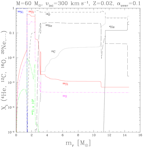
Figure 13: Variations of the abundance (in mass fraction) as a function of the lagrangian mass coordinate, $m_{r}$, at the end of central Si–burning for the rotating 60 $M_{\sun}$. Note that the ⁴⁴Ti abundance (dotted–long dashed line) is enhanced by a factor 1 000 for display purposes.

The major characteristics of the models are summarised in Tables 1 and 2. In order to calculate lifetimes of the central burning stages, we take the start of a burning stage when $0.003$ in mass fraction of the main burning fuel is burnt. We consider that a burning stage is finished when the main fuel mass fraction drops below $10^{-5}$. The results would be the same if we had chosen $10^{-4}$ or $10^{-6}$. Neon burning is an exception because neon abundance does not drop significantly before the end of oxygen burning. We therefore consider the end of Ne–burning when its abundance drops below $10^{-3}$. Therfore the lifetimes for Ne–burning are to be considered as estimates. Other authors use the duration of the convective core as the lifetime. We note that using the duration of convective cores as central burning lifetimes instead of threshold values of the central abundance of the main fuel would yield results very similar to those given in Table 1 for H, He, O and Si–burning stages. The core sizes are given at the end of central silicon–burning and at the last model calculated (which corresponds to a different evolutionary stage in the non–rotating and the rotating models as seen above). The inner limit of each core is the star centre. The outer limit is the point in mass where the sum of the mass fraction of the main burning products (helium for $M_{\alpha}$, carbon and oxygen for $M_{\rm{CO}}$, ²⁸Si–⁴⁴Ti for $M_{\rm{Si}}$ and ⁴⁸Cr–⁵⁶Ni for $M_{\rm{Fe}}$) becomes less than $0.75$ (superscript 75) or $0.50$ (superscript 50). Another possibility to define the outer limit of a core is to consider the lagrangian mass where the mass fraction of the main fuel (helium for the CO cores) drops below $10^{-2}$. The CO cores thus obtained are given in Tables 1 and 2 (superscript 01). These limits are suitable for most masses (see Fig. 15). However, for very massive stars (see Fig. 13), shell He–burning transforms most helium into carbon and oxygen and one could also consider that $M_{\rm{CO}}$ includes the whole star. In that case we suggest another definition of $M_{\rm{CO}}$, which we name $M_{\rm{CO}}^{\rm{int}}$, defined by $M_{\rm{CO}}^{\rm{int}}=M_{\rm{CO}}^{01}+\int_{M_{\rm{CO}}^{01}}^{M_{\rm{\alpha}}^{01}}X_{\rm{CO}}\ dm$, where $X_{\rm{CO}}$ is the sum of ¹²C and ¹⁶O mass fractions. This definition gives an intermediate value between $M_{\rm{CO}}^{01}$ and the total actual mass of the star.

Table 2: Same as Table 1 for the 12 $M_{\sun}$ models. The non–rotating model starts Ne–burning off–centre and the burning never reaches the centre. The unburnt Ne–O core, is given by $M_{\rm{Ne-O}}$.

Initial model properties
$M_{\rm{ZAMS}}$	12	12
$\upsilon_{\rm{ZAMS}}$	0	300
Lifetime of burning stages
$\tau_{\rm{H}}$	1.56 (7)	2.01 (7)
$\tau_{\rm{He}}$	2.08 (6)	1.58 (6)
$\tau_{\rm{C}}$	6.47 (3)	6.09 (3)
$\tau_{\rm{Ne}}$	-	1.138
$\tau_{\rm{O}}$	-	4.346
End of calculation
$M_{\rm{total}}$	11.524	10.199
$M_{\alpha}^{75}$	3.141	3.877
$M_{\rm{CO}}^{\rm{int}}$	1.803	2.258
$M_{\rm{CO}}^{01}$	1.723	2.077
$M_{\rm{Si}}^{50}$	0.805	1.340
$M_{\rm{Ne-O}}$	0.096	-

3.1 Hertzsprung–Russell (HR) diagram

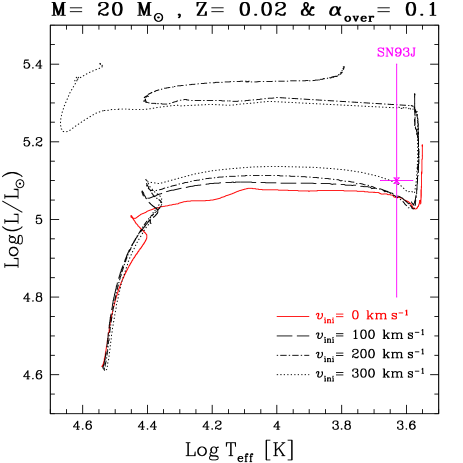
Figure 1: HR–diagram for 20 $M_{\sun}$ models: solid, dashed, dotted-dashed and dotted lines correspond respectively to $v_{\rm{ini}}$= 0, 100, 200 and 300 km s^-1. We also indicate the position of the progenitor of SN1993J.

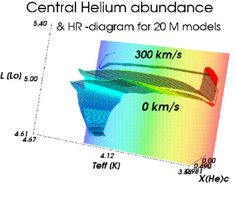
Figure 2: 3D HR diagram with central helium mass fraction as the third dimension for non–rotating and rotating 20 $M_{\sun}$ models.

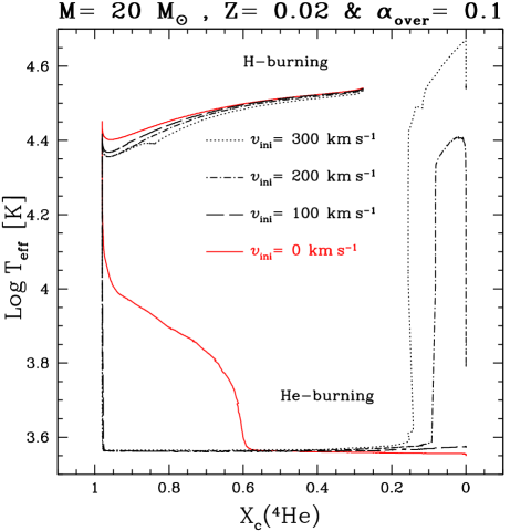
Figure 3: $T_{\rm{eff}}$ vs central helium mass fraction for 20 $M_{\sun}$ models: solid, dashed, dotted-dashed and dotted lines correspond respectively to $v_{\rm{ini}}$= 0, 100, 200 and 300 km s^-1.

The models calculated in the present work follow the same tracks as the models from Meynet & Maeder (2003). This is expected since the only difference between the two sets of models is the inclusion of dynamical shear in the present models. Here we concentrate on the 20 $M_{\sun}$ models. For that purpose, we also calculated 20 $M_{\sun}$ models with initial rotation velocities of 100 and 200 km s^-1 (Hirschi et al., 2003b). The tracks of the 20 $M_{\sun}$ models are presented in Figs. 1, 2 and 3. Figure 1 shows the evolutionary tracks of the four different 20 $M_{\odot}$ stars in the HR–diagram. The non–rotating model ends up as a red supergiant (RSG) like the model of other groups (see Heger & Langer, 2000; Limongi et al., 2000). However, the rotating models show very interesting features. Although the 100 km s^-1 model remains a RSG, the 200 km s^-1 model undergoes a blue loop to finish as a yellow–red supergiant whereas the 300 km s^-1 model ends up as a blue supergiant (BSG). Thus rotation may have a strong impact on the nature of the supernova progenitor (red, blue supergiant or even Wolf–Rayet star) and thus on some observed characteristics of the supernova explosion. For instance the shock wave travel time through the envelope is proportional to the radius of the star. Since RSG radii are about hundred times BSG ones, this travel time may differ by two orders of magnitude depending on the initial rotational velocity.

When does the star evolve back to the blue after a RSG phase and why ? Figure 2 is a 3D plot of the HR–diagram (in the plane) and the extra dimension represents the central helium mass fraction, $X_{\rm{c}}(^{4}\rm{He})$. The extra dimension allows us to follow H, He and post He–burnings within a same diagram. Indeed, $X_{\rm{c}}(^{4}\rm{He})$ increases during the main sequence, then decreases during He–burning and finally is equal to zero during the post He–burning evolution. We can see that:

• For the non–rotating model, He–burning starts when the star crosses the HR–diagram (Log $T_{\rm{eff}}\sim 4$) and the star only reaches the RSG stage halfway through He–burning. Finally, the star luminosity rises during shell He–burning.

• For the $\upsilon_{\rm{ini}}=300$ km s^-1 model, the star is more luminous and becomes a RSG before He–burning ignition. These two factors favour higher mass loss rates and the star loses most of its hydrogen envelope before He–burning is finished. Thus the star evolves towards the zone of the HR diagram where homogeneous helium stars are found, i.e. in the blue part of the HR diagram. We can see that the star track still evolves during shell He–burning.

Figure 3 is a projection of Fig. 2 in the Log $T_{\rm{eff}}$ versus $X_{\rm{c}}(^{4}\rm{He})$ plane. Although less intuitive than the 3D plot, it is more quantitative and still allows us to follow the various burning stages described above. Figure 3 shows that all the rotating models become RSG before the beginning of the He–burning phase. The 100 km s^-1 model luminosity is lower than for the 300 km s^-1 model and therefore less mass is lost during He–burning and the burning ends before the hydrogen envelope is removed. The star therefore remains a RSG. The 200 km s^-1 model evolution is similar to the 300 km s^-1 model but the extent of its blue loop is smaller. At the end of He–burning for the 200 km s^-1 model, Log $T_{\rm{eff}}=4.28$ and the star becomes redder before C–burning starts.

Although the models discussed here are for solar metallicity, one can note that the behaviours of the models with $\upsilon_{\rm{ini}}$ between 200 and 300 km s^-1 are reminiscent of the evolution of the progenitor of SN1987A. Let us recall that this supernova had a blue progenitor which evolved from a RSG stage (see e.g. the review by Arnett et al., 1989). In Fig. 1, we also indicate the position of the progenitor of SN 1993J. SN 1993J probably belongs to a binary system (Podsiaklowski et al., 1993). Nevertheless it has common points with our $\upsilon_{\rm{ini}}=$200 km s^-1 20 $M_{\sun}$ model: the star model and the progenitor of SN 1993J have approximately the same metallicity, they have a similar position in the HR–diagram taking into account the uncertainties and they both have a small hydrogen rich envelope, making possible a change from type II to type Ib some time after the explosion.

3.2 Lifetimes

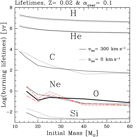
Figure 4: Burning lifetimes as a function of the initial mass and velocity. Solid and dotted lines correspond respectively to rotating and non–rotating models. Long–dashed and dotted–dashed lines are used for rotating and non–rotating Ne–burning lifetimes to point out that they are to be considered as estimates (see text).

The lifetimes are presented in Tables 1 and 2 and plotted in Fig. 4. We focus here our discussion on the effects of rotation on the lifetimes of the advanced burning phases. A discussion of the earlier stellar evolutionary phases can be found in previous papers (Meynet & Maeder, 2003; Heger et al., 2000). For C–burning onwards, we have two patterns:

$M\lesssim 30M_{\sun}$:

Since the He–burning temperature is higher in rotating stars, the $\frac{\rm{C}}{\rm{O}}$ ratio is smaller at the end of He–burning and therefore the C–burning lifetimes are shorter. If C–burning is less important, less neon is produced and neon burning is also shorter. The trends for O– and Si–burnings are similar.

$M\gtrsim 30M_{\sun}$:

The rotating stars become more rapidly WR stars and are more eroded by winds. The central temperatures for rotating models are therefore equal or even smaller than for non-rotating models. This leads to higher $\frac{\rm{C}}{\rm{O}}$ ratios, longer C– and Ne–burnings phases.

These two groups correspond to mass ranges where rotational mixing ($M\lesssim 30M_{\sun}$) or mass loss ($M\gtrsim 30M_{\sun}$) dominates the other process.

4 Rotation evolution

4.1 Dynamical shear

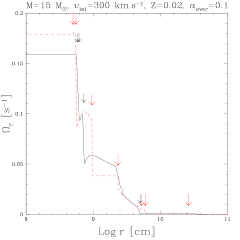
Figure 5: $\Omega$ variations as a function of the radius inside 15 $M_{\sun}$ models: the dashed line is a profile from a model without dynamical shear and the solid line from a model with dynamical shear and $Ri_{c}=1$ during core O–burning. The long and short arrows indicate the zones where $Ri<1$ in the model without and with dynamical shear respectively. Note that the profiles do not differ significantly.

As said in Sect. 2.3.1, we calculated three $\upsilon_{\rm{ini}}=300$ km s^-1 15 $M_{\sun}$ models to see the impact of dynamical shear and the importance of the value of $Ri_{c}$: one model without dynamical shear, one with $Ri_{c}=1/4$ and the last one with $Ri_{c}=1$. In Fig. 5, the variation of the angular velocity, $\Omega$, as a function of the radius is shown inside 15 $M_{\odot}$ stellar models in the core O–burning phase. Arrows indicate the zones which are unstable against dynamical shear instability. These zones remain unstable during the whole post core He–burning phase. Our simulations show that the characteristic timescale of the dynamical shear ($\propto R^{2}/D$) is always very short when using Eq. (5) for the dynamical shear diffusion coefficient. Indeed, we obtain diffusion coefficients between $10^{12}$ and $10^{14}$ cm² sec^-1. This is in general one or two orders of magnitude larger than using the expressions given by Brüggen & Hillebrandt (2001) or Heger et al. (2000). However, the extent of the unstable zones is very small, a few thousandths of $M_{\sun}$. Therefore the shear mainly smoothens the sharp $\Omega$-gradients as can be seen in Fig. 5 but does not transport angular momentum or chemical species over long distances. The general structure and the convective zones are similar between the model without dynamical shear and the one with dynamical shear.

Concerning the Richardson criterion, there is no significant difference between the models using $Ri_{c}=1/4$ and $Ri_{c}=1$. Except for the 15 $M_{\odot}$ model discussed in this subsection, all the other models were computed with $Ri_{c}=1/4$.

4.2 Angular velocity, $\Omega$, and momentum evolution

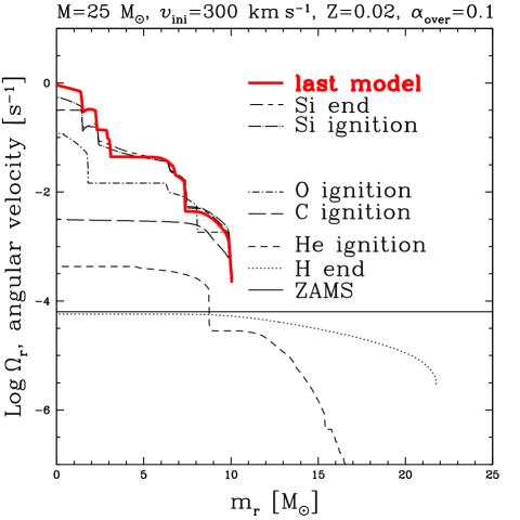
Figure 6: Angular velocity as a function of the lagrangian mass coordinate, $m_{r}$ inside the 25 $M_{\sun}$ model ($v_{\rm{ini}}$= 300 km s^-1) at various evolutionary stages.

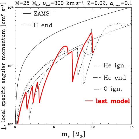
Figure 7: Local specific angular momentum profiles for the 25 $M_{\sun}$ model ($v_{\rm{ini}}$= 300 km s^-1) at different evolutionary stages.

Figure 6 shows the evolution of $\Omega$ inside the 25 $M_{\odot}$ model from the ZAMS until the end of the core Si–burning phase. The evolution of $\Omega$ results from many different processes: convection enforces solid body rotation, contraction and expansion respectively increases and decreases $\Omega$ in order to conserve angular momentum, shear (dynamical and secular) erodes $\Omega$–gradients while meridional circulation may erode or build them up and finally mass loss may remove angular momentum from the surface. If during the core H–burning phase, all these processes may be important, from the end of the MS phase onwards, the evolution of $\Omega$ is mainly determined by convection, the local conservation of the angular momentum and, for the most massive stars only during the core He–burning phase, by mass loss.

During the MS phase, $\Omega$ decreases in the whole star. When the star becomes a red supergiant (RSG), $\Omega$ at the surface decreases significantly due to the expansion of the outer layers. Note that the envelope is gradually lost by winds in the 25 $M_{\sun}$ model. In the centre, $\Omega$ significantly increases when the core contracts and then the $\Omega$ profile flattens due to convection. $\Omega$ reaches values of the order of $1\,s^{-1}$ at the end of Si–burning. It never reaches the local break–up angular velocity limit, $\Omega_{c}$, although, when local conservation holds, $\Omega_{r}/\Omega_{c}\propto r^{-1/2}$.

Figure 7 shows the evolution of the specific angular momentum, $j_{r}=2/3\,\Omega_{r}r^{2}$, in the central region of a 25 $M_{\odot}$ stellar model. The specific angular momentum remains constant under the effect of pure contraction or expansion, but varies when transport mechanisms are active. One sees that the transport processes remove angular momentum from the central regions. Most of the removal occurs during the core H–burning phase. Still some decrease occurs during the core He–burning phase, then the evolution is mostly governed by convection, which transports the angular momentum from the inner part of a convective zone to the outer part of the same convective zone. This produces the teeth seen in Fig. 7. The angular momentum of the star at the end of Si–burning is essentially the same as at the end of He–burning (by end of He–burning, we mean the time when the central helium mass fraction becomes less than $10^{-5}$). This result is very similar to the conclusions of Heger et al. (2000) on this issue. They find that the angular momentum profile does not vary substantially after C–burning ignition (see Sect. 7.5 for a comparison). It means that we can estimate the pre–supernova angular momentum by looking at its value at the end of He–burning. We calculated, for the 25 $M_{\sun}$ model, the angular momentum of its remnant (fixing the remnant mass to 3 $M_{\sun}$). We obtained ${\cal L}_{\rm rem}=2.15\,10^{50}$g cm² s^-1 at the end of He–burning and ${\cal L}_{\rm rem}=1.63\,10^{50}$g cm² s^-1 at the end of Si–burning. This corresponds to a loss of only 24%. In comparison, the angular momentum is decreased by a factor $\sim$5 between the ZAMS and the end of He–burning. This shows the importance of correctly treating the transport of angular momentum during the Main Sequence phase.

5 Internal structure evolution

5.1 Central evolution

Figure 8 (left) shows the tracks of the 15 and 60 $M_{\sun}$ models throughout their evolution in the central temperature versus central density plane (Log $T_{\rm{c}}$–Log $\rho_{\rm{c}}$ diagram). Figure 8 (right) zooms in the advanced stages of the 12, 20 and 40 $M_{\sun}$ models. It is also very instructive to look at Kippenhahn diagrams (Figs. 11 and 12) in order to follow the evolution of the structure. Figure 9 helps understand the cause of the movements in the Log $T_{\rm{c}}$–Log $\rho_{\rm{c}}$ diagram.

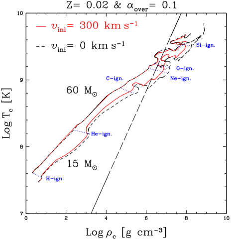
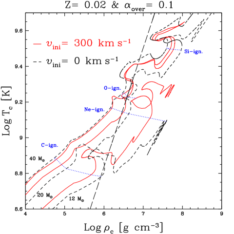
Figure 8: Log $T_{\rm{c}}$ vs Log $\rho_{\rm{c}}$ diagrams: Left: evolutionary tracks for the 15 and 60 $M_{\sun}$ models. Right: evolutionary tracks zoomed in the advanced stages for the 12, 20 and 40 $M_{\sun}$ models. Solid lines are rotating models and dashed lines are non–rotating models. The ignition points of every burning stage are connected with dotted lines. The additional long dashed line corresponds to the limit between non–degenerate and degenerate electron gas ($P^{\rm{el}}_{\rm{perfect\,gas}}=P^{\rm{el}}_{\rm{degenerate\,gas}}$).

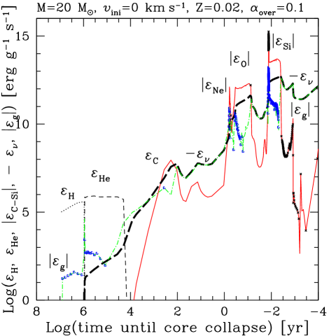
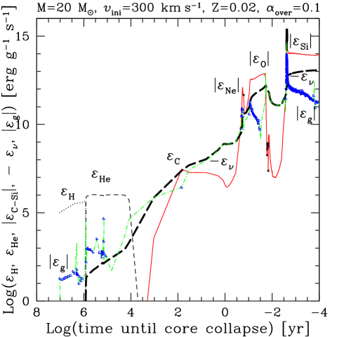
Figure 9: Log of the energy production rate per unit mass at the star center as a function of the time left until core collapse for the non–rotating (left) and rotating (right) 20 $M_{\sun}$ models. Nuclear energy production rates during H– and He–burnings are shown in dotted ($\varepsilon_{H}$) and dashed ($\varepsilon_{He}$) lines respectively. The solid line corresponds to the nuclear energy production rate in absolute value during the advanced stages ($\varepsilon_{C}$–$\varepsilon_{Si}$). Black crosses are drawn on top of the line whenever the energy production rate is negative. The thick long dashed line is the energy loss rates due to neutrinos multiplied by -1 ($-\varepsilon_{\nu}$). Finally the gravitational energy production rate in absolute value is plotted in the dotted–dashed line ($\varepsilon_{g}$). Blue squares are plotted on top when this energy is negative. Note that negative gravitational energy production corresponds to an expansion.

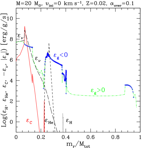
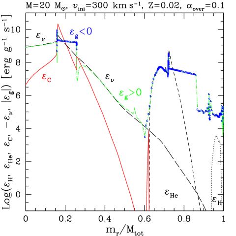
Figure 10: Log of the energy production rate per unit mass as a function of $m_{r}/M_{tot}$ during shell C–burning for the non–rotating (left) and rotating (right) 20 $M_{\sun}$ models. The solid line corresponds to the nuclear energy in absolute value during C–burning ($\varepsilon_{C}$). Nuclear energy during H– and He–burnings are shown in dashed ($\varepsilon_{He}$) and dotted ($\varepsilon_{H}$) lines respectively. The long dashed line is the energy loss rates due to neutrinos multiplied by -1 ($-\varepsilon_{\nu}$). Finally the gravitational energy production rate in absolute value is plotted in the dotted–dashed line ($\varepsilon_{g}$). Blue squares are plotted on top when this energy is negative. Note that negative gravitational energy corresponds to an expansion.

We clearly identify two categories of stellar models: those whose evolution is mainly affected by mass loss (with an inferior mass limit of about 30 $M_{\sun}$), and those whose evolution is mainly affected by rotational mixing (see also Sect. 3.2). We can see that for the 12, 15, 20 $M_{\sun}$ models, the rotating tracks have a higher temperature and lower density due to bigger cores. The bigger cores are due to the effect of mixing, which largely dominates the structural effects of the centrifugal force. On the other hand, for the 40 and 60 $M_{\sun}$ models, mass loss dominates mixing effects and the rotating model tracks in the Log $T_{\rm{c}}$–Log $\rho_{\rm{c}}$ plane are at the same level or below the non–rotating ones.

In order to understand the evolutionary tracks in the Log $T_{\rm{c}}$–Log $\rho_{\rm{c}}$ plane, we need to look at the different sources of energy at play. These are the nuclear energy, the neutrino and photon energy losses and the gravitational energy (linked to contraction and expansion). The different energy production rates at the star center are plotted in Fig. 9 as a function of the time left until core collapse. Going from the left to the right of Fig. 9, the evolution starts with H–burning where $\varepsilon_{H}$ dominates. In response, a small expansion occurs ($\varepsilon_{g}$ negative and very small movement to lower densities in the 15 $M_{\sun}$ model during H–burning in Fig. 8). At the end of H–burning, the star contracts non–adiabatically ($T\sim\rho^{1/3}$, every further contraction is also non–adiabatic). The contraction increases the central temperature. This happens very quickly and is seen in the sharp peak of $\varepsilon_{g}$ between H– and He–burnings. When the temperature is high enough, He–burning starts, $\varepsilon_{He}$ dominates and contraction is stopped. Note that during the H– and He–burning phases, most of the energy is transferred by radiation on thermal timescale. After He–burning, neutrino losses ($\varepsilon_{\nu}<0$) overtake photon losses. This accelerates the evolution because neutrinos escape freely. During burning stages, the nuclear energy production stops the contraction if $\varepsilon_{nucl}\sim-\varepsilon_{\nu}$ (see C–burning for the rotating model) or even provoke an expansion when $\varepsilon_{nucl}>-\varepsilon_{\nu}$ (most spectacular during Si–burning). Central density decreases when the central regions expand (see Fig. 8). Once the iron core is formed, there is no more nuclear energy available while neutrino losses are still present and the core collapses.
Figure 10 shows the variation of the energy production as a function of the mass fraction inside a 20 $M_{\odot}$ stellar model at a stage during the shell C–burning phase. At the different burning shells, expansion occurs due to positive nuclear energy production. In the outer part, contraction and expansion are controlled by the photon luminosity and therefore by the opacities. In the inner regions, the energy produced either by the nuclear reactions or by contraction is evacuated by the neutrinos. In the non–rotating star, partial ionisation of helium I in the outermost layers produces a peak in the opacity ($\kappa\nearrow$). This induces an expansion of the star ($\varepsilon_{g}<0$). The situation is different for the rotating model because it has lost most of its envelope and temperatures are higher than the ionisation transition zone.
Numerically, it is important to note that the largest value for energy production rates corresponds to the nuclear one. Its maximum value is therefore used in order to determine the evolutionary time steps in our code.

5.1.1 The fate of the 12 $M_{\sun}$ models

By looking at the track of the 12 $M_{\sun}$ models in Fig. 8, we can see that rotation has a noticeable effect on the post C–burning phases. Indeed, the non–rotating model starts Ne–burning off–centre and the burning never reaches the centre. The unburnt Ne–O core, $M_{\rm{Ne-O}}$ is equal to 0.096 (see Table 2). On the other hand, the rotating model starts Ne and O–burnings in the centre. This can be seen in Fig. 11 (top). The computation of the 12 $M_{\odot}$ models were stopped during the Ne/O–burning phase. To explore their further evolution, one can use the mass limits for the Ne–cores, $M_{\rm{Ne}}$, given by Nomoto (1984):

• $M_{\rm{Ne}}=1.46$ $M_{\sun}$ is the lower limit for neon ignition in the centre.

• $M_{\rm{Ne}}=1.42$ $M_{\sun}$ is the lower limit for off–centre neon ignition where the subsequent neon burning front reaches the centre.

• $M_{\rm{Ne}}=1.37$ is the lower limit for off–centre neon ignition. In the mass range between 1.37 and 1.42 $M_{\sun}$, neon burning never reaches the centre.

Our rotating 12 $M_{\sun}$ model has $M_{\rm{Ne}}\gtrsim 1.6$ well above the lower mass limit for neon ignition in the centre. In the non–rotating model the Ne–core mass is around 1.4 $M_{\sun}$ (more quantitatively carbon mass fraction decreases from 0.01 to 0.001 between 1.45 and 1.34 $M_{\sun}$). As expected from the mass limits above, in this model, neon burning, which starts off–centre, will probably reach the centre. Then (see Nomoto & Hashimoto, 1988, Sect. 3.2: fate of stars with $10\,M_{\sun}<M_{\rm{ms}}<13\,M_{\sun}$ and references therein), electron capture will help the star to collapse making the neon/oxygen burning explosive and possibly ejecting the H and He–rich layers. Note that in our models we only follow multiple–$\alpha$ elements. We did not follow the evolution of the electron mole number, $Y_{e}$, or of neutron excess, $\eta$, neither include Coulomb corrections. Let us recall that the electron mole number, $Y_{e}=\sum_{i}Z_{i}\,Y_{i}$, and the neutron excess, $\eta=\sum_{i}(N_{i}-Z_{i})Y_{i}$, are linked by the following relation: $Y_{e}=(1-\eta)/2$ ($N_{i}$, $Z_{i}$ and $Y_{i}$ are respectively the number of neutron s, protons and the number abundance of element $i$; $Y_{i}=X_{i}/A_{i}$, where $X_{i}$ and $A_{i}$ are the mass fraction and the mass number of element $i$). Therefore the electron mole number, $Y_{e}$, is always equal to 0.5. Lower values of $Y_{e}$ (due to electron captures) and the inclusion of Coulomb corrections in the equation of state have an impact in this context. Electron captures remove electrons. This decreases the electron pressure and facilitates the collapse. Coulomb corrections generally act to decrease the iron core mass by about 0.1 $M_{\sun}$ (Woosley et al., 2002, and references therein). These omissions can be the cause of the failure of our models to follow the evolution of the 12 $M_{\sun}$ models further. These two effects however do not affect significantly the evolution of more massive stars before the shell Si–burning phase.

5.2 Kippenhahn diagrams

Figures 11–12 show the Kippenhahn diagrams for the different models. The y–axis represents the mass coordinate and the x–axis the time left until core collapse. The black zones represent convective zones. Since our calculations have not reached core collapse yet, we estimate that there is $10^{-5}\,$yr between the last model and the collapse. This value has no significant influence since it is only a small additive constant. The graph is built by drawing vertical lines at each time step where the star is convective. this discrete construction shows its weakness at the right edge of each diagram and during shell He–burning where time steps are too distant from each other to cover the surface properly. The abbreviations of the various burning stages are written below the graph at the time corresponding to the central burning stages.

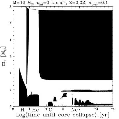
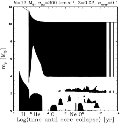
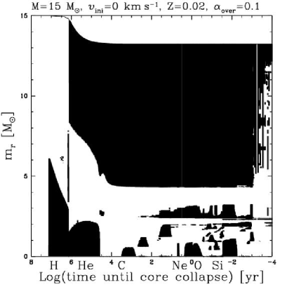
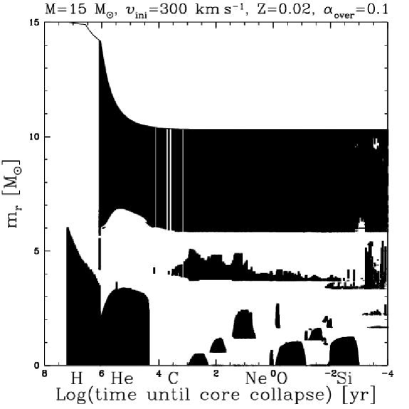
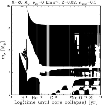
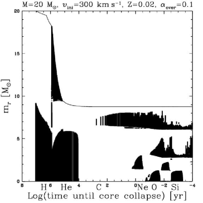
Figure 11: Kippenhahn diagrams for the non–rotating (left) and $v_{\rm{ini}}$= 300 km s^-1 (right) 12 (top), 15 (middle) and 20 (bottom) $M_{\sun}$ models. The black zones correspond to convective regions (see text).

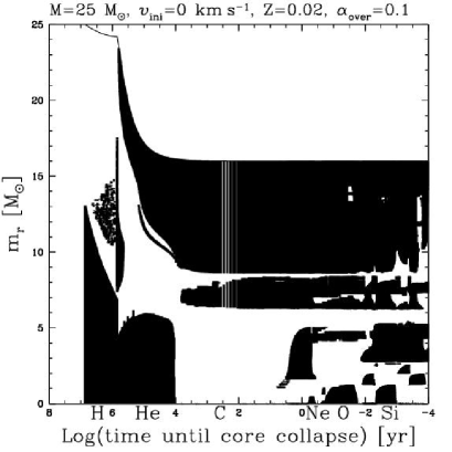
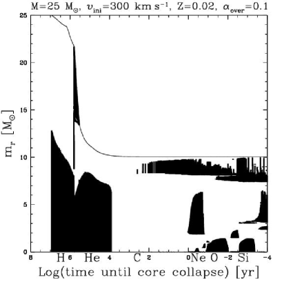
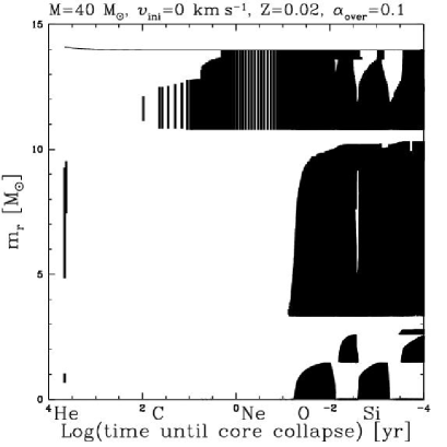
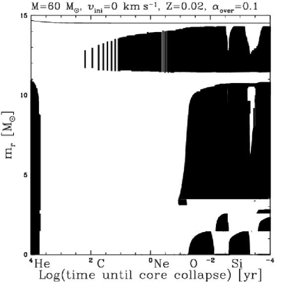
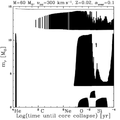
Figure 12: Kippenhahn diagram for the non–rotating (left) and $v_{\rm{ini}}$= 300 km s^-1 (right) 25 (top), 40 (middle) and 60 (bottom) $M_{\sun}$ models. The black zones correspond to convective regions (see text).

We can see the effect of the blue loops (Meynet & Maeder, 2003) in the 12 $M_{\sun}$ models on the external convective zone during the core He–burning phase. The blueward motion reduces the external convective zone or even suppresses it. We also note the complex succession of the different convective zones between central O and Si–burnings (for instance in the non–rotating 15 $M_{\sun}$ model). The difference between non–rotating and rotating models is striking in the 20 and 25 $M_{\sun}$ models. We can see that small convective zones above the central H–burning core disappear in rotating models. Also visible is the loss of the hydrogen rich envelope in the rotating models. On the other hand non–rotating and rotating 40 and 60 $M_{\sun}$ models all have very similar convective zones history after He–burning.

5.2.1 Convection during core C–burning?

Recent calculations (Heger et al., 2000) show that non–rotating stars with masses less than about 22 $M_{\sun}$ have a convective central C–burning core while heavier stars have a radiative one. Our non–rotating models agree with this. What about models of rotating stars? Figure 11 (bottom) shows the Kippenhahn diagrams for the non–rotating and rotating 20 $M_{\sun}$ models. We can see that the rotating model has a radiative core during central C–burning. It is due to the fact that the nuclear energy production rate $\varepsilon_{C}$ does not overtake $-\varepsilon_{\nu}$ (see Fig. 9 right) and therefore the central entropy does not increase enough to create a convective zone. This behaviour results from the bigger He–cores formed in rotating models. Bigger cores imply higher central temperatures during the core He–burning phase and higher central temperatures imply lower carbon content at the end of the He–burning phase. Thus less fuel is available for the core C–burning phase which does not succeed to develop a convective core. The same explanation works for more massive (rotating or non–rotating) stars. Thus the upper mass limit for a convective core during the C–burning phase is lowered by rotation, passing from about 22 $M_{\odot}$ to a value inferior to 20 $M_{\odot}$ when the initial velocity increases from 0 to 300 km s^-1.

5.3 Abundances evolution

Figures 14 and 15 show the evolution of the abundances inside the non–rotating (left) and rotating (right) 20 $M_{\sun}$ models at the end of each central burning episode. A the end of H–burning, we notice the smoother profiles in the rotating model, consequence of the rotational mixing. At the end of He–burning, we can already see the difference in core sizes and total mass. We also notice the lower C/O ratio for rotating models. At the end of O–burning, we can see that the rotating model produces much more oxygen compared to the non–rotating model (about a factor two). At the end of Si–burning, the iron and Si–cores are slightly bigger in the rotating model (see also Table 1). The yields of oxygen are therefore expected to increase significantly with rotation. This will be discussed in an forthcoming article.

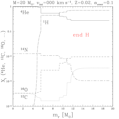
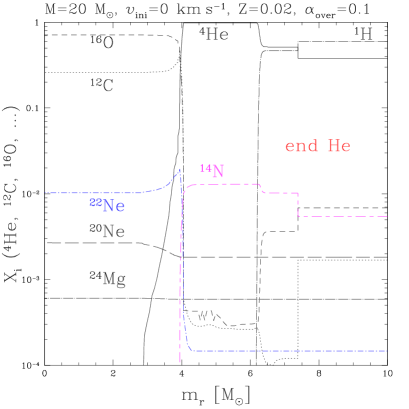
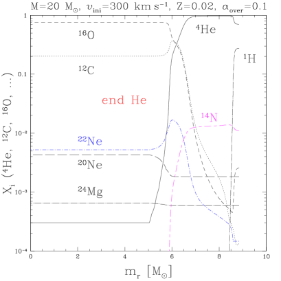
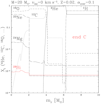
Figure 14: Variation of the abundances in mass fraction as a function of the lagrangian mass at the end of central hydrogen (top), helium (middle) and carbon (bottom) burnings for the non–rotating (left) and rotating (right) 20$M_{\sun}$ models.

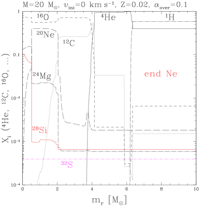
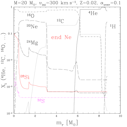
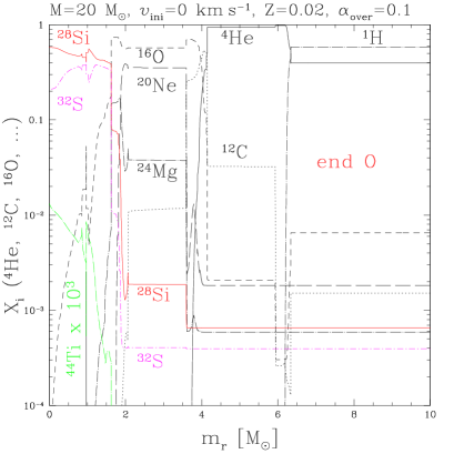
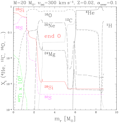
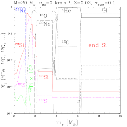
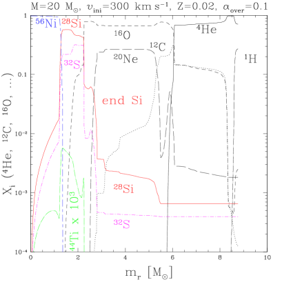
Figure 15: Variation of the abundances in mass fraction as a function of the lagrangian mass at the end of central neon (top), oxygen (middle) and silicon (bottom) burnings for the non–rotating (left) and rotating (right) 20$M_{\sun}$ models. Note that the abundance of ⁴⁴Ti (dotted–long dashed line) is enhanced by a factor 1 000 for display purposes.

6 Pre–supernova models

6.1 Core masses

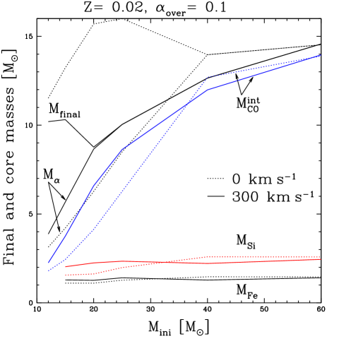
Figure 16: Core masses as a function of the initial mass and velocity at the end of core Si–burning.

Figure 16 shows the core masses (Tables 1 and 2) as a function of initial mass for non–rotating (dotted lines) and rotating (solid lines) models. Since rotation increases mass loss, the final mass, $M_{\rm{final}}$, of rotating models is always smaller than that of non–rotating ones. Note that for very massive stars ($M\gtrsim 60M_{\sun}$) mass loss during the WR phase is proportional to the actual mass of the star. This produces a convergence of the final masses (see for instance Meynet & Maeder 2004). We can also see a general difference between the effects of rotation below and above $30\,M_{\sun}$. For $M\lesssim 30\,M_{\sun}$, rotation significantly increases the core masses due to mixing. For $M\gtrsim 30\,M_{\sun}$, rotation makes the star enter at an earlier stage into the WR phase. The rotating star spends therefore a longer time in this phase characterised by heavy mass loss rates. This results in smaller cores at the pre–supernova stage. We can see on Fig. 16 that the difference between rotating and non–rotating models is the largest between 15 and 25 $M_{\sun}$.

Concerning the initial mass dependence, one can make the following remarks:

$M_{\rm{final}}$:

There is no simple relation between the final mass and the initial one. The important point is that a final mass between 10 and 15 $M_{\sun}$ can correspond to any star with an initial mass between 15 and 60 $M_{\sun}$.

$M_{\alpha}$ and $M_{\rm{CO}}$:

The core masses increase significantly with the initial mass. For very massive stars, these core masses are limited by the very important mass loss rates undergone by these stars: typically $M_{\alpha}$ is equal to the final mass for $M\gtrsim 20\,M_{\sun}$ for rotating models and for $M\gtrsim 40M_{\sun}$ for the non–rotating ones. The mass of the carbon–oxygen core is also limited by the mass loss rates for $M\gtrsim 40\,M_{\sun}$ for both rotating and non–rotating models.

$M_{\rm{Si}}$ (at the end of central Si–burning):

For rotating models, $M_{\rm{Si}}$ oscillates between 2 and 2.5 $M_{\sun}$. For non–rotating models, the mass increases regularly between 15 $M_{\sun}$ ($M_{\rm{Si}}\simeq 1.56M_{\sun}$) and 40 $M_{\sun}$ ($M_{\rm{Si}}\simeq 2.6M_{\sun}$) and stays constant for higher masses (due to mass loss).

$M_{\rm{Fe}}$ (at the end of central Si–burning):

Follows the same trend as $M_{\rm{Si}}$.

6.1.1 Final iron core masses

For non–rotating models, the masses of the iron core $M_{\rm{Fe}}$ in the last computed model (end of shell Si–burning) are very close (within 8%) to the silicon core masses, $M_{\rm{Si}}$, at the end of central Si–burning. This occurs because the extent of shell Si–burning is limited by the entropy increase produced by the second episode of shell O–burning. Therefore even though our rotating models have not reached core collapse, we can have an estimate of the final iron core mass by taking the value of $M_{\rm{Si}}$ at the end of central Si–burning. In this way, we obtain iron core masses for rotating models between 2 and 2.5 $M_{\sun}$. For non–rotating models, the mass is between 1.56 $M_{\sun}$ and 2.6 $M_{\sun}$. Rotating models have therefore more massive iron cores and we expect the lower mass limit for black hole (BH) formation to decrease with rotation.

As said in Sect. 5.1.1 about the fate of the 12 $M_{\sun}$, we did not follow the evolution of the electron mole number, $Y_{e}$, neither include Coulomb corrections. Coulomb corrections generally act to decrease the iron core mass by about 0.1 $M_{\sun}$ (Woosley et al., 2002, and references therein). Electron captures during Si–burning increases neutron excess and also reduces the electron pressure and this (with photodisintegration) will allow the core to collapse (Woosley et al., 2002). It is therefore possible that some of our models should collapse before shell Si–burning occurs. Taking this argument into account and the fact that we used Schwarzschild criterion for convection, we have to consider the value of $M_{\rm{Si}}$ at the end of core Si–burning as an upper limit for the final iron core mass.

6.2 Internal structure

As well as the chemical composition (abundance profiles and core masses) of the pre–supernova star, other parameters, like the density profile, the neutron excess (not followed in our calculations), the entropy and the total radius of the star, play an important role in the supernova explosion. Figure 17 shows the density, temperature, radius and pressure variations as a function of the lagrangian mass coordinate at the end of the core Si–burning phase. Since the rotating star has lost its envelope, this truly affects the parameters towards the surface of the star. The radius of the star (BSG) is about one percent that of the non–rotating star (RSG). As said above this modifies strongly the supernova explosion. We also see that temperature, density and pressure profiles are flatter in the interior of rotating models due to the bigger core sizes.

Figure 17: Profiles of the radius, $r$, density, $\rho$, temperature, $T$ and pressure $P$ at the end of core Si–burning for the non–rotating (left) and rotating (right) 20 $M_{\sun}$ models. The pressure has been divided by $10^{10}$ to fit it in the diagram.

7 Comparison with the literature

In this section, we compare our results (HMM hereinafter) with four other recent papers: Limongi et al. (2000) (LSC hereinafter), Woosley et al. (2002) (WHW), Rauscher et al. (2002) (RHW) and Heger et al. (2000) (HLW). Before we start the comparison, we need to mention which physical ingredients (treatment of convection, ¹²C$(\alpha,\gamma)^{16}$O reaction rate, …) they use:

• LSC use Schwarzschild criterion for convection without overshooting (except for core He–burning for which semiconvection and an induced overshooting are taken into account). For ¹²C$(\alpha,\gamma)^{16}$O, they use the rate of Caughlan et al. (1985) (CF85). Mass loss is not included.

• WHW use Ledoux criterion for convection with semiconvection. They use a relatively large diffusion coefficient for modeling semiconvection. Moreover non–convective zones immediately adjacent to convective regions are slowly mixed on the order of a radiation diffusion time scale to approximately allow for the effects of convective overshoot. For ¹²C$(\alpha,\gamma)^{16}$O, they use the rate of Caughlan & Fowler (1988) (CF88) multiplied by 1.7.

• RHW use Ledoux criterion for convection with semiconvection. They use the same method as WHW for semiconvection. For ¹²C$(\alpha,\gamma)^{16}$O, they use the rate of Buchmann (1996) (BU96) multiplied by 1.2.

• HLW use Ledoux criterion for convection with semiconvection using a small diffusion coefficient (about one percent of WHW’s coefficient) and without overshooting. For ¹²C$(\alpha,\gamma)^{16}$O, they use a rate close to Caughlan et al. (1985) (CF85). They present models with and without rotation.

• In this paper (HMM), we used Schwarzschild criterion for convection with overshooting for core H and He–burnings. For ¹²C$(\alpha,\gamma)^{16}$O, we used the rate of Angulo et al. (1999) (NACRE).

7.1 HR diagram

We remark that the present evolutionary tracks (as well as those from LSC) do not decrease in luminosity when they cross the Hertzsprung gap. This is in contrast with the tracks from HLW which present a significant decrease in luminosity when they evolve from the MS phase to the RSG phase. Models computed with the present code but using the Ledoux criterion for convection (without semiconvection) present a very similar behaviour to those of HLW. Thus the difference between the two sets of models mainly results from the different criterion used for convection.

7.2 Lifetimes

Table 3: Lifetimes of central burning stages of solar metallicity models. Lifetimes are in years with exponent in brackets (2.14 (-2)=$2.14\ 10^{-2}$).

$M_{\rm{ZAMS}}$	15 (HMM)	15 (WHW)	15 (LSC)	20 (HMM)	20 (WHW)	20 (LSC)	25 (HMM)	25 (WHW)	25 (LSC)
$\tau_{\rm{H}}$	1.13 (7)	1.11 (7)	1.07 (7)	7.95 (6)	8.13 (6)	7.48 (6)	6.55 (6)	6.70 (6)	5.93 (6)
$\tau_{\rm{He}}$	1.34 (6)	1.97 (6)	1.4 (6)	8.75 (5)	1.17 (6)	9.3 (5)	6.85 (5)	8.39 (5)	6.8 (5)
$\tau_{\rm{C}}$	3.92 (3)	2.03 (3)	2.6 (3)	9.56 (2)	9.76 (2)	1.45 (3)	3.17 (2)	5.22 (2)	9.7 (2)
$\tau_{\rm{Ne}}$	3.08	0.732	2.00	0.193	0.599	1.46	0.882	0.891	0.77
$\tau_{\rm{O}}$	2.43	2.58	2.43	0.476	1.25	0.72	0.318	0.402	0.33
$\tau_{\rm{Si}}$	2.14 (-2)	5.01 (-2)	2.14 (-2)	9.52 (-3)	3.15 (-2)	3.50 (-3)	3.34 (-3)	2.01 (-3)	3.41 (-3)

We can compare the lifetimes of the non–rotating 15, 20, 25 $M_{\sun}$ models with recent calculations presented in WHW and LSC. The comparison is shown in Table 3. As said earlier, LSC use Schwarzschild criterion with overshooting only for He–burning. WHW use Ledoux criterion with a very efficient semiconvection and allow for some overshoot. Despite important differences in the treatment of convection, all the models give very similar H–burning lifetimes which differ by less than 10 %. For the He–burning lifetimes, during which the convective core grows in mass, one can expect that the results will be significantly different depending on which convection criterion is used. This is indeed the case. Inspecting Table 3, one sees that our results are shorter by 30–50% with respect to those of WHW. In contrast when the Schwarzschild criterion is used with some overshooting as in LSC, the results are very similar (differences inferior to six percents). In the advanced stages one sees that the lifetimes obtained by the different groups are of the same order of magnitude. Let us note that the definition of the duration of the nuclear burning stages may differ between the various authors and this tends to enhance the scatter of the results. Keeping in mind this source of difference and the fact that the lifetimes vary by eight or nine orders of magnitude between the H–burning and the Si–burning phases, the agreement between the various authors appears remarkable.

7.3 Kippenhahn diagrams and convection during central C–burning

Our Kippenhahn diagrams for the non–rotating models are in good agreement with those of Rauscher et al. (2002) except that in our model the carbon and oxygen shells do not merge for the 20 $M_{\sun}$. The only noticeable difference between the structures in the advanced phase obtained in the present work and those obtained by LSC is that their 20 $M_{\sun}$ model does not have a central convective core during C–burning. This can be explained by the fact that they use the ¹²C$(\alpha,\gamma)^{16}$O rate from Caughlan et al. (1985). This rate is larger than the NACRE rate we use in our models (see Fig. 21) and therefore more ¹²C is burnt during He–burning.

7.4 Core masses

7.4.1 Non–rotating models

Table 4: Final core masses at the pre–supernova stage for different models of non–rotating stars at solar metallicity.

$M_{\rm{ZAMS}}$	15 (HMM)	15 (RHW)	15 (HLW)	15 (LSC)
$M_{\rm{total}}$	13.232	12.612	13.55	15
$M_{\alpha}^{01}$	4.168	4.163	3.82	4.10
$M_{\rm{CO}}^{01}$	2.302	2.819	1.77	2.39
$M_{\rm{Si}}^{50}$	1.842	1.808	-	-
$M_{\rm{Fe}}^{50}$	1.514	1.452	1.33	1.429
$M_{\rm{ZAMS}}$	20 (HMM)	20 (RHW)	20 (HLW)	20 (LSC)
$M_{\rm{total}}$	15.694	14.740	16.31	20
$M_{\alpha}^{01}$	6.208	6.131	5.68	5.94
$M_{\rm{CO}}^{01}$	3.840	4.508	2.31	3.44
$M_{\rm{Si}}^{50}$	2.002	1.601	-	-
$M_{\rm{Fe}}^{50}$	1.752	1.461	1.64	1.552
$M_{\rm{ZAMS}}$	25 (HMM)	25 (RHW)	25 (HLW)	25 (LSC)
$M_{\rm{total}}$	16.002	13.079	18.72	25
$M_{\alpha}^{01}$	8.434	8.317	7.86	8.01
$M_{\rm{CO}}^{01}$	5.834	6.498	3.11	4.90
$M_{\rm{Si}}^{50}$	2.577	2.121	-	-
$M_{\rm{Fe}}^{50}$	1.985	1.619	1.36	1.527

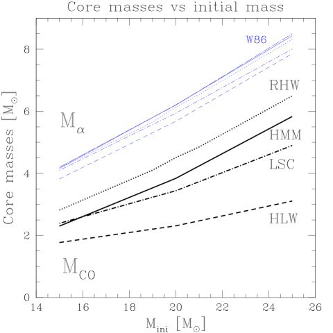
Figure 18: Variation of the He core masses, $M_{\alpha}$ (light lines), and of the CO core masses, $M_{CO}$ (heavy lines), at the pre–supernova stage in different initial mass models. Only non–rotating models are shown. The different types of line correspond to results obtained by different groups: HMM labels our results, W86 those of Woosley & Weaver (1986), RHW those of Rauscher et al. (2002), LSC those of Limongi et al. (2000) and HLW those of Heger et al. (2000).

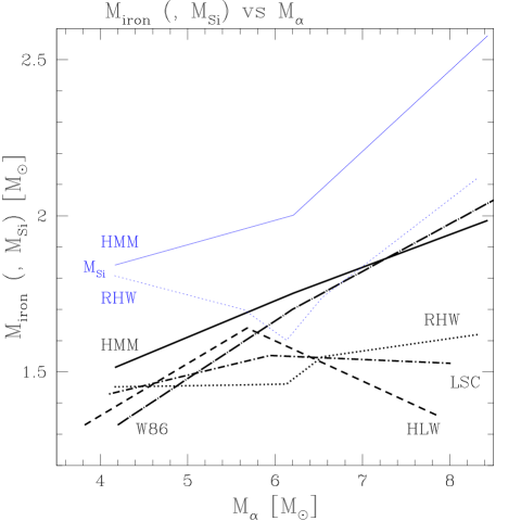
Figure 19: $M_{\rm{iron}}$ (and $M_{\rm{Si}}$) as a function of $M_{\alpha}$ for non-rotating models from different authors (see Table 4). The labels are the same as in Fig. 18. The light lines show the variation of $M_{\rm{Si}}$, the heavy lines those of $M_{\rm{iron}}$.

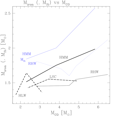
Figure 20: $M_{\rm{iron}}$ (and $M_{\rm{Si}}$) as a function of $M_{\rm{CO}}$ for non-rotating models from different authors (see Table 4). The labels are the same as in Fig. 18. The light lines show the variation of $M_{\rm{Si}}$, the heavy lines those of $M_{\rm{iron}}$.

In Table 4 the final masses and the core masses at the pre–supernova stage are given for different 15, 20 and 25 $M_{\odot}$ stellar models. The second column corresponds to the present non–rotating models, the third shows the results of Rauscher et al. (2002), the fourth those of Heger et al. (2000) and the fifth those of Limongi et al. (2000). In Fig. 18, we see that for $M_{\alpha}$, the results are very similar (within 5%) between our models and those of LSC and RHW. This can be understood by the similar outcome of the convection treatment. HLW use a small diffusion coefficient for semiconvection and logically obtain slightly smaller helium cores.

The differences between the mass of the CO cores are much greater. Let us recall here that the size of this core depends a lot on the convective criterion and also on the rate of the ¹²C($\alpha,\gamma$)¹⁶O reaction. This reaction becomes one of the main source of energy at the end of the core He–burning phase. A faster rate implies smaller central temperatures and thus increases the He–burning lifetime. This in turn will produce larger CO cores (Langer, 1991) with a smaller fraction of ¹²C. Figure 21 shows the rates used by various authors divided by the NACRE rate for the temperature range of interest.

Figure 21: Comparison of different ¹²C$(\alpha,\gamma)^{16}$O reaction rates according to various authors: CF85 labels the rate given by Caughlan et al. (1985), CF88, the rate of Caughlan & Fowler (1988), BU96 the rate of Buchmann (1996) and K02 the one of Kunz et al. (2002). All the rates are normalised to the rate given by NACRE (Angulo et al. (1999)).

Since HLW and LSC use the same rate for this reaction, most of the difference between the mass of the CO cores must have its origin in the different treatment of convection. One notes also that LSC still have slightly smaller cores than us even though they added some semiconvection and use the CF85 rate for ¹²C($\alpha,\gamma$)¹⁶O which is greater than the one adopted in our models. RHW, although they had slightly smaller $M_{\alpha}$, have larger $M_{\rm{CO}}$. This can be explained in part by the use of the rate BU96x1.2 for ¹²C($\alpha,\gamma$)¹⁶O which is larger than the NACRE rate at the end of He–burning (see Fig. 21).

In Figs 19 and 20 the Si and iron core masses obtained at the end of shell Si–burning are plotted as a function of $M_{\alpha}$ and $M_{CO}$ respectively. The present results are well in the range of values obtained by different authors for $M_{\alpha}\lesssim 6\,M_{\odot}$ ($M_{\rm ini}\lesssim 20\,M_{\odot}$). Above this mass range, our results are in agreement with those of Woosley & Weaver (1986) and significantly above the results obtained more recently by the other groups. As discussed in Sect. 6.1.1, we did not follow the evolution of the neutron excess or include Coulomb corrections. This does not affect our results until the end of core Si–burning but may affect the results plotted in Figs. 19 and 20 obtained at the end of the shell Si–burning. In this last case, the present results have to be considered as upper limits. This might be part of the explanation why our iron core masses appear to be systematically greater than those obtained in recent calculations. However one notes that Woosley et al. (2002) give a Chandrasekhar mass (lower mass limit for collapse) of 1.79 $M_{\sun}$ for the 25 $M_{\sun}$ model which is large compared to the iron core we obtain at the end of core Si–burning, implying that our 25 $M_{\sun}$ ($M_{\alpha}=8.4$ $M_{\odot}$) model may experience shell Si–burning before collapsing. Thus if we cannot discard that the final iron core masses are overestimated due to the above reason, they may also be greater than the masses obtained by other groups for other reasons. In this context it is interesting to compare the masses of the Si–burning core. The Si–cores are created by O–burning before Si–burning (except possibly a small fraction due to an additional shell O–burning during Si–burning). Their sizes are thus not dependent on the neutron excess or the Chandrasekhar mass. Looking at Fig. 19 and 20 where our Si–core masses are compared to those obtained by RHW, we see that our core masses are systematically larger. In that case the difference cannot be attributed to the neglect in our models of the electron capture reactions and of the Coulomb corrections. Our bigger cores result from the different prescription we used for convection in our models. Thus it is possible that the bigger iron cores we have obtained are due, at least in part, to the prescriptions we used for convection.

7.4.2 Rotating models

Table 5: Final core masses at the pre–supernova stage for different models of rotating stars at solar metallicity. Note that we use $M_{\rm{Si}}$ at the end of central Si–burning for the value of $M_{\rm{Fe}}$ as discussed in the text.

$M_{\rm{ZAMS}}$	15	F15B (HLW)	E15 (HLW)	20	F20B (HLW)	E20 (HLW)	25	E25 (HLW)
$M_{\rm{total}}$	10.316	12.89	10.86	8.763	14.76	11.00	10.042	5.45
$M_{\alpha}^{01}$	5.604	3.88	5.10	8.567	5.99	7.71	10.042	5.45
$M_{\rm{CO}}^{01}$	3.325	2.01	3.40	5.864	2.75	5.01	7.339	4.07
$M_{\rm{Fe}}^{50}$	2.036	1.38	1.46	2.245	1.36	1.73	2.345	1.69

We can also compare core masses of the rotating 15, 20, 25 $M_{\sun}$ models with recent calculations by Heger et al. (2000) (HLW). For $M_{\rm{Fe}}$, we use $M_{\rm{Si}}^{50}$. As discussed in section 6.1.1, this assumes that shell Si–burning occurs before the collapse and our value has to be considered as an upper limit.

The comparison is shown in Table 5. “F..B” models are the models with the same initial rotational velocity and inclusion of the $\mu$–gradients inhibiting effects on rotational mixing. These are the models which should give approximately the same results as us if uncertainties concerning the treatment of convection and particular reaction rates were small. We also show the “E..” models with a lower initial rotational velocity but without the $\mu$–gradients inhibiting effects.

One can see by comparing the results from the two models of HLW, the great dependence of the core masses on the treatment of the $\mu$–gradient inhibiting effect. The more efficient the rotational mixing (or less strong are the inhibiting effects of the $\mu$–gradients), the greater the core masses. Compared to the results obtained by HLW, one sees that our core masses are significantly greater. This essentially results from two facts: first the effects of rotation are included in our models in a different way than in the models by HLW. In particular in our models, the treatment of rotational mixing includes the inhibiting effect of $\mu$–gradients without any ad hoc parameters, and the transport of the angular momentum by the meridional circulation is properly accounted for by an advective term (Maeder & Zahn, 1998). Secondly, the present stellar models were computed with the Schwarzschild criterion with a moderate overshooting while the models of HLW were computed with the Ledoux criterion with semiconvection using a small diffusion coefficient and without overshooting.

7.5 Final angular momentum

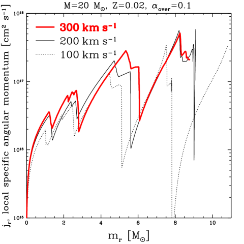
Figure 22: Comparison of the final local specific angular momentum profiles for different 20 $M_{\sun}$ models. Models with different initial velocities, $\upsilon_{\rm{ini}}$= 100, 200 and 300 km s^-1 are drawn with dotted, solid and thick solid lines respectively. We can see the convergence of the final of the final angular momentum of the core above $\upsilon_{\rm{ini}}$= 200 km s^-1.

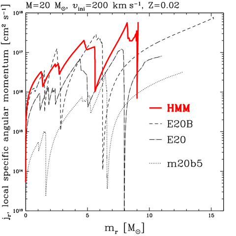
Figure 23: Comparison of the final local specific angular momentum profiles for different 20 $M_{\sun}$ models all with the same initial rotational velocity, $\upsilon_{\rm{ini}}$= 200 km s^-1. The thick solid line (HMM) corresponds to our model. The models from Heger et al. (2000) are drawn with a dashed line for model E20 (no $\mu$–barrier) and with a dotted–dashed line for model E20B ($\mu$–barrier with $f_{\mu}=0.05$). Finally, model m20b5 from Heger et al. (2003) including the effect of the magnetic fields according to Spruit (2002) is drawn with the dotted line.

Long soft gamma–ray bursts (GRBs) were recently connected with SNe (see Matheson, 2003, for example). One scenario for GRB production is the collapsar mechanism devised by Woosley (1993). In this mechanism, a star collapses into a black hole and an accretion disk due to the high angular momentum of the core. Accretion from the disk onto the central black hole produces bi–polar jets. These jets can only reach the surface of the star (and be detected) if the star loses its hydrogen rich envelope before the collapse. WR stars are therefore good candidates for collapsar progenitors since they lose their hydrogen rich envelope during the pre–SN evolution. The question to answer is whether the core of WR stars contains enough angular momentum at the pre–SN stage (the specific angular momentum, $j$, of the material just outside the core must be larger than $10^{16}\,cm^{2}\,s^{-1}$). So far only Heger and co–workers have obtained values for the angular momentum of the cores of massive stars at the pre–SN stage (Heger et al., 2000, 2003). The physical ingredients of their model have been given in Sect. 7.4.2. The comparison between our models and theirs shows that the size of the various cores depends significantly on the treatment of both convection and rotation. The evolution of angular velocity and angular momentum in the models of Heger et al. (2000, 2003), is presented in Heger et al. (2000, HLW00 hereinafter; in Figs. 8 and 9). The evolution of angular velocity and momentum in our models is described in Meynet & Maeder (2000) and in Sect. 4.2.

HLW00 show with their Fig. 9 the convergence of the final angular momentum of the core for a wide range of initial angular momentum. The dependence of the final angular momentum on the initial one for our models is displayed in Fig. 22. Models with $\upsilon_{\rm{ini}}$= 100 and 200 km s^-1 have been computed until the end of O–burning. This should not affect the comparison since the angular momentum profile does not change during Si–burning. One can see in our case that convergence only occurs above $\upsilon_{\rm{ini}}$=200 km s^-1. Indeed, the average specific angular momentum of the core (assuming a 1.7 $M_{\odot}$ core) at the end of the calculation is $1.326\,10^{16}$, $1.801\,10^{16}$ and $2.106\,10^{16}\,cm^{2}\,s^{-1}$ for $\upsilon_{\rm{ini}}$= 100, 200 and 300 km s^-1 respectively.

Concerning the evolution of the angular momentum, the general picture is the following. Mass loss removes angular momentum from the surface and transport processes (convection and rotational mixings) redistribute angular momentum inside the star (see Sect. 4.2 and the references given above for details). Here we are only concerned about the evolution of the angular momentum of the core of the star. During H–burning, both our models and models without the inhibiting effect of the $\mu$–gradient on mixing (models without “B”) from HLW00 show a large decrease of the angular momentum of the core. On the other hand, in HLW00 models including the inhibiting effect of the $\mu$–gradient (models with “B”), the core does not lose much angular momentum during H–burning. In our models, thermal turbulence is taken into account and is able to overcome the inhibiting effect of the $\mu$–gradient. HLW00 do not include the thermal effects and in their situation, the inhibiting effect of the $\mu$–gradient is almost complete even with a reduction parameter $f_{\mu}$ equal to 0.05. The different treatment of rotation (and especially the different way the inhibiting effect of the $\mu$–gradient is included) has therefore a strong impact on the evolution of the angular momentum of the core during the MS and explains the difference between the various models.

At the end of H–burning, the core contracts and the envelope expands. This restructuring phase is accompanied by a formation of a very deep external convective zone. At the same time, shell H–burning creates a short–lived intermediate convective zone. These changes may affect the angular momentum profile. The largest change in our models is the creation of a large drop of the angular momentum at the bottom of the external convective zone (see Fig. 7). This is due to the fact that convection enforces solid body rotation and therefore angular momentum is transported at the outer edge of the convective zone. No significant change is seen in the core.

During He–burning, the trend is the opposite from H–burning. In both our models and models without the inhibiting effect of the $\mu$–gradient on mixing from HLW00, the angular momentum in the core decreases slightly. On the other hand, in HLW00 models with the inhibiting effect of the $\mu$–gradient, the core loses a significant amount of angular momentum after H–burning. The reason is the following. During H–burning, in HLW00 models with the $\mu$–gradient effects on mixing, even though the core does not lose much angular momentum, the layers just above it lose angular momentum (due to various transport processes). This creates a large angular velocity gradient at the edge of the core which increases rotational mixing during He–burning. Furthermore the successive convective and semiconvective zones (due to the restructuring phase and shell H–burning) mix as well the angular momentum of the outer parts of the core with layers above the core and a large amount of angular momentum is transfered out of the core at this time. In our models (as well as those from HLW00 without $\mu$–gradient), angular momentum is transfered to the layers above the core during H–burning. This creates a smaller gradient of angular velocity at the edge of the core at the end of H–burning and thus rotational mixing is weaker during He–burning. Therefore, the angular momentum of the core does not change as much during He–burning. Note also that He–burning is ten times shorter than H–burning and that there is less time to mix. As said in Sect. 4.2, during the advanced stages, the angular momentum profile does not change substantially. Only convective zones create spikes along the profile.

The comparison of the final angular momentum profile of the different models, all with the same initial mass and surface angular velocity, is shown in Fig. 23. The thick solid line (HMM) corresponds to our model. The models from Heger et al. (2000) are drawn with a dotted–dashed line for model E20 (no $\mu$–barrier) and with a dashed line for model E20B ($\mu$–barrier with $f_{\mu}=0.05$). Finally, model m20b5 from Heger et al. (2003) including the effect of the magnetic fields according to Spruit (2002) is drawn with the dotted line. Even though the evolution of angular momentum differs between our model and model E20B (with the $\mu$–gradient effects on mixing) from Heger et al. (2000), the final value of the angular momentum of the core is very similar for these two models. This confirms the possibility of the formation of GRBs via collapsars from rotating massive stars (Woosley & Heger, 2003; Heger et al., 2003) if the effects of magnetic field (not included in our work) are small. Indeed, for example, the 25 $M_{\odot}$ model ends up as a WR star with a core having enough angular momentum ($j\gtrsim 10^{16}\,cm^{2}\,s^{-1}$ for the material just outside the core, see Fig. 7) to create a collapsar. The difference between our model and model E20 (without the $\mu$–gradient effects on mixing) from Heger et al. (2000) is probably due to the combination of the non–inclusion of the $\mu$–gradient effects on mixing and of the different treatment of meridional circulation (see Sect. 7.4.2). From model m20b5 (see Fig. 23), one sees that the inclusion of the effects of magnetic fields according to Spruit (2002) decreases significantly the final angular momentum of the core. In this situation, the core rotates too slowly and cannot produce a collapsar. We can also compare our models with the observed rotation period of young pulsars. Rotating models without the effects of magnetic fields have about 100 times more angular momentum at the pre–SN stage than the observed young pulsars (Heger et al., 2000). Models including the effects of magnetic fields according to Spruit (2002) have about 5–10 times more angular momentum at the pre–SN stage than the observed young pulsars (Heger et al., 2003). This means that in any case, additional slow down is necessary during the core collapse (Woosley & Heger, 2003; Fryer & Warren, 2004) in order to reproduce the observed rotation periods of young pulsars. The question that needs to be answered is when and how this slow down occurs. Further developments will therefore be of great importance for the formation of both NSs and GRBs. The topic of the final angular momentum of our models and its implications for further evolution will be developed in a future article.

7.6 Lower mass limit for models to reach iron core collapse

As said above, our 12 $M_{\sun}$ models have not been pursued beyond the O and Ne–burning phases for the rotating and non–rotating models respectively. Nevertheless, we think that the rotating model has the potential to reach an iron core while the non–rotating model does not. Recent calculations done by Heger et al. (2000) are similar to ours on that point: Their non–rotating models as well as the rotating models E12B, F12B and G12B neither reach core–collapse. Only the model E12 reaches core collapse but the physics used in that last model does not include $\mu$–gradient inhibiting effects on rotationally induced mixing. At the same time, recent non–rotating 13 $M_{\sun}$ models in Woosley et al. (2002) and Limongi et al. (2000) reach core–collapse. Therefore we expect the lower mass limit for non–rotating models to reach the standard iron core collapse to be around 12–13 $M_{\sun}$ in agreement with Nomoto & Hashimoto (1988). Our rotating models tend to show that this limit should be lower for rotating stars. A finer grid of models around 12 $M_{\sun}$ would help constraining this limit.

8 Conclusion

The Geneva evolution code has been improved in order to model the pre–supernova evolution of rotating massive stars. We extended the nuclear reaction network with a multiple–$\alpha$ elements chain between carbon and nickel for the advanced burning stages. We also stabilized the internal structure equations using Sugimoto’s prescription (Sugimoto, 1970). Finally, we added dynamical shear to the other rotationally induced mixing processes (secular shear and meridional circulation).

We calculated a grid of stellar models at solar metallicity with and without rotation and with masses equal to 12, 15, 20, 25, 40 and 60 $M_{\sun}$.

Concerning the evolution of rotation itself during the advanced stages, the angular velocity increases regularly with the successive contraction of the core while the angular momentum does not change significantly (only convection creates spikes along its profile). This means that we can have a good estimate of the pre–collapse angular momentum at the end of He–burning. Comparing our pre–SN models with the criteria for collapsar progenitors (Woosley & Heger, 2003), we find that WR stars are possible progenitors of collapsars. However, in this work we neglected the effects of magnetic fields. Further developments will be very interesting for the formation of both GRBs and neutron stars. Dynamical shear, although very efficient, only smoothens sharp angular velocity gradients but does not transport angular momentum over great distances.

We find that rotation significantly affects the pre–supernova models by the impact it has during H and He–burnings. We clearly see the two mass groups where either rotationally induced mixing dominates for $M<30M_{\sun}$ or rotationally increased mass loss dominates for $M>30M_{\sun}$ as already discussed in Meynet & Maeder (2003).

We show that rotation affects the lower mass limits for the presence of convection during central carbon burning, for iron core collapse supernovae and for black hole formation. The effects of rotation on pre–supernova models are most spectacular for stars between 15 and 25 $M_{\sun}$. Indeed, rotation changes the supernova type (IIb or Ib instead of II), the total size of progenitors (Blue instead of Red SuperGiant) and the core sizes by a factor $\sim 1.5$ (bigger in rotating models). For Wolf-Rayet stars ($M>30M_{\sun}$) even if the pre–supernova models are not different between rotating and non–rotating models, their previous evolution is different (Meynet & Maeder, 2003). We also compare our results with the literature. The biggest differences are the final mass and the various core masses. We obtain bigger core masses and this should have a strong impact on yields.

Future developments are planned to be able to follow the evolution until core collapse as well as follow neutron excess and detailed nucleosynthesis during the entire evolution.