COMO School of Physics

[Star Cluster Ecology] The ecology of black holes in star clusters S. F. Portegies Zwart
University of Amsterdam

1 Introduction

In this lecture we investigate the formation and evolution of black holes in star clusters.

The star clusters we investigate are generally rich, containing more than $10^{4}$ stars, and with a density exceeding $10^{4}$ stars/pc³. Among these are young populous clusters, globular cluster and the nuclei of galaxies.

Under usual circumstances black holes are formed from stars with a zero-age main-sequence (ZAMS) mass of at least 25–30 ${\rm M}_{\odot}$  (Maeder 1992; Portegies Zwart, Verbunt & Ergma 1997; Ergma & van den Heuvel 1998). These stars live less than about 10 Myr, after which a supernova results in a black hole in the range of 5–20 ${\rm M}_{\odot}$  (Fryer & Kalogera, 2001). The rest of the mass is lost from the star in the windy phase proceeding the supernova or in the explosion itself (Heger 2003). For a Scalo (1986) or Kroupa & Weidner (2003) initial mass functions (IMF), variants of Salpeter (1955), one in 2300-3500 stars collapse to a black hole. So black holes are rare, but still, the Milky-way Galaxy is populated by 30 to 40 million black holes. In the remainder we will refer to these relatively common type of black holes as stellar mass black holes or simply as BH.

Supermassive black holes (SMBH) are, with about one per galaxy, among the rarest single objects in the universe. They have masses of about $10^{6}$ to $10^{10}$ ${\rm M}_{\odot}$  which also makes them among the most massive single objects in the Universe. The best evidence for the existence of a supermassive black hole comes from the orbit of the star S2 which is in a 15.2 year orbit around an unseen object (Schödel et al.  2002). The mass of this black hole is $3.7\pm 1.5\times 10^{6}$ ${\rm M}_{\odot}$, which puts it directly at the bottom of the mass scale for SMBH’s (see also fig. 17).

The gap in mass between stellar mass black holes and supermassive black holes may be bridged by a third type, often referred to as intermediate mass black holes (IMBH).

In this chapter our main interest is the formation and evolution of these black hole families in star clusters. Also the possible evolutionary link between stellar mass black holes, via intermediate mass black holes to supermassive black holes will be addressed. We mainly focus, however, on the ecology of star clusters. The term star cluster ecology was introduced in 1992 by Douglas Heggie to illustrate the complicated interplay between stellar evolution and stellar dynamics, which by their mutual interactions has similarities with biological systems.

In the here studied ecology we mainly address the gravitational dynamics, stellar evolution, binary evolution, external influence and how these seemingly separate effects work together on the star cluster, much in the same way as in an organism.

1.1 Setting the stage

The main objects of our study are clusters of stars. There are a number of distinct families of star clusters, with one common characteristic: a star cluster is a self gravitating system of stars, all of which have about the same age. We make the distinction between various types, among which are: open cluster like Pleiads (see fig. 1), young dense cluster like R 136 in the 30 Doradus region of the large Magellanic cloud or the Arches cluster (see fig. 2), globular cluster like M15 (see fig. 3). If galactic nuclei contain a population of stars with similar ages we could include these in the definition. The nucleus of the Andromeda galaxy, depicted in Figure 4 is an example, though the stellar population in its nucleus has probably a large spread in ages.

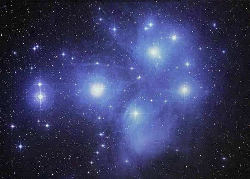
Figure 1: The Pleiads open star cluster (image by David Malin) contains a few thousand stars in a volume of a several parsec cubed.

Figure 1 shows the $\sim 115$ Myr old star cluster Pleiads, at a distance of about 135 pc (Pinfield et al.  1998; Raboud & Mermilliod 1998; Bouvier et al 1998). This cluster contains about 2000 stars, half of which are contained in a sphere with a radius of about 8 pc.

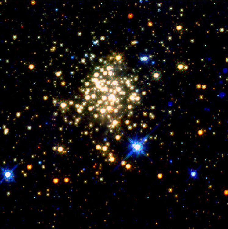
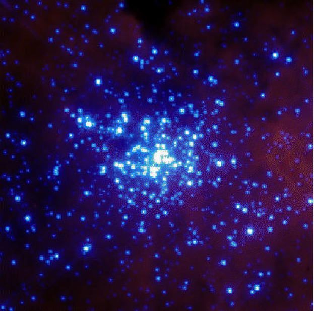
Figure 2: Left: Arches star cluster (HST image by Figer et al.  1999). At a projected distance of $\sim 30$ pc from the Galactic center this cluster is strongly influenced by external forces. The cluster on the image still looks quite symmetric since we only observe the inner part.
Right: The young dense star cluster R136 (NGC 2070, HST image by N. Walborn)in the 30 Doradus region of the large Magellanic cloud.

Figure 2 shows Hubble space telescope (HST) images of two well known young dense star clusters, Arches (to the left) and NGC 2070 (right) in the Large Magellanic Cloud. These clusters are the prototypical examples of young dense star cluster (YoDeCs), which are young ($\ {\raise-2.15277pt\hbox{$\buildrel<\over{\sim}$}}\ 10$ Myr), massive $\sim 10^{4}$ ${\rm M}_{\odot}$  and dense $n\ {\raise-2.15277pt\hbox{$\buildrel>\over{\sim}$}}\ 10^{5}$ stars/pc³. The two clusters show also that the class of young dense star clusters hosts two families of star clusters; the strongly tidally perturbed cluster (like Arches) and the isolated cluster (like R 136).

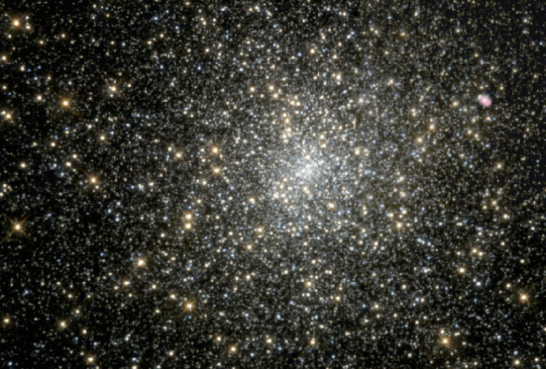
Figure 3: The globular cluster M15 (NGC 7078, HST image by Guhathakurta).

Figure 3 give a Hubble’s view of the core collapsed globular cluster M 15 (Guhathakurta 1996). It is one of the old globular star clusters in the Milky-way’s halo, contains about a million stars, and the central density is of the order of $n\ {\raise-2.15277pt\hbox{$\buildrel>\over{\sim}$}}\ 10^{5}$ stars/pc³. No core has been measured in the density profile, and therefore this cluster is identified as a collapsed globular (Harris 1996, http://physun.physics.mcmaster.ca/Globular.html).

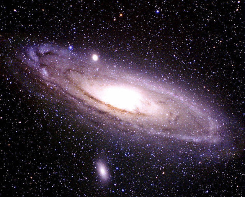
Figure 4: The Andromeda galaxy (M31, image by Jason Ware).

In figure 4 we show an image of the Andromeda Galaxy A total of 693 candidate globular clusters were found in recent 2MASS MIR observations (Galleti 2004). It is still unclear why M31 has more than trice as many globular clusters than the Milky-way Galaxy. Note also that there are no YoDeCs observed in M31, which is also somewhat puzzling, as the Milky-way Galaxy has at least four.

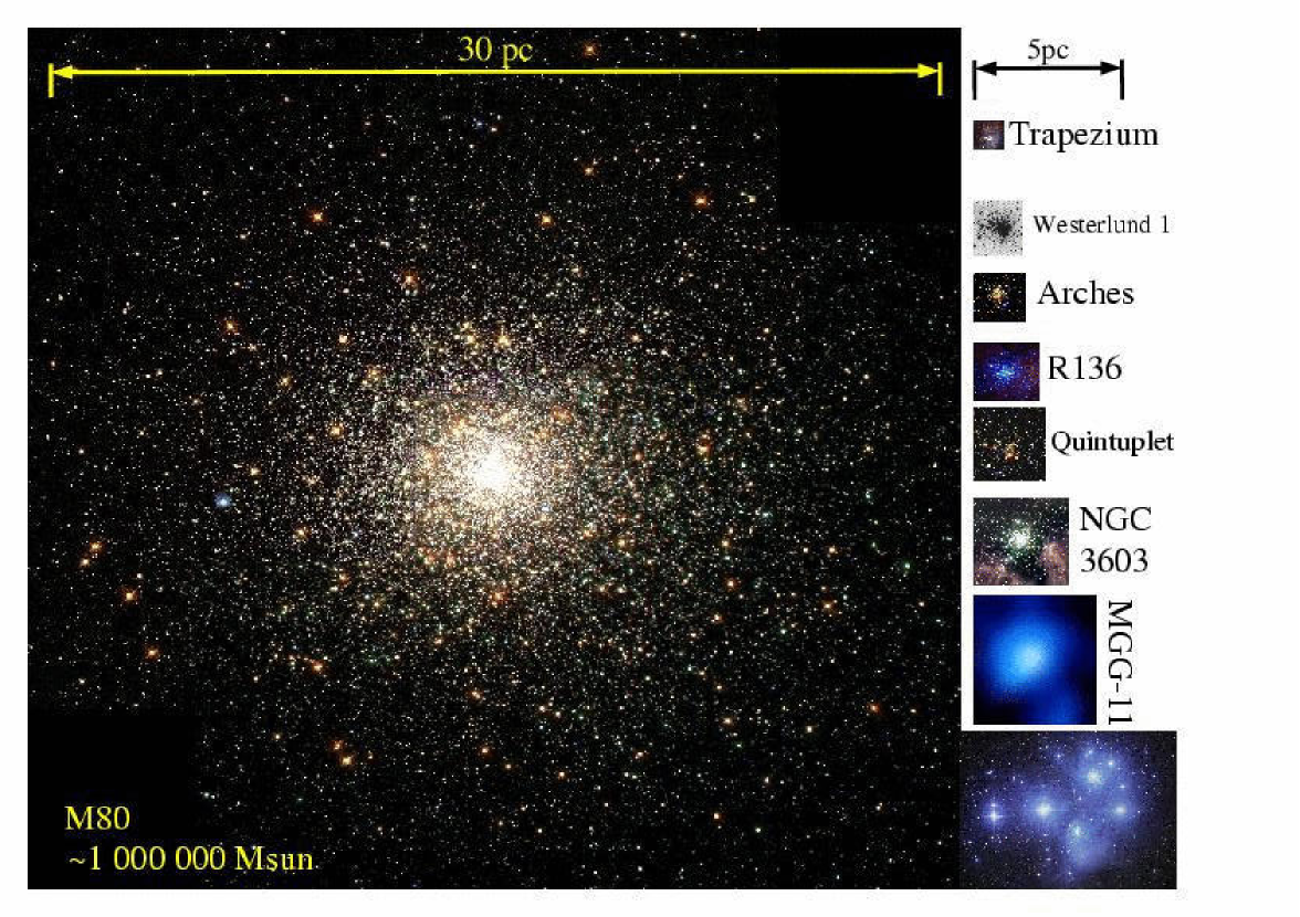
Figure 5: Star clusters in the correct physical scale. The Galaxy fig. 4 was left out for practical reasons. Images are from: M80 (F. Ferraro); Trapezium cluster (HST image by . Bally, D. Devine, R. Sutherland, and D. Johnson); Westerlund 1 (2MASS image by S. van Dyk); Arches (HST image by Figer, 1999); R 136 (HST image by N. Walborn); Quintuplet (HST image by Figer 1999); MGG-11 (VLT image by McCrady et al 2003); Pleiads (AAT image by D. Malin).

In figure 5 we place a few well known star clusters in retrospect. All cluster images are on the same scale. It is interesting to see is how large the globular cluster M80 is compared to some depicted open clusters (Pleiads) and compared to the known Galactic YoDeCs (Arches, Quintuple, NGC3603 and Westerlund 1).

Table 1: Overview of selected parameters for young dense clusters (Massey & Hunter 1998), globular clusters (Djorgovski & Meylan, 1994) and galactic nuclei (Schrödel et al. 2002). The first three columns list the cluster type, the total mass (in solar units) and the virial radius (in pc). For globulars the total mass and virial radius are given as distributions with a mean and the standard deviation around the mean. The orbital separation (in solar units) for a 1000 $kT$ binary consisting of two 10 ${\rm M}_{\odot}$  stars is given in the fourth column. The fifth and sixth columns list the expected number of black-hole binaries that are formed by the cluster and the fraction of these binaries which merge within 12 Gyr (allowing $\sim 3$ Gyr for the formation and ejection of the binaries and assuming a 15 Gyr old Universe (Freedman et al. 2001). The contributions to the total black hole merger rate per star clusters per year (MR) are given in the final column (for details see § 3.4). The bottom row contains estimated parameters for the zero-age population of globular clusters in the Galaxy.
^⋆ Estimate for the parameters at birth for the population of globular clusters.

cluster	M/${\rm M}_{\odot}$	${r_{\rm vir}}$/pc	$1000\,kT$	$N_{\rm b}$	$f_{\rm merge}$	MR
type	[$\log$]	[$\log$]	[${\rm R}_{\odot}$]			[Myr-1]
Populous	4.5	-0.4	420	7.9	7.7%	0.0061
Globular	$5.5\pm 0.5$	$0.5\pm 0.3$	315	150	51 %	0.0064
Nucleus	$\sim 7$	$\ {\raise-2.15277pt\hbox{$\buildrel<\over{\sim}$}}\ 0$	$\ {\raise-2.15277pt\hbox{$\buildrel<\over{\sim}$}}\ 3.3$	2500	100 %	0.21
Globular⋆	$6.0\pm 0.5$	$0\pm 0.3$	33	500	92 %	0.038

There appears to be a clear relation between the number of globular clusters, like M15 (see fig. 3), and the Hubble type of the host galaxy. This relation is expressed in the specific number of globular clusters $S_{\rm N}$. For open clusters and YoDeCs no such relation is known, but young star clusters are particularly abundant in starburst and interacting galaxies like the Antennae and M82.

Table 2 lists the space densities and specific numbers of globular clusters $S_{N}$ per $M_{v}=-15$ magnitude (van den Bergh 1984) for various Hubble types of galaxies. The values given for $S_{N}$ in Table  2 are corrected for internal absorption; the absorbed component is estimated from observations in the far infrared.

$$S_{N}=N_{GC}10^{0.4(M_{v}+15)}.$$ (1)

Here $N_{G}C$ is the total number of globular clusters in the galaxy under consideration. The estimated number density of globular clusters in the local Universe is

$$\phi_{GC}=8.4\,h^{3}\;{\rm Mpc^{-3}}$$ (2)

(where $h=H_{0}/100~{}{\rm km\,s}^{-1}{\rm\,Mpc}^{-1}$), slightly smaller than the result reported by Phinney (1991).

Table 2: Galaxy morphology class, space densities, average absolute magnitude (Heyl et al. 1997), and the specific frequency of globular clusters $S_{N}$ (from van den Bergh, 1995 and McLaughlin 1999). The final column gives the contribution to the total number density of globular clusters. The galaxy morphologies are identified as: E (elliptical), S0-Scd (spiral galaxies), Blue E (young blue elliptical galaxies), Sdm (blue spiral galaxies) and StarB (star burst galaxies).

Galaxy	$\phi_{\rm GN}$	$M_{v}$	$S_{N}h^{2}$	GC space density
Type	[$10^{-3}\,h_{0}$ Mpc-3]			[$h_{0}^{3}$ Mpc-3]
E–S0	3.49	-20.7	10	6.65
Sab	2.19	-20.0	7	1.53
Sbc	2.80	-19.4	1	0.16
Scd	3.01	-19.2	0.2	0.03
Blue E	1.87	-19.6	14	1.81
Sdm/StarB	0.50	-19.0	0.5	0.01

Figure 6 illustrates the concentration of clusters, expressed in the structural parameter ${\rm W}_{0}$ (King 1966), which ranges from about 1 for very shallow clusters to about 12 for very concentrated clusters. The figure shows the images of three clusters with quite different concentration ranging from $\mbox{${\rm W}_{0}$}\simeq 6$ (Omega Centauri) to $\mbox{${\rm W}_{0}$}\ {\raise-2.15277pt\hbox{$\buildrel>\over{\sim}$}}\ 12$ for the core collapsed globular cluster M15. The globular cluster 47 Tuc.  is highly concentrated, but not quite in a state of core collapse.

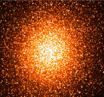
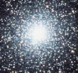
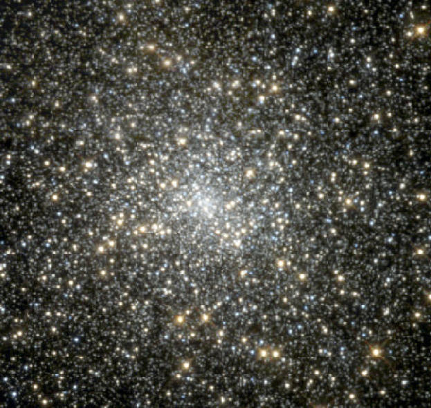
Figure 6: Three globular clusters to illustrate the effect of core collapse. Left: the rather shallow globular clusters Omega Cen.  (NGC 5139, image by P. Seitzer) with a concentration $\mbox{${\rm W}_{0}$}\simeq 6$. Middle: the concentrated cluster 47 Tuc.  (NGC 104, image by W. Keel) with concentration $\mbox{${\rm W}_{0}$}\simeq 9$. Right: the core collapsed cluster M15 (NGC 7078, HST image R. Guhathakurta) with concentration $\mbox{${\rm W}_{0}$}\simeq 12$.

1.2 Fundamental time scales

The evolution of a star cluster is dominated by two main effects; the mutual gravitational attraction between the stars and by the evolution of the individual stars. Before we discuss these two ingredients in more detail is it important do understand how they are coupled in the ecological network.

1.2.1 Stellar evolution

The fundamental timescale for stellar evolution is the nuclear burning timescale. This timescale only depends on characteristics of the stars themselves and is unrelated to any of the dynamical cluster parameters. The mass is the most fundamental parameter in the stellar evolution process; more massive stars burn-up more quickly than lower mass stars. The main sequence lifetime of a star with mass $m$ and luminosity $l$ can, to first order, be approximated with

$$t_{\rm ms}\simeq 1.1\times 10^{10}{\rm year}\left({m\over\mbox{${\rm M}_{\odot}$}}\right)\left({\mbox{${\rm L}_{\odot}$}\over l}\right).$$ (3)

After the main sequence the star generally grown to giant dimensions, but remains large only for approximately 10% of its main-sequence lifetime. Massive stars continue their evolution after central hydrogen is exhausted by burning Carbon, Neon, Oxygen and Silicon until an iron core forms, which ultimately collapse catastrophically. The result is a supernova and the formation of a compact stars. Lower mass stars cannot process all material and shed their envelope in a planetary nebula phase. This results in a white dwarf. Rather detailed stellar evolutionary tracks are published in in the form of comprehensive look-up tables (Schaller et al 1993; Meynet et al. 1994) or fitting formulae (Eggleton, Fitchet & Tout 1989; Hurley et al 2000); using a variety of stellar evolution codes.

1.2.2 Dynamical timescales

The most fundamental dynamical timescale $t_{\rm d}$ for a star cluster is the crossing time or dynamical timescale, which for a cluster with half-mass radius $R$ and dispersion velocity $\langle v\rangle$  can be written simply as

$$t_{\rm d}=R/\mbox{$\langle v\rangle$}.$$ (4)

We can generalize this by using the cluster half-mass radius and the dispersion velocity to calculate the global crossing time ${t_{\rm hm}}$  of the star cluster.

So long as stellar evolution remains relatively unimportant, the cluster’s dynamical evolution is dominated by two-body relaxation, with proceeds via the characteristic half-mass relaxation time scale (Spitzer, 1987)

$$\mbox{${t_{\rm rt}}$}=\left({R^{3}\over GM}\right)^{1/2}{N\over 8\mbox{${\ln\Lambda}$}}.$$ (5)

Here $G$ is the gravitational constant, $M$, is the total mass of the cluster, $N\equiv M/\mbox{${\langle m\rangle}$}$ is the number of stars and $r$ is the characteristic (half-mass) radius of the cluster. The Coulomb logarithm $\mbox{${\ln\Lambda}$}\simeq\ln(0.1N)={\rm O}(10)$ typically. In convenient units the two-body relaxation time becomes

$$\mbox{${t_{\rm rt}}$}\simeq 1.9\,{\rm Myr}\left({R\over 1\,{\rm pc}}\right)^{3/2}\left({M\over 1\,\mbox{${\rm M}_{\odot}$}}\right)^{1/2}\left({1\,\mbox{${\rm M}_{\odot}$}\over\mbox{$\langle m\rangle$}}\right)\left(\mbox{${\ln\Lambda}$}\right)^{-1}\,.$$ (6)

Table 3: Time scales

Time scale	symbol	bulge	globular	YoDeC	Open cluster	Como
Star	${t_{\rm ms}}$	10Gyr	10Gyr	10Myr	10Myr	100 yr
size	$R$	100pc	10pc	$\ {\raise-2.15277pt\hbox{$\buildrel<\over{\sim}$}}\ 1$pc	10pc	10 km
mass	$M$	$10^{9}$${\rm M}_{\odot}$	$10^{6}$${\rm M}_{\odot}$	$10^{5}$${\rm M}_{\odot}$	1000${\rm M}_{\odot}$	$10^{5}$pers
velocity	$\langle v\rangle$	100${\rm km~{}s}^{-1}$	10${\rm km~{}s}^{-1}$	10${\rm km~{}s}^{-1}$	1${\rm km~{}s}^{-1}$	5km/h
relaxation	${t_{\rm rt}}$	$10^{15}$yr	3 Gyr	50Myr	100Myr	10 yr
crossing	${t_{\rm hm}}$	100Myr	10 Myr	100Kyr	1Myr	1 day
collision	${t_{\rm coll}}$	10Gyr	100 Myr	10Kyr	100Myr	minutes
${t_{\rm rt}}$/${t_{\rm ms}}$		$10^{5}$	3	5	10	0.1
${t_{\rm hm}}$/${t_{\rm ms}}$		0.01	1	$10^{-4}$	0.1	0.03
${t_{\rm coll}}$/${t_{\rm ms}}$		1	0.1	$10^{-5}$	10	$10^{-7}$

Table 3 summarizes the relevant fundamental characteristics of various types of star clusters. The parameters we selected are the stellar evolution time scale, cluster mass, size and velocity dispersion. With these we can compute the relaxation time and crossing time for the various clusters. Near the bottom of the table we present the collision time: $\mbox{${t_{\rm coll}}$}\equiv 1/\Gamma_{\rm coll}$. Here $\Gamma_{\rm coll}$ is the collision rate for a cluster with stellar density $n$, and can be written as $\Gamma_{\rm coll}=n\sigma v$, where $\sigma$ is the cross section for physical collisions:

$$\sigma=\pi d^{2}\left(1+{v^{2}\over v_{\infty}^{2}}\right).$$ (7)

Here $v_{\infty}$ is the relative velocity of two stars with mass $m_{1}$ and $m_{2}$ at infinity and $v$ is the relative velocity at closest distance $d$ in a parabolic encounter, i.e: $v^{2}=2G(m_{1}+m_{2})/d$. The second term results from the gravitational attraction between the two stars, and is referred to as gravitational focusing.

We can now estimate the timescale for a collision between two stars as $\mbox{${t_{\rm coll}}$}=1/\Gamma_{\rm coll}$, which for a cluster with low velocity dispersions ($v_{\infty}\ll v$, can be written as

$$\mbox{${t_{\rm coll}}$}=7\times 10^{10}{\rm yr}\left({10^{5}{\rm pc}^{-3}\over n}\right)\left({v_{\infty}\over 10{\rm km/s}}\right)\left({\mbox{${\rm R}_{\odot}$}\over d}\right)\left({\mbox{${\rm M}_{\odot}$}\over m}\right)\ {\rm for}\ v\gg v_{\infty}.$$ (8)

For a collision between two single stars we can adopt $d\sim 3r_{\star}$ (Davies, Benz & Hills 1991).

The last column in table 3 gives, in retrospect to the star clusters, a comparison with the beautiful city in which this meeting is organized.

1.3 The effect of two-body relaxation: dynamical friction

A star cluster in orbit around the Galactic center is subject to dynamical friction, in much the same way as dynamical friction drives massive stars toward the cluster center. This causes clusters to spiral into the Galactic center and stars to the cluster center. A star cluster is generally destroyed by the tidal field when it approaches the galactic center (see Gerhard 2001). We derive here the dynamical friction time scale for a mass point in the potential of the Galactic center. The derivation of the dynamical friction time scale of a star as it spirals to the cluster center is very similar, with the major exception than the cluster potential is much more complicated that the potential of the Galaxy. We therefore opted for showing the derivation for a galaxy instead.

We assume the inpiraling object to have constant mass $M$, deferring the more realistic case of a time-dependent mass (for example in the case of a star cluster sinking to the Galactic center, see Eq.37) to McMillan & Portegies Zwart (2003).

The drag acceleration due to dynamical friction in an infinite homogeneous medium with isotropic velocity distribution that is not self-gravitating is (equation [7-18] in Binney & Tremaine, 1987)

$$a=-{4\pi\mbox{${\ln\Lambda}$}G^{2}M\rho_{G}(\mbox{${R_{\rm gc}}$})\over\mbox{$v_{\rm c}$}^{2}}\left[\mbox{${\rm erf}$}(X)-{2X\over\sqrt{\pi}}e^{-X^{2}}\right]\,.$$ (9)

Here ${\ln\Lambda}$ is the Coulomb logarithm for the Galactic central region, for which we adopt $\mbox{${\ln\Lambda}$}\sim\mbox{${R_{\rm gc}}$}/R$, ${\rm erf}$ is the error function and $X\equiv\mbox{$v_{\rm c}$}/\sqrt{2}\mbox{$v_{\rm disp}$}$, where $v_{\rm disp}$ is the one-dimensional velocity dispersion of the stars at distance ${R_{\rm gc}}$  from the Galactic center, and $v_{c}$ is the circular speed of the cluster around the Galactic center.

The mass of the Galaxy lying within the cluster’s orbit at distance ${R_{\rm gc}}$ ($\ {\raise-2.15277pt\hbox{$\buildrel<\over{\sim}$}}\ 500$ pc) from the Galactic center is (Sanders & Lowinger 1972; Mezger et al. 1996)

$$\mbox{${M_{\rm Gal}}$}(\mbox{${R_{\rm gc}}$})=4.25\times 10^{6}\left({\mbox{${R_{\rm gc}}$}\over 1\,{\rm pc}}\right)^{1.2}\;\;\mbox{${\rm M}_{\odot}$}\,.$$ (10)

Its derivative, the local Galactic density (see Portegies Zwart et al.  2001a) is

$$\rho_{G}(\mbox{${R_{\rm gc}}$})\simeq 4.06\ \times 10^{5}\left({\mbox{${R_{\rm gc}}$}\over 1\,{\rm pc}}\right)^{-1.8}\;\;\mbox{${\rm M}_{\odot}$}\,{\rm pc}^{-3}\,.$$ (11)

For inspiral through a sequence of nearly circular orbits, the function $\mbox{${\rm erf}$}(X)-{2X\over\sqrt{\pi}}\exp(-X^{2})$ appearing in Eq. 9 may be determined as follows.

Following Binney & Tremaine (p. 226), we write the equation of dynamical equilibrium for stars near the Galactic center as

$$\frac{dP}{d\mbox{${R_{\rm gc}}$}}=-\rho_{G}\frac{G\mbox{${M_{\rm Gal}}$}(\mbox{${R_{\rm gc}}$})}{\mbox{${R_{\rm gc}}$}^{2}}\,,$$ (12)

where $P=kT\rho/\mbox{${\langle m\rangle}$}$, $\frac{3}{2}kT=\frac{1}{2}\mbox{${\langle m\rangle}$}\langle v^{2}\rangle$. Since $u^{2}=\frac{1}{3}\langle v^{2}\rangle$, it follows that $P=u^{2}\rho$, and Eq. 12 becomes

$$\frac{d~{}}{dr}(u^{2}\rho)=-\frac{\rho}{r}\,\mbox{$v_{\rm c}$}^{2}\,,$$ (13)

where $v_{\rm c}$  is the circular orbital velocity at radius $R$: $\mbox{$v_{\rm disp}$}^{2}=G\mbox{${M_{\rm Gal}}$}(\mbox{${R_{\rm gc}}$})/\mbox{${R_{\rm gc}}$}$. For $\mbox{${M_{\rm Gal}}$}\propto\mbox{${R_{\rm gc}}$}^{x}$ (see Eq. 10), and assuming that $\mbox{$v_{\rm disp}$}^{2}\propto\mbox{$v_{\rm c}$}^{2}\sim\mbox{${R_{\rm gc}}$}^{x-1}$, we find $\mbox{$v_{\rm disp}$}^{2}\rho\sim\mbox{${R_{\rm gc}}$}^{2x-4}$, so

$$r\,\frac{d~{}}{dr}(\mbox{$v_{\rm disp}$}^{2}\rho)=(2x-4)\mbox{$v_{\rm disp}$}^{2}\rho=-\rho\mbox{$v_{\rm c}$}^{2}\,,$$ (14)

and hence $X=\sqrt{2-x}$. Eq. 9 then becomes

$$a=-1.2\mbox{${\ln\Lambda}$}\frac{GM}{\mbox{${R_{\rm gc}}$}^{2}}\;\left[\mbox{${\rm erf}$}(X)-{2X\over\sqrt{\pi}}\exp(-X^{2})\right]\,.$$ (15)

For $x=1.2$, $X=0.89$ and

$$a=-0.41\mbox{${\ln\Lambda}$}\frac{GM}{\mbox{${R_{\rm gc}}$}^{2}}\,.$$ (16)

Again following Binney & Tremaine, defining $L=\mbox{${R_{\rm gc}}$}\mbox{$v_{\rm c}$}$ and setting $dL/dt=a\mbox{${R_{\rm gc}}$}$, we can integrate Eq. 16 with respect to time to find an inspiral time from initial radius $R_{i}$ of

$${T_{\rm f}} \simeq \frac{1.28}{\mbox{${\ln\Lambda}$}}\frac{\mbox{${M_{\rm Gal}}$}(R_{i})}{M}\left[\frac{G\mbox{${M_{\rm Gal}}$}(R_{i})}{R_{i}^{3}}\right]^{-1/2}$$ (17)

$$\simeq 1.4\left(\frac{R_{i}}{10{\rm pc}}\right)^{2.1}\left(\frac{10^{6}\mbox{${\rm M}_{\odot}$}}{M}\right)\;{\rm Myr}$$ (18)

For definiteness, we have assumed $\mbox{${\ln\Lambda}$}\sim 4$ ($\Lambda\sim\mbox{${R_{\rm gc}}$}/R\sim 100$) in Eq. 18, corresponding to a distance of about 10–30 pc from the Galactic center.

1.4 Simulating star clusters

Stars move around due to their mutual gravity. This principle was first accurately described by Sir. Isaac Newton in 1687 in his Philosophiae naturalis principia mathematica (an excellent short biography can be found at http://www-gap.dcs.st-and.ac.uk.

Newton’s equation describe the gravitational interaction between two stars with masses $m_{1}$ and $m_{2}$ with relative positional vector ${\bf r}={\bf r}_{2}-{\bf r}_{1}$, which we can written as:

$${{\rm d}{\bf r}^{2}\over{\rm d}t^{2}}=-G{m_{1}+m_{2}\over r^{3}}{\bf r}.$$ (19)

The minus sign in the right-hand side indicates that the interaction force (${\rm d}{\bf r}^{2}/{\rm d}t^{2}$) is attractive.

This second order differential equation can be integrated in many ways. At this moment Hut and Makino are in the process of writing a series of 10 books about integrating this equation using the so called direct N-body technique. The first three volumes of this series are available at http://www.ArtCompSci.org. Other recent excellent work is published by Heggie & Hut (2003) and Aarseth (2003). Therefore instead of worrying about the intricacies of N-body  techniques we continue directly with the core problem.

First, however, it may be useful to explain a bit about the methods under consideration and some of its alternatives; it is not my intention to give a thorough overview of all the way in which you can solve an N-body  system, but it is good to have some, overview. In a direct N-body  solver you integrate the equations of motion of all stars in the system by computing the forces from each star directly. This means that the amount of work for the computer scales roughly with the square of the number of particles $N$, or in units of CPU time:

$$t_{\rm CPU}=\left(\!\!\!\!\begin{array}[]{c}N\\ 2\end{array}\!\!\!\right),$$ (20)

which for large $N$ becomes $t_{\rm CPU}=\lim_{N\rightarrow\infty}N^{2}$. This scaling becomes even worse if one imagines that the dynamical time unit in a star cluster is inversely proportional to $N$ (see Eq. 4), resulting in a time complexity which approaches $t_{\rm CPU}\propto N^{3}$. Due to this high computational cost it is at this moment not possible to integrate the equations of motion of $10^{6}$ stars for a Hubble time. The largest simulations so far have been done are $N\simeq 10^{5}$ stars for a Hubble time (Baumgardt et al 2003) and of $N=585.000$ stars for the first 12 Myr of the cluster (Portegies Zwart et al 2004).

One way to escape this conundrum is by integrating the equations of motion less accurately, or to not integrate them at all but by approximating the time evolution of the (grand)canonical ensemble of stars which forms the cluster. The (semi)approximate methods are generally harder to code and often impossible to assess, which makes fine-tuning to direct N-body  simulations inevitable. The core problem here is that a star cluster is in a delicate way not in perfect virial equilibrium. Methods which assume a vitalized state therefor have a distinct disadvantage over methods which do not explicitly require equilibrium. Often the more complex numerical coding of approximate solvers is well spend for large systems, like galaxies or cosmological simulations, in which low precision methods are preferred because of the shear number of ’stars’ which have to be modeled.

For simulating dense star clusters the best way is probably still the direct integration of the N-body  system, though competitive approaches have been taken (see e.g., § 1.4.1 and § 1.4.2).

An extensive comparison between various types of N-body codes has been performed in Heggie’s (1998) collaborative experiment, the results of which can be inspected at http://www.maths.ed.ac.uk/$\sim$douglas/experiment.html.

Recently Spinnato et al.  (2003) carry out a comprehensive comparison between three very different N-body techniques. The methods they adopt are a direct integration approach, which is, though accurate, strongly limited in the number of particles which can be integrated. For larger particle numbers they used a tree-code, and for the same system but with up to several million particles they adopted a particle-mesh technique.

1.4.1 Particle mesh

Figure 7: The different grids of SUPERBOX (Fellhauer et al.  2000) for 4 cells per dimension. The finest and intermediate grids are focused on the object of interest. Figure from Spinnato et al (2003).

To perform calculations for close-to homogeneous particle distributions a particle-mesh code is quite suitable. Grainier systems like dense star clusters are less suited, though some advances have been made by increasing resolution in substructure regions. However, caution has to be taken to make sure that the studied stellar system does not relax, as relaxation is generally not treated correctly in a particle-mesh technique. A nice example is SUPERBOX (Fellhauer et al.  2000) in which accuracy is sacrificed for speed.

In the particle-mesh technique densities are derived on Cartesian grids. Using a fast Fourier transform algorithm these densities are converted into a grid-based potential. Forces acting on the particles are calculated using these grid-based potentials, making the code nearly collision-less. To achieve high resolution at the places of interest several techniques to improve a better local accuracy are used; SUPERBOX for example, incorporates two levels of sub-grids which stay focused on the objects of interest while they are moving through the simulated area (see Fig. 7), providing higher resolution where required.

Particle mesh codes, however, will always suffer from discrete effect due to the projection of the system on a grid. The size of a grid cell however, appears to be related directly to the softening parameter $\epsilon$ used in tree codes and in some direct N-body  codes. The concept of softening as introduced by (Aarseth 1963) is a technique to prevent large angle gravitational scattering by increasing the distance between two particles with a small parameter $\epsilon$. As long as $r\gg\epsilon$ the effect of softening is not noticeable, but at close distances it has a profound effect on the behavior of the system.

In order to understand how the cell length of the particle-mesh code and the softening parameter $\epsilon$ of direct N-body  and treecodes relate with each other, we compare in Fig. 8 the results from the particle-mesh code SUPERBOX with the GADGET (Spingel et al 2001) treecode simulations for $80\,000$ particles. In this example Spinnato et al.  (2003) use a black hole of mass $0.00053$ (the mass of the inner part of the galaxy is unity in these units) to sink to the center of the Galaxy from a normalized distance. We can scale these numbers to astrophysically relevant units, in which case the black hole is $\sim 65000$ ${\rm M}_{\odot}$  and born at a distance of $\sim 8$ pc from the Galactic center. The initial orbit of the black hole was circular, but it still sinks slowly to the center of the Galaxy, due to dynamical friction (see § 1.3). Figure 8 shows the distance of the black hole to the Galactic center as a function of time for the two computer codes. The results are presented for two values of the softening parameter $\epsilon$ in the treecode and compared with two values of the cell-size in the particle mesh code.

The in-fall of the black hole, as shown in Fig. 8, depends on the values of $l$ and $\epsilon$ in a remarkably similar way; $l$ and $\epsilon$ seem to play the same qualitative role, but also quantitatively the results are quite similar.

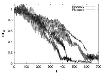
Figure 8: Spiral in of a black hole (of mass $M_{BH}\simeq 0.0005$) to the center of the Galaxy (with mass $\mbox{${M_{\rm Gal}}$}\equiv 1$). The simulations ware performed with 80,000 stars, using the same initial realization for both the treecode and the particle-mesh code. The particle-mesh simulations are run with cell size $\simeq 0.037$ (left) and $0.086$ (right); softening parameters in the treecode runs are resp. $0.030$ (left) and $0.060$ (right).

1.4.2 Tree codes

The concept of a hierarchical treecode was introduced by Apple (1985) and Barnes & Hut (1986), and is now widely used for the simulation of (near) collision-less systems. Figure 9 illustrates the concept of hierarchically deviding the spacial coordinates in the tree code. The force on a given particle in a treecode is computed by considering particle groups of ever larger size as their distance from the particle of interest increases. Force contributions from such groups are evaluated by truncated multipole expansions. The grouping is based on a hierarchical tree data structure, which is realized by inserting the particles one by one into initially empty simulation cubes. Each time two particles are in the same cube, it is split into eight ’child’ cubes, whose linear size is one half of its parent’s. This procedure is repeated until each particle is in a different cube. Hierarchically connecting such cubic cells according to their parental relation leads to the hierarchical tree data structure. The force on the particle of interest is then computed on neighboring cubes, which increase in size as they are further away. One of the interesting characteristics of tree-codes is the relatively simple parallelization by domain decomposition of the spacial coordinates (Olson & Dorband 1994); a disadvantage is the lack of support for special purpose hardware (see however Kawai et al 2004).

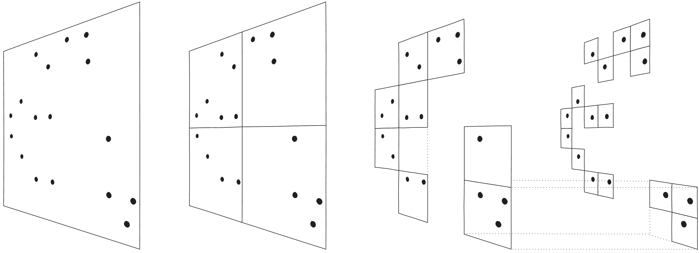
Figure 9: Schematic illustration of tree-building in a Barnes & Hut (1986) algorithm in two dimensions (from Springel, Yoshida and White, 2001). The particles are first enclosed in a single square, which is iteratively subdivided in squares of only half the size until a single particle remains per square.

In the same way we compared a particle-mesh code with a treecode in § 1.4.1, we can also compare the tree code with a direct N-body  code (see next section). In Fig. 10 such comparison is illustrated on the same simulation of the black hole which spirals to the Galactic center. Both codes are run with $N=80\,000$ and for a softening of $\epsilon\simeq 0.0037$, $0.030$ and $\epsilon\simeq 0.060$. In this comparison we adopted kira from the Starlab package as the direct N-body  code. The latter code was also run with zero softening ($\epsilon=0$) but for the treecode this did not produce reliable results.

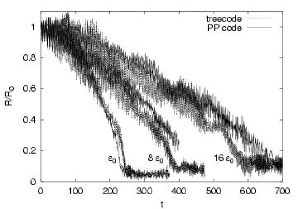
Figure 10: Comparison of results from the PP code with results from the treecode, at different values of $\epsilon$. For all cases shown here is $N=80\,000$ and $M_{BH}=0.000528$. The PP simulation with $\epsilon=8\epsilon_{0}$ has been already shown in Fig. LABEL:obs_fig. the runs ware performed with $\epsilon\simeq 0.0037$ (left), $0.030$ (middle) and $\epsilon\simeq 0.060$ (right).

Interestingly, from the comparison between the particle-mesh code, the tree code and the direct N-body  code in the figures 8 and 10 it is evident that in this practical case all three codes produce qualitatively and quantitatively the same results. One can wonder why then it is so important to perform an accurate calculation, as low resolution simulations produce results which are consistent with high precision simulations?

1.4.3 Direct N-body

The most most accurate way to simulate the dynamical evolution of a star cluster is by solving Eq. 19 using direct integration. Direct N-body  codes seem simple to write, as it is just a matter of solving Eq. 19 in small steps, but in fact a computer program that does the job accurately and quickly is very hard to write right. This technique was pioneered by von Hoerner (1960, 1963) Aarseth (1963), Aarseth & Hoyle (1964) and van Albada 1968). Excellent reviews are published in the earlier mentioned books by Hut & Heggie (2003), Aarseth (2003) and Hut & Makino (2003), but see also Aarseth & Lecar (1975). A further reference to Heggie & Mathieu (1986) cannot be omitted as this valuable paper discusses the dimension less units used in N-body  techniques, in which $M=R=G=1$.

In a direct N-body code the forces between all stars are calculated with numerical precision. The time complexity in this calculation is, as discussed earlier O($N^{3}$). In such a code, the particle motion is followed using a high-order integrator often with a predictor-corrector scheme (Makino and Aarseth 1992). These codes can generally not work with shared time steps; it saves time and gains accuracy to allow stars in a strong encounter to be updated by individual time steps. For simpler parallelization one generally adopts block time steps so that groups strongly interacting particles are integrated more frequently than weakly interacting stars (McMillan 1986a; 1986b; Makino 1991). Still special treatment for binaries and higher order hierarchies are required to prevent the code to come to a grinding halt during strong encounters.

During a time step, particle positions and velocities are first predicted to fourth order using the acceleration and “jerk” (time derivative of the acceleration), which are known from the previous step. The new acceleration and jerk are then computed, and the motion is corrected using the additional derivative information.

One of the great advantages of using a direct N-body  solver is the simplicity at which extra effects can be incorporated. Since each star in the cluster is represented by a particle in the code, individual characteristics, such as stellar properties, can be accounted for relatively easily and without loss of generality. This makes the direct N-body  method preferable for simulating star clusters where these effects are important. In our case we are interested in the evolution of black holes, which are relatively rare objects. It would therefore be best to utilize a technique in which we can also treat the black holes individually. The draw back here is that black holes are so rare that large clusters have to be simulated in order to obtain enough statistics on the black hole population.

On the other hand the gravitational N-body problem has many applications over a wide range of research fields, including informatics, computational science, geology and astronomy.

1.4.4 GRAPE family of computers

The enormous computational requirement for solving the N-body  problem with the direct method has been effectively addressed by a small team of researchers, who developed the GRAPE family of special purpose computers. GRAPE (short for GRAvity PipE) hardware was designed and built by a group of astrophysicists at the University of Tokyo (to name only the most relevant publications: Sugimoto et al. 1990; Fukushige et al 1991; Ito et al. 1991; Okumura et al 1993; Taiji et al 1996; Makino et al 1997; Kawai et al. 2000; Makino 2000; Makino et al. 2003). It may be clear that GRAPE is a very successful endeavor. The history and computational science of the GRAPE project is published by Makino & Taiji (1998).

The GRAPE family of computer are like a graphics accelerator speeding up graphics calculations on a workstation, without changing the software running on that workstation, the GRAPE acts as a Newtonian force accelerator, in the form of an attached piece of hardware. In a large-scale gravitational N-body calculation, where $N$ is the number of particles, almost all instructions of the corresponding computer program are thus performed on a standard workstation, while only the gravitational force calculations, the innermost loop, are replaced by a function call to the special-purpose hardware.

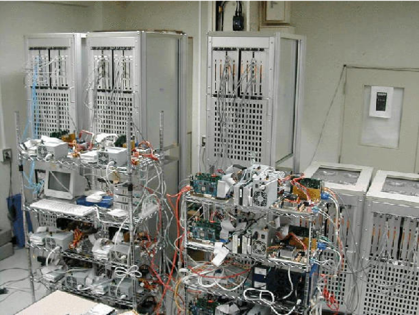
Figure 11: The large 64 Tflops GRAPE-6 configuration in Tokyo, in the summer of 2003.

Figure 11 shows the fully configured GRAPE-6 at Tokyo University.

1.5 Performing a simulations

Before starting to simulate one may want to consider what technique is most suitable. In our further discussion that will be the direct N-body  integrator. Several such computer programs are readily available. The starlab environment provides a entire library of functions and routines built around the main N-body  integrator. The package can be downloaded from http://www/manybody.org/starlab.html. But also NBODY 1–6 are available by ftp via ftp://ftp.ast.cam.ac.uk/sverre/. Both codes are large and very complicated as they have been evolving to the current sophistication over more than a decade. But simpler alternatives are available from a variety of sources (from example via: http://www.ids.ias.edu/$\sim$piet/act/comp/algorithms/starter/. A fully operational parallel N-body  code based on the above mentioned starter code can be obtained from http://carol.science.uva.nl/$\sim$spz/act/modesta/Software/index.html.

Whatever computer code you select or even if you write one from scratch, make sure that you test it. Test the code against other similar codes, test it with calculations by hand, regardless how painstaking this often is, and test it against simple problem for which the solution is known. You should develop a feeling of the regimes where the code can be trusted and in what cases extra care must be taken in interpreting the results.

Let’s assume that we have found an interesting problem, which we think we can solve with the code available. The main problem of starting a simulation then is the selection of initial conditions. Starting with wrong initial conditions is a complete waste of time. It is better to spend enough time thinking about the initial conditions, until you are convinced that they are the best choice. Possibly you want to perform several test calculations to converge to a better understanding of the question asked and the initial conditions required to give the most reliable answer.

For simulating a star cluster the primary initial conditions are:

• What are the basic cluster properties: mass, size, density profile?

• How many stars did the cluster have at birth?

• How are the stellar masses distributed?

• What is the fraction of primordial binaries?

• And what are the binary parameters: semi-major axis, eccentricity, inclination, etc.

• Do you want to include triples and higher order systems?

• and what about the shape and strength of the external tidal field of the Galaxy?

• Are there tidal shocks, spiral arms or other external potentials to worry about?

• Is there anything else to add like: passing molecular clouds or black holes, etc.

Many of the above effects have to some extend been incorporated in various calculations. And there is a rich scientific literature about the relevance and effect of many of these ingredients.

2 Theory of star cluster evolution

Now we have set the stage and discussed the tools and the techniques we can continue by discussing the global evolution of star clusters, which is characterized by three quite distinct phases; these are subsequently: A the early relaxation dominated phase, followed by phase B in which the $\sim 1$ %  (by number) most massive stars quickly evolve and lose an appreciable fraction of their mass. Finally, phase C starts when stellar evolution slows down even more and relaxation takes over until the cluster dissolves. to complete the list we can define phase D which is associated with the final dissolution of the cluster due to tidal stripping, but we will not discuss this phase in detail.

2.1 Phase A: $t\ {\raise-2.15277pt\hbox{$\buildrel<\over{\sim}$}}\ 10$Myr

In an early stage, when stellar evolution is not yet important the star cluster is dominated by its own dynamical evolution; we call this phase A. This stage in the evolution of the cluster is only relevant if $\mbox{${t_{\rm rt}}$}\ {\raise-2.15277pt\hbox{$\buildrel<\over{\sim}$}}\ 100$ Myr. For most open star clusters and for all globular clusters this stage is probably not very important, but for YoDeCs it is crucial, as we explain below.

In the following discussion we assume, for clarity, that the location in the cluster where the stars are born is unrelated to the stellar mass, i.e.: there is no primordial mass segregation. In that case, the early evolution of the star cluster is dominated by two-body relaxation, or to be more precise by dynamical friction.

In young dense clusters dynamical friction implies a characteristic time scale $t_{\rm df}$ for a massive star in a roughly circular orbit to sink from the half-mass radius $R$, to the cluster center (Spitzer 1971; 1987):

$$t_{\rm df}\simeq{\langle m\rangle\over 100\mbox{${\rm M}_{\odot}$}}{0.138N\over\ln(0.11M/100\mbox{${\rm M}_{\odot}$})}\left(R^{3}\over GM\right)^{1/2}.$$ (21)

Here $\langle m\rangle$ and $M$ are the mean stellar mass and the total mass of the cluster, respectively, $N$ is the number of stars, and $G$ is the gravitational constant. For definiteness, we have evaluated $t_{\rm df}$ for a 100 ${\rm M}_{\odot}$ star. Less massive stars undergo weaker dynamical friction, and thus must start at smaller radii in order to reach the cluster center on a similar time scale.

Dynamical friction will have two very distinct effects on the cluster: 1) it tends to produce cores in hitherto core-less clusters, and 2) it initiates core collapse in other clusters. These two statements seem to contradict each other but as we will see below, this is not the case.

2.1.1 Dynamical friction induced core development

Consider a gravitationally bound stellar system in which most of the mass is in the form of stars of mass $m\simeq\mbox{${\langle m\rangle}$}$, but which also contains a subpopulation of more massive objects with masses ${m_{\rm h}}$. The orbits of the more massive objects decay due to dynamical friction. Assume that the stellar density profile is initially a power-law in radius, $\rho(r)\propto(r/a)^{-\gamma}M/a^{3}$ with density scale length $a$ (Dehnen 1993; Merritt et al.  1994). The orbits of the massive stars decay at a rate that can be computed by equating the torque from dynamical friction with the rate of change of the orbital angular momentum. We adopt the usual approximation (Spitzer 1987) in which the frictional force is produced by stars with velocities less than the orbital velocity of the massive object. The rate at which the orbit decays, assuming a fixed and isotropic stellar background, is

$${dr\over dt}=-2{(3-\gamma)\over 4-\gamma}\sqrt{GM\over a}{\mbox{${m_{\rm h}}$}\over M}\ln\Lambda\left({r\over a}\right)^{\gamma/2-2}F(\gamma),$$ (22)

with

$$F(\gamma)={2^{\beta}\over\sqrt{2\pi}}{\Gamma(\beta)\over\Gamma(\beta-3/2)}(2-\gamma)^{-\gamma/(2-\gamma)}\int_{0}^{1}dy\ y^{1/2}\left(y+{2\over 2-\gamma}\right)^{-\beta}.$$ (23)

Here $\beta=(6-\gamma)/2(2-\gamma)$ and $\ln\Lambda$ is the Coulomb logarithm, roughly equal to 6.6 (Spinnato et al. 2003). For $\gamma=1.0$ (2.0), $F=0.19$ (0.43).

If we approximate the cluster structure with an isothermal sphere, we find (Binney & Tremaine 1987, Eq.  7-25) that a star of mass ${m_{\rm h}}$  at distance $R$ from the cluster center drifts inward at a rate given by

$$R\frac{dR}{dt}\simeq-0.43{G\mbox{${m_{\rm h}}$}\over\mbox{$\langle v\rangle$}}\mbox{${\ln\Lambda}$}.$$ (24)

Here $\langle v\rangle$  is the clusters’ velocity dispersion.

Equation 22 implies that the massive object comes to rest at the center of the stellar system in a time

$$t\approx 0.2\sqrt{a^{3}\over GM}{M\over\mbox{${m_{\rm h}}$}}\left({R_{i}\over a}\right)^{(6-\gamma)/2}$$ (25)

with $R_{i}$ the initial orbital radius.

Or, we can express the dynamical friction time in terms of the half-mass relaxation time by substituting Eq. 6 in Eq. 24 and integrate with respect to time.

$${\mbox{${t_{\rm df}}$}}\simeq 3.3{\mbox{$\langle m\rangle$}\over\mbox{${m_{\rm h}}$}}\mbox{${t_{\rm rt}}$}\,.$$ (26)

To estimate the effect on the stellar density profile, consider the evolution of an ensemble of massive particles in a stellar system with initial density profile $\rho\sim R^{-2}$. The energy released as one particle spirals in from radius $R_{i}$ to $R_{f}$ is $2\mbox{${m_{\rm h}}$}\sigma^{2}\ln(R_{i}/R_{f})$, with $\sigma$ the 1D stellar velocity dispersion. Decay will halt when the massive particles form a self-gravitating system of radius $\sim G\mbox{${M_{\rm h}}$}/\sigma^{2}$ with $\mbox{${M_{\rm h}}$}=\sum\mbox{${m_{\rm h}}$}$. Equating the energy released during in-fall with the energy of the stellar matter initially within $r_{c}$, the “core radius,” gives

$$R_{c}\approx{2G\mbox{${M_{\rm h}}$}\over\sigma^{2}}\ln\left({R_{i}\sigma^{2}\over G\mbox{${M_{\rm h}}$}}\right).$$ (27)

Most of the massive particles that deposit their energy within $R_{c}$ will come from radii $R_{i}\approx{\rm a\ few}\times R_{c}$, implying $R_{c}\approx{\rm several}\times G\mbox{${M_{\rm h}}$}/\sigma^{2}$ and a displaced stellar mass of $\sim{\rm several}\times\mbox{${M_{\rm h}}$}$ (see also Watters 2000). If $\mbox{${M_{\rm h}}$}\approx 10^{-2}M$ (Portegies Zwart & McMillan, 2000) then $R_{c}/a\approx{\rm several}\times 2\mbox{${M_{\rm h}}$}/M$ and the core radius is roughly $10\%$ of the effective radius. Merritt et al (2004) discuss this process in more detail and apply it successfully to the evolution of the core radii of large Magellanic cloud star clusters.

Evolution will continue as the massive particles form binaries and begin to engage in three-body interactions with other massive particles. These superelastic encounters will eventually lead to the ejection of most or all of the massive particles. Assume that this ejection occurs via many small ’kicks’, such that almost all of the binding energy so released can find its way into the stellar system as the particle sinks back into the core after each ejection. The energy released by a single binary in shrinking to a separation such that its orbital velocity equals the escape velocity from the core is $\sim\mbox{${m_{\rm h}}$}\sigma^{2}\ln(4\mbox{${M_{\rm h}}$}/M)$ (see also § 3.4). If all of the massive particles find themselves in such binaries before their final ejection and if most of their energy is deposited near the center of the stellar system, the additional core mass will be

$$M_{c}\approx\mbox{${M_{\rm h}}$}\ln\left({M\over\mbox{${M_{\rm h}}$}}\right)$$ (28)

e.g. $\sim 5\mbox{${M_{\rm h}}$}$ for $\mbox{${M_{\rm h}}$}/M=0.01$, similar to the mass displaced by the initial in-fall. The additional mass displacement takes place over a much longer time scale however and additional processes (e.g. core collapse) may compete with it.

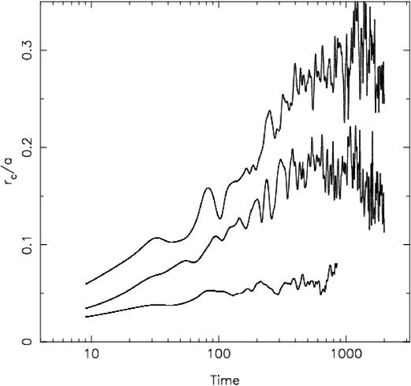
Figure 12: Evolution of the core radius, defined as the radius at which the projected density falls to one-half of its central value. Each curve is the average of the various runs at the specified value of $\gamma$, $\gamma=1$ for the top curve, 1.5 for the middle curve and $\gamma=2$ for the bottom curve (see § 2.1.1). The figure is taken from Merritt et al.  2004).

2.1.2 Dynamical friction induced core collapse

The dynamical evolution of the star cluster drives it toward core collapse (Antonov 1962; Spitzer & Hart, 1971a; 1971b) in which the central density runs away to a formally infinite value in a finite time. In an isolated cluster in which all stars have the same mass, core collapse occurs in a time $\mbox{${t_{\rm cc}}$}\simeq 15\,\mbox{${t_{\rm rt}}$}$ (Cohn 1980; Makino 1996; Joshi et al 2001).

If the dynamical friction time scale of a star cluster is shorter than the lifetime of the most massive stars, the cluster may experience an early phase of core collapse before the first supernova occurs. This can only happen if the initial half-mass relaxation time of the cluster is small $\mbox{${t_{\rm rt}}$}\ {\raise-2.15277pt\hbox{$\buildrel<\over{\sim}$}}\ 100$ Myr otherwise the most massive stars burn-up before they reach the cluster center (Portegies Zwart et al 1999; Gürkan et al 2004). The early core collapse in a cluster with small relaxation time is illustrated in figure 13, where we plot the core radius as a function of time for a number of young star clusters with a relaxation time of about 100 Myr.

The details of what exactly happens in the cluster core, and whether the cluster will experience gravothermal oscillations probably depends quite critically on the initial density profile, as we will discuss in more detail in Sect. 3.3.

When after core collapse the most massive stars explode the core radius remains highly variable, but small on average. What exactly happens at this stage is still ill understood. Naively one would expect the collapsed core to expand, as stellar mass loss drives an adiabatic expansion of the cluster. This can be been seen in the post core collapse evolution of the bottom solid curve in figure 13. Stage B starts when dynamical friction and relaxation cannot further drive the core collapse of the cluster, but expansion by stellar mass loss starts to dominate. Typically this happens around $\sim 10$ Myr.

The cluster simulated for Fig. 13 was MGG11, in the starburst galaxy M82. It contained 131072 single stars from a Salpeter initial mass function between 1 ${\rm M}_{\odot}$  and 100 ${\rm M}_{\odot}$  distributed in a King (1966) model density profile with dimension less dept $\mbox{${\rm W}_{0}$}=3$ (shallow) to $\mbox{${\rm W}_{0}$}=12$ (very concentrated). The half mass radius of these simulated clusters was 1.2 pc.

We discuss each curve in figure 13 in turn, starting at the top. The core radius of the shallow model, $c\simeq 0.67$ ($W_{0}=3$), hardly changes with time. The intermediate model $c\simeq 1.8$ ($W_{0}=8$) almost experiences core collapse near $t=3$ Myr but as stellar mass loss starts to drive the expansion of the core it never really experiences collapse. This is the moment where phase B sets in. Core collapse occurs in the $c\simeq 2.1$ ($W_{0}=9$) model near $t=0.8$ Myr. The $c\simeq 2.7$ ($W_{0}=12$) simulation is so concentrated that it starts virtually in core collapse, and the entire cluster evolution is dominated by a post-collapse phase. At this point it is not a-priory clear why core radius for models $W_{0}=9$ and $W_{0}=12$ fluctuate so much more violently than in the models with smaller concentration.

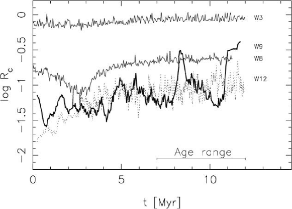
Figure 13: Evolution of the core radius for four simulations of the star cluster MGG-11. These calculations are performed with Starlab with $c\simeq 0.67$ ($W_{0}=3$), $c\simeq 1.8$ ($W_{0}=8$), $c\simeq 2.1$ ($W_{0}=9$, bold curve) and $c\simeq 2.7$ ($W_{0}=12$, dotted curve) indicated along the right edge of the figure as $W3$, $W8$, $W9$, and $W12$ respectively. The W9 curve is plotted with a heavy line to distinguish it from the curves for W8 and W12. The age range of the observed clusters MGG11 is indicated near the bottom of the figure. In figure 21 we present the evolution of the average core density for the simulations with $\mbox{${\rm W}_{0}$}=3$, 8 and 9.

2.2 Phase B: $10{\rm Myr}\ {\raise-2.15277pt\hbox{$\buildrel>\over{\sim}$}}\ t\ {\raise-2.15277pt\hbox{$\buildrel<\over{\sim}$}}\ 100$Myr

After the first few million years and until the most massive stars have turned into compact remnants, the cluster will be dominated by stellar mass loss. Since the most massive stars evolve first and sink most quickly to the cluster center, mass is lost from deep inside the potential well. A collapsed cluster may recover from its earlier core collapse due to stellar mass loss (see § 2.1.2). The dotted curve in fig. 13 (for the simulations with $\mbox{${\rm W}_{0}$}=12$) illustrates the growth of the core as a result of heating by dynamical friction and stellar evolution mass loss is quite clearly visible; it is hard to separate the two effects as both are taken into account in the calculation self consistently. For the slightly shallower initial density profile ($\mbox{${\rm W}_{0}$}=9$) the steady growth of the core radius after collapse is less clear, but the rate is similar as for $\mbox{${\rm W}_{0}$}=12$. This indicates that it is indeed mainly stellar mass loss which drives the expansion. At this stage we do not know why the core radius in the $\mbox{${\rm W}_{0}$}=9$ models fluctuate more wildly than in the $\mbox{${\rm W}_{0}$}=12$ simulations. Details probably depend quite sensitively on the presence of an intermediate mass black hole, which could form in the proceeding phase A. Such massive compact object can effectively heat the cluster core as it forms tight multiple systems with other (massive) stars (Baumgardt et al 2003).

Few studies has been carried out for clusters with short relaxation time to understand this particular evolutionary stage. For a long relaxation time $\mbox{${t_{\rm rt}}$}\ {\raise-2.15277pt\hbox{$\buildrel>\over{\sim}$}}\ 100$ Myr, it is quite clear that the cluster expands substantially during the first Gyr of its lifetime (Chernoff & Weinberg 1990; Fukushige & Heggie 1995; Takahashi & Portegies Zwart 2000; Baumgardt & Makino 2003).

The evolution of the cluster mass if given in Fig. 14 (taken from Takahashi & Portegies Zwart 2000) for a variety of particle numbers, ranging from 1024 to 32768. The first few 100 Myr of all clusters is very similar,but at later time large differences appear. In the first epoch, during the first few hundred million years, about 20% of the cluster mass is lost. This mass loss is the result of stellar evolution and, in less extend by tidal stripping. Tidal stripping and relaxation become important at later time.

Figure 14: Mass as a function of time for a number of Fokker-Planck models. The four solid lines represent the results of model Aa with 32k, 16k, 4k and 1k particles from left to right, respectively. Dotted curves present model Ie for the same numbers of particles as for model Aa (model names refer to Takahashi & Portegies Zwart, 2000). The difference between the models Ie and Aa hides in the way escaping stars are identified.

2.3 Phase C: $t\ {\raise-2.15277pt\hbox{$\buildrel>\over{\sim}$}}\ 100$Myr

After the most massive stars have turned into remnants, stellar evolution slows down, and relaxation processes can take over again. In fig. 14 this phase starts at an age of about a Gyr. The reason that stellar mass loss slows down is two-fold, 1) low mass stars remain on the main sequence longer than high mass stars, and 2) once the star turns into a remnant, the mass lost in the process is relatively small; imagine a 12 ${\rm M}_{\odot}$  star loses about 10.6 ${\rm M}_{\odot}$  by stellar wind and in the supernova explosion, whereas a 2 ${\rm M}_{\odot}$  turns into a 0.64 ${\rm M}_{\odot}$  white dwarf, losing only 1.36 ${\rm M}_{\odot}$  in the process.

The effects of mass lost from the evolving stars and mass lost from the dynamical evolution of the cluster are coupled. If stellar mass loss slows down, the cluster responses to this by a slower expansion, which again makes it less prone to tidal stripping. While the importance of stellar evolution diminishes, relaxation gradually takes over until it becomes the dominant mechanism which drives the evolution of the cluster.

The later stage of the low $N$ (1k and 2k) clusters in Fig. 14 are much stronger affected by relaxation than the high $N$ (16k and 32k) clusters. This effect was named the ski-jump problem in Portegies Zwart et al.  (1998). The transition between ski-clusters (low $N$ in fig. 14) and jump-clusters (high $N$) is a result of the non-linear interaction between the external tidal field of the parent galaxy and relaxation.

At later time during phase C dynamical friction once again become important. This time not driven by massive stars, as these have all gone supernova by now, but by the compact remnants formed in supernovae; black holes and neutron stars, but also heavy white dwarfs, blue stragglers and giants. All these stellar species are generally more massive than the mean mass, and therefore subject to dynamical friction. A similar process as in phase A starts again and the cluster may experience core collapse for the second time. It may therefore be possible that a cluster experiences two very distinct phases of core collapse, one during phase A, and again at a later time, during phase C (see also Deiters & Spurzem 2000, 2001).

In a realistic cluster, however, there are a number of additional complications which are particularly important at this stage, in part because it may take rather long to reach a state of core collapse again because the stellar mass function is rather flat now, with a relatively small difference between the least and the most massive stars. The consequence is that external influences, like disc shocks, passing molecular clouds and the presence of an external tidal field, may become particularly important at this stage, simply because they have a lot of time to accumulate their effect.

The slow-down of stellar evolution has a second important consequence, which is the termination of active binary evolution. Only relatively low mass stars are able to evolve off the main sequence, and no supernova will occur after $\sim 10^{8}$ years. It becomes therefore almost impossible to ionize hard binaries, which may effectively arrest the collapse of the cluster core (Fregeau et al.  2003). The binaries may therefore once more become dynamically important, and heat the cluster by interacting with single stars or other binaries (Heggie 1975).

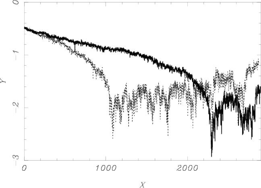
Figure 15: Evolution of the core radius for two star clusters well beyond the moment of core collapse. Time (in N-body  units) is along the x-axis and radius ($\log r$, also in N-body) units along the y-axis. Initially each cluster contained 10,000 single stars distributed in a Plummer sphere with the same realization of positions and velocities. The solid curve was computed with equal masses for all stars, the dashed curve is computed with 20% of the stars being twice as massive. these calculations ware performed without stellar evolution and the units along the axis are in dimension less N-body  units.

We illustrate phase C in Fig. 15 with a simulation of 10,000 identical point masses initially distributed in a Plummer sphere. Fig. 15 shows the evolution of the core radius of this model. Core collapse occurs at $\mbox{${t_{\rm cc}}$}\simeq 15.2\pm 0.1\,\mbox{${t_{\rm rt}}$}$ (for these initial conditions $\mbox{${t_{\rm rt}}$}\simeq 150$ N-body  time units). This result is consistent with earlier calculations of e.g., Cohn (1980) and Makino (1996). Doubling the mass of 20% of the stars reduces the core collapse time to $\mbox{${t_{\rm cc}}$}\simeq 7.2\,\mbox{${t_{\rm rt}}$}$. Making 20% of the stars 10 or 100 times more massive reduced the time of core collapse further, to $\mbox{${t_{\rm cc}}$}\simeq 1.4\,\mbox{${t_{\rm rt}}$}$ and $\mbox{${t_{\rm cc}}$}\simeq 0.16\,\mbox{${t_{\rm rt}}$}$, respectively. Clearly, the more massive stars drive the core collapse of the cluster by dynamical friction, as ${\mbox{${t_{\rm df}}$}}\simeq{\langle m\rangle\over m}\mbox{${t_{\rm rt}}$}$ (see Eq. 21, and also Watters et al.  2000).

The presence of a population of relatively massive stars, such as black holes will therefore shorten the timescale for core collapse in phase C of the cluster evolution, but even in the absence of black holes or other heavy remnants core collapse cannot be prevented. In phase A this role was played by the most massive main-sequence stars.

Note that if it is the population of dark remnants, black holes, neutron star and white dwarfs, which experience the core collapse, the lighter stars will not necessarily follow. So, the cluster may physically be in a state of core collapse, where the optical observer would measure a King profile (see Baumgardt et al 2003a; 2003b)

2.4 The consistent picture

In this section we have seen that a star cluster experiences three very distinct evolutionary phases, each of which is dominated either by relaxation or by stellar mass loss.

Figure. 16 summarized these phases in a single simulation which contains all relevant physics. The simulation presented here is carried out to illustrate the formation mechanism for intermediate mass black holes in dense young star clusters. It was performed with 131072 stars from a Salpeter initial mass function, 10% (13107) of the stars form a hard binary system with a close companion. The initial conditions for this simulation are explained in more detail in § 3.3. Here we only use the result of the simulation to illustrate the three distinct evolutionary phases in star cluster evolution, as with the adopted parameters each phase is clearly present.

The three phases, A, B and C, are identified with the horizontal bars in fig. 16. It it not a-priori clear when one phase stops and the next starts, and some gray area has to be allowed in which both, stellar evolution and relaxation, may temporarily have similar effect on the cluster. These runs ware continued till 100 Myr. Since this simulation was performed in isolation, the dissolution of the cluster will take quite a while (Baumgardt, Hut & Heggie 2002)

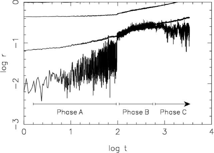
Figure 16: Evolution of the core radius (lower line) 10% and the 25% Lagrangian radii for a 128k star cluster (axis are in N-body  units). The various stages of cluster evolution are indicated near the bottom of the figure. In the early evolution of the cluster expansion of the core is driven by mass segregation, followed by phase B in which the cluster expands by stellar evolution. Near the end of the simulation the cluster tends to experience core collapse (Phase C).

3 Black holes in star clusters

In the previous sections we have set the stage for the evolution of star clusters, and we have introduced the fundamental physics. We will now continue with the evolution of black holes and their progenitors in star clusters.

3.1 The formation of intermediate mass black holes in phase A clusters

Young star clusters, with a half mass relaxation time $\mbox{${t_{\rm rt}}$}\ {\raise-2.15277pt\hbox{$\buildrel<\over{\sim}$}}\ 100$ Myr are, as we discussed in Sect. 2.1, prone to dynamical friction, and therefore are likely to experience core collapse before stellar mass loss drives the expansion of the cluster. Realistic clusters have a broad range in initial stellar masses, generally from $m_{\rm min}\ {\raise-2.15277pt\hbox{$\buildrel<\over{\sim}$}}\ 0.1$ ${\rm M}_{\odot}$  to $m_{\rm max}\ {\raise-2.15277pt\hbox{$\buildrel>\over{\sim}$}}\ 100$ ${\rm M}_{\odot}$. Adopting such a mass function as a condition at birth, the mean mass ${\langle m\rangle}$ ranges then from $\mbox{${\langle m\rangle}$}\sim 0.39$ ${\rm M}_{\odot}$  (Salpeter 1955) to about 0.65 ${\rm M}_{\odot}$  (Scalo 1986), depending on the specific mass function adopted. Here I like to stress that there is a large variety of initial mass function available, apart from the two above mentioned there are the Miller & Scalo (1979) , Koupa, Tout & Gilmore (1990) with some adjustments for high mass stars Kroupa & Weidner (2003, see also Kroupa, 2001). These mass functions seem to differ quite substantially, but for the dynamical evolution of the cluster they do not make a big difference, as for this process it is the ratio of most massive star to the mean mass which counts (see Eq. 21).

In a multi-mass system, core collapse is driven by the accumulation of the most massive stars in the cluster center. This process takes place on a dynamical friction time scale (Eq. 21). Empirically, we find, for initial mass functions of interest here, that core collapse (actually, the appearance of the first persistent dynamically formed binary systems) occurs at about (Portegies Zwart & McMillan 2000; Fregeau et al 2002)

$$\mbox{${t_{\rm cc}}$}\simeq 0.2\,\mbox{${t_{\rm rt}}$}\,.$$ (29)

This core collapse time is taken in the limit where stellar evolution is unimportant, i.e. where stellar mass loss is negligible and the most massive stars survive until they reach the cluster center, i.e.: what we called phase A in § 2.1.

Experimentally we find that starting with a Scalo (1986) initial mass function and a King (1966) $\mbox{${\rm W}_{0}$}=6$ density distribution the time to reach the first core collapse is $\mbox{${t_{\rm cc}}$}\simeq 0.19\pm 0.08\,\mbox{${t_{\rm rt}}$}$. Some of our simulations ware performed with high $W_{0}\ {\raise-2.15277pt\hbox{$\buildrel>\over{\sim}$}}\ 9$ concentration. Core collapse in these models occurred within about million years, which for these simulations corresponded to $\mbox{${t_{\rm cc}}$}\simeq 0.01\,\mbox{${t_{\rm rt}}$}$, or about 7.5% of the core relaxation time. These findings are consistent with the Monte-Carlo simulations performed by Joshi, Nave & Rasio (2001).

The collapse of the cluster core may initiate physical collisions between stars. The product of the first collision is likely to be among the most massive stars in the system, and to be in the core. This star is therefore likely to experience subsequent collisions, resulting in a collision runaway (see Portegies Zwart et al.  1999). The maximum mass that can be grown in a dense star cluster if all collisions involve the same star is ${M_{\rm run}}$, where

$${d\mbox{${M_{\rm run}}$}\over dt}=\mbox{${\cal N}_{\rm coll}$}\mbox{${\delta m_{\rm coll}}$}.$$ (30)

Here ${\cal N}_{\rm coll}$  and ${\delta m_{\rm coll}}$  are the average collision rate and the average mass increase per collision (assumed independent). We now discuss these quantities in more detail. Interestingly enough, Gürkan et al. (2004) performed comparable calculations with a Monte-Carlo N-body  code, which produces qualitatively the same results. Also the calculations of Portegies Zwart et al (2004) who used two independently developed N-body  codes (NBODY4 and Starlab), obtain similar results.

3.1.1 The collision rate ${\cal N}_{\rm coll}$

A key result from the simulations of Portegies Zwart et al. (1999) was the fact that collisions between stars generally occur in dynamically formed (“three-body”) binaries. The collision rate is therefore closely related to the binary formation rate, which we can estimate from first principles.

The flux of energy through the half-mass radius of a cluster during one half-mass relaxation time is on the order of 10% of the cluster potential energy, largely independent of the total number of stars or the details of the cluster’s internal structure (Goodman 1987). For a system without primordial binaries this flux is produced by heating due to dynamically formed binaries (Makino & Hut 1990). It is released partly in the form of scattering products which remain bound to the system, and partly in the form of potential energy removed from the system by escapers recoiling out of the cluster (Hut & Inagaki 1985). Makino & Hut argue, for an equal-mass system, that a binary generates an amount of energy on the order of $10^{2}kT$ via binary–single-star scattering (where the total kinetic energy of the stellar system is $\frac{3}{2}NkT$). This quantity originates from the minimum binding energy of a binary that can eject itself following a strong encounter. Assuming that the large-scale energy flux in the cluster is ultimately powered by binary heating in the core. It follows that the required formation rate of binaries via three-body encounters is

$$\mbox{$\Gamma_{\rm bf}$}\simeq 10^{-3}\frac{N}{\mbox{${t_{\rm rt}}$}}.$$ (31)

For systems containing significant numbers of primordial binaries, which segregate to the cluster core, equivalent energetic arguments (Goodman & Hut 1989) lead to a similar scaling for the net rate at which binary encounters occur in the core.

The above arguments apply to star clusters comprising identical point-masses. In a cluster with a range of stellar masses, three-body binaries generally form from stars which are more massive than average. After repeated exchange interactions, the binary will consist of two of the most massive stars in the cluster. Conservation of linear momentum during encounters with lower mass stars means that the binary receives a smaller recoil velocity, making it less likely to be ejected from the cluster. The binary must therefore be considerably harder—$\ {\raise-2.15277pt\hbox{$\buildrel>\over{\sim}$}}\ 10^{3}kT$—before it is ejected following a encounter with another star (see Portegies Zwart & McMillan 2000).

However, taking the finite sizes of real stars into account, it is quite likely that such a hard binary experiences a collision rather than being ejected. A strong encounter between a single star and a hard binary generally results in a resonant interaction. Three stars remain in resonance until at least one of them escapes, or a collision reduces the three-body system to a stable binary. For harder binaries it becomes increasingly likely that a collision occurs instead of ejection (McMillan 1986; Gualandris et al. 2004; Fregeau et al. 2004). In the calculations of Portegies Zwart et al. (1999) most binaries experience a collision at a binding energy of order $10^{2}kT$, considerably smaller than the binding energy required for ejection. Accordingly, we retain the above estimate of the binary formation rate (Eq. 31) and conclude that the collision rate per half-mass relaxation time is

$$\mbox{${\cal N}_{\rm coll}$}\sim 10^{-3}f_{\rm c}{N\over\mbox{${t_{\rm rt}}$}}.$$ (32)

Here we introduce $f_{\rm c}\leq 1$, the effective fraction of dynamically formed binaries that produce a collision. Note again that Eq. 32 is valid only in the limit where stellar evolution is unimportant.

The most massive star in the cluster is typically a member of the interacting binary and therefore dominates the collision rate. Subsequent collisions cause the runaway to grow in mass, making it progressively less likely to escape from the cluster. The star which experiences the first collision is therefore likely to participate in subsequent collisions. The majority of collisions thus involve one particular object—the runaway merger—generally selected by its high initial mass and proximity to the cluster center.

For systems containing many primordial binaries the above argument must be modified. Since dynamically formed binaries tend to be fairly soft—a few $kT$— the fraction of interactions with primordial binaries leading to collision is comparable to the value $f_{\rm c}$ above. However, a critical difference is that, in systems containing many binaries, the collisions involve many different pairs of stars, not just the binary containing the massive runaway. The total collision rate is therefore much higher, but most collisions do not contribute to the growth of the runaway merger. The presence of primordial binaries have little influence on the collision runaway.

3.1.2 Average mass increase per collision

Once begun, the collision runaway dominates the collision cross section. The average mass increase per collision depends on the characteristics of the mass function in the cluster core. A lower limit for stars which participate in collisions can be derived from the degree of segregation in the cluster. Inverting Eq. 21 results in an estimate (still assuming an isothermal sphere) of the minimum mass of a star that can reach the cluster core in time $t$ due to dynamical friction:

$$\mbox{${m_{\rm df}}$}=1.9\mbox{${\rm M}_{\odot}$}\,\left({1\,{\rm Myr}\over t}\right)\left({R\over 1\,{\rm pc}}\right)^{3/2}\left({m\over 1\,\mbox{${\rm M}_{\odot}$}}\right)^{1/2}\left(\mbox{${\ln\Lambda}$}\right)^{-1}\,.$$ (33)

Thus, at time $t$ and for a given mass $m$, there is a maximum radius $R$ inside of which stars of mass $m$ will have segregated to the core. The stars contributing to the growth of the runaway are likely to be among those more massive than ${m_{\rm df}}$, because their number density in the core is enhanced by mass segregation, their collision cross sections are larger, and they contribute more to ${\delta m_{\rm coll}}$ when they do collide.

The shape of the central mass function of a segregated cluster is not trivial to derive. In thermal equilibrium, the central number densities of stars of different masses would be expected to scale as

$$n_{0}(m)\sim m^{3/2}\,\frac{dN}{dm}\,,$$ (34)

where $dN/dm$ is the global initial mass function, which scales roughly as $m^{-2.7}$ at the high-mass end ($m\ {\raise-2.15277pt\hbox{$\buildrel>\over{\sim}$}}\ 10\mbox{${\rm M}_{\odot}$}$). The distribution of secondary masses (i.e. the masses of the lighter stars participating in collisions) does not follow the above simple relation. Rather, we find that stars in the core do not reach thermal equilibrium (a result generally consistent with earlier findings by Chernoff and Weinberg 1990 and Joshi, Nave & Rasio 2001), and that the dynamical nature of the collisional processes involved means that more massive stars tend to be consumed before lower-mass stars arrive in the core. In addition, most collisions involve three-body binaries and interactions with higher order multiples in a multi-mass environment.

Empirically, we find that the secondary mass distribution is quite well fit by a power-law, $dN/dm\propto m^{-2.3}$ (coincidentally very close to a Salpeter distribution). Integrating this expression from a minimum mass of ${m_{\rm df}}$ (and ignoring the upper limit) results in a mean mass increase per collision of

$$\mbox{${\delta m_{\rm coll}}$}\simeq 4\mbox{${m_{\rm df}}$}\,.$$ (35)

If we neglect stars with masses less than ${m_{\rm df}}$ and substitute Eq. 5 into Eq. 33 and Eq. 35 then the mass increase per collision can be written as

$$\mbox{${\delta m_{\rm coll}}$}\simeq 4{\mbox{${t_{\rm rt}}$}\over t}\mbox{$\langle m\rangle$}\mbox{${\ln\Lambda}$}\,.$$ (36)

This quantity remains rather constant over the entire collisional lifetime, e.g., about 3 Myr (see also § 3.3.2).

3.1.3 Lifetime of a cluster in a static tidal field

With simple expressions for ${\cal N}_{\rm coll}$ and ${\delta m_{\rm coll}}$ now in hand, we return to the determination of the runaway growth rate (Eq. 30). The evaporation of a star cluster which fills its Jacobi surface in an external potential is driven by tidal stripping. Portegies Zwart et al (2001a) have studied the evolution of young compact star clusters within $\sim 200$ pc of the Galactic center. Their calculations employed direct N-body integration, including the effects of both stellar and binary evolution and the (static) external influence of the Galaxy, and made extensive use of the GRAPE-4. They found that the mass of a typical model cluster decreased almost linearly with time:

$$M=M_{\rm 0}\left(1-\frac{t}{\mbox{${t_{\rm disr}}$}}\right)\,.$$ (37)

Here $M_{\rm 0}$ is the mass of the cluster at birth and ${t_{\rm disr}}$  is the cluster’s disruption time. Portegies Zwart et al. (2001a) found that their model clusters dissolved within about 30% of the two-body relaxation time at the tidal radius (defined by substituting the tidal radius instead of the virial radius in Eq. 5). In terms of the half-mass relaxation time, this translates to $\mbox{${t_{\rm disr}}$}=1.6$–5.4 ${t_{\rm rt}}$, depending on the initial density profile (the range corresponds to King [1966] dimensionless depths $\mbox{${\rm W}_{0}$}=3$–7; more centrally condensed clusters live longer).

Substituting Eqs. 32 and 36 into Eq. 30, and defining $M_{\rm 0}=N\mbox{${\langle m\rangle}$}$ to rewrite Eq. 37 in terms of the number of stars in the cluster, we find

$${d\mbox{${M_{\rm run}}$}\over dt} = 4\times 10^{-3}f_{\rm c}{N\mbox{${\langle m\rangle}$}\mbox{${\ln\Lambda}$}\over t}$$ (38)

$$= 4\times 10^{-3}f_{\rm c}M_{\rm 0}\mbox{${\ln\Lambda}$}\left(\frac{1}{t}-\frac{1}{\mbox{${t_{\rm disr}}$}}\right)\,.$$

Integrating from $t=\mbox{${t_{\rm cc}}$}$ to $t=\mbox{${t_{\rm disr}}$}$ results in

$$\mbox{${M_{\rm run}}$}=\mbox{${m_{\rm seed}}$}+4\times 10^{-3}f_{\rm c}M_{\rm 0}\mbox{${\ln\Lambda}$}\left[\ln\left({\mbox{${t_{\rm disr}}$}\over\mbox{${t_{\rm cc}}$}}\right)+{\mbox{${t_{\rm cc}}$}\over\mbox{${t_{\rm disr}}$}}-1\right]\,.$$ (39)

Here ${m_{\rm seed}}$ is the seed mass of the star which initiates the runaway growth, most likely one of the most massive stars initially in the cluster. With $\mbox{${t_{\rm cc}}$}\simeq 0.2\mbox{${t_{\rm rt}}$}$, Eq 39 reduces to

$$\mbox{${M_{\rm run}}$}=\mbox{${m_{\rm seed}}$}+4\times 10^{-3}f_{\rm c}M_{\rm 0}\kappa\mbox{${\ln\Lambda}$}\,,$$ (40)

where $\kappa\simeq\ln(\mbox{${t_{\rm disr}}$}/\mbox{${t_{\rm cc}}$})+\mbox{${t_{\rm cc}}$}/\mbox{${t_{\rm disr}}$}-1\sim 1$.

In figure 17 we present this relation in the form of a solid curve. We comment further on the left side of this figure where we extrapolate the relation in Eq. 40 to galactic nuclei masses.

Figure 17: The mass after a period of runaway growth as a function of the mass of the star cluster. The solid line is $\mbox{${M_{\rm run}}$}=30+8\times 10^{-4}M_{\rm 0}\mbox{${\ln\Lambda}$}$ (see Eq. 40 with $f_{\rm c}=0.2$, $\gamma=1$ and $\mbox{${\ln\Lambda}$}=\ln M_{\rm 0}/\mbox{${\rm M}_{\odot}$}$, where $M_{\rm 0}$ is the initial mass of the cluster or $10^{6}$ ${\rm M}_{\odot}$, whatever is smaller). This relation may remain valid for larger systems built up from many clusters having masses $\ {\raise-2.15277pt\hbox{$\buildrel<\over{\sim}$}}\ 10^{6}\mbox{${\rm M}_{\odot}$}$. For clusters with $M_{\rm 0}\ {\raise-2.15277pt\hbox{$\buildrel>\over{\sim}$}}\ 10^{7}$ ${\rm M}_{\odot}$  we therefore extend the relation as a dashed line. The logarithmic factor, however, remains constant, as it refers to the clusters out of which the bulge formed, not the bulge itself (Ebisuzaki et al 2001). The bottom dashed line shows $0.01\mbox{${M_{\rm run}}$}$. The five error bars to the left give a summary of the results presented by Portegies Zwart & McMillan (2002), the two right most error bars are taken from Portegies Zwart et al (2004). The error bar indicating MGG11 gives the result of estimates for the mass of the intermediate mass black hole in the M82 star cluster MGG11 (Matsumoto & Tsuru 1999; McCrady et al 2003). The Milky Way is represented by the asterisk using the bulge mass from Dwek (et al. 1995) and the black hole mass from Eckart & Genzel (1997) and Ghez (2000). Bullets and triangles (upper right) represent the bulge masses and measured black hole mass of Seyfert galaxies and Quasars, respectively (both from Wandel 1999; 2001). The dotted lines gives the range in solutions to a least squares fits to the bullets and triangles (Wandel 2001).

The maximum mass of the runaway merger for clusters which are disrupted by inspiral (which of course always destroys the cluster before it reaches the center) may be calculated by replacing ${t_{\rm disr}}$ in Eq. 39 by ${T_{\rm f}}$. The right-hand side of that equation then becomes a function of

$$\frac{\mbox{${T_{\rm f}}$}}{\mbox{${t_{\rm cc}}$}}\simeq 9.0\left({R_{i}\over 10\mbox{${\rm pc}$}}\right)^{2.1}\left({0.25\mbox{${\rm pc}$}\over R}\right)^{3/2}\left({10^{5}\mbox{${\rm M}_{\odot}$}\over M}\right)^{3/2}$$ (41)

We can also estimate the maximum initial distance from the Galactic center for which core collapse occurs (and hence runaway merging may begin) before the cluster disrupts by setting $\mbox{${T_{\rm f}}$}=\mbox{${t_{\rm cc}}$}$. The result is $R_{i}\ {\raise-2.15277pt\hbox{$\buildrel>\over{\sim}$}}\ 0.0025\mbox{${\rm pc}$}\left(RM/[\mbox{${\rm pc}$}\,\mbox{${\rm M}_{\odot}$}]\right)^{0.71}$. For $R=0.25$ pc and $M=10^{5}\mbox{${\rm M}_{\odot}$}$, we find $R_{i}\ {\raise-2.15277pt\hbox{$\buildrel>\over{\sim}$}}\ 3.3$ pc.

3.2 Calibration with N-body simulations

The development of the GRAPE (see § 1.4.4) family of special-purpose computers makes it relatively straightforward to test and tune the above theory using direct N-body calculations. The $N$-body calculations performed by Portegies Zwart & McMillan (2002) span a broad range of initial conditions in the relevant part of parameter space. The number of stars varied from 1k (1024) to 64k (65536). The initial conditions explored by Portegies Zwart et al (2004) ranges from 131,072 to 585,000 stars. Gürkan et al (2004) performed similar calculations using a Monte-Carlo N-body  code, they adopted a considerably larger number of particles.

Initial density profiles and velocity dispersion for the models were taken from Heggie-Ramamani models (Heggie & Ramamani 1995) with ${\rm W}_{0}$ ranging from 1 to 7, and from King (1966) models with $\mbox{${\rm W}_{0}$}=3$ – 15. At birth, the Heggie-Ramamani clusters were assumed to fill their zero-velocity (Jacobi) surfaces in the Galactic tidal field, while the classical King models were assumed to be isolated. In most cases we adopted an initial mass function between 0.1 ${\rm M}_{\odot}$ and 100 ${\rm M}_{\odot}$  suggested for the Solar neighborhood by Scalo (1986) and Kroupa, Tout & Gilmore (1990). However, several calculations were performed using power-law initial mass functions with exponents of -2 or -2.35 (Salpeter) and lower mass limits of 1 ${\rm M}_{\odot}$.

3.2.1 Collision rate during phase A

In all calculations, the first collision occurred shortly after the formation of the first $\ {\raise-2.15277pt\hbox{$\buildrel>\over{\sim}$}}\ 10\,kT$ binary by a three-body encounter, i.e. close to the time of core collapse. When stars were given unrealistically large radii (100 times larger than normal), the first collisions occurred only slightly (about 5%) earlier.

As discussed earlier, the first star to experience a collision was generally one of the most massive stars in the cluster; this star then became the target for further collisions. In models where the core collapse time exceeds about 3 Myr the target star explodes in a supernova before experiencing runaway growth. The collision rates in these clusters were considerably smaller than for clusters with smaller relaxation times (see Fig. 18). As discussed in more detail in §4, the onset of stellar evolution terminates the collision process; premature disruption of the cluster also ends the period of runaway growth.

The first physical collisions occur at the moment of core collapse. The cluster then enters a phase which is dominated by stellar collisions. In particular one single object experiences many repeated collisions, giving rise to a collision runaway. We identify this particular object as the designated target. In our models collisions tend to increase the mass of the collision product; only a small fraction of the mass of the incoming star is lost; the designated target therefore tends to increase in mass.

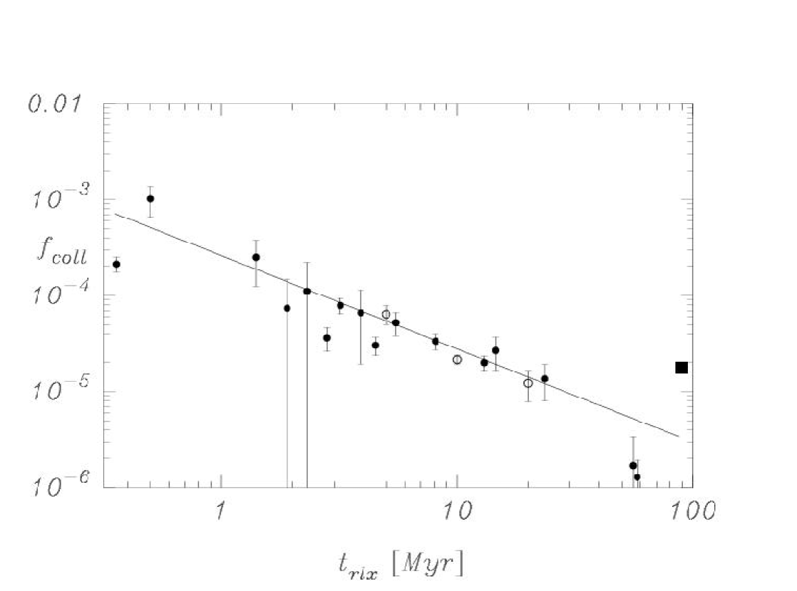
Figure 18: Mean collision rate $\mbox{${\rm f}_{\rm coll}$}={\mbox{$N_{\rm coll}$}/N\mbox{${t_{\rm last}}$}}$ as function of initial relaxation time for the simulations performed by Portegies Zwart et al. 1999; 2004 and Portegies Zwart & McMillan 2002). Here ${t_{\rm last}}$  is the time of the last collision in the cluster. The open circles give the results of systems which are isolated from the Galactic potential (see Portegies Zwart et al 1999). Vertical bars represent Poissonian 1-$\sigma$ errors. The solid line is a least squares fit to the data (see Eq. 42). The strong reduction in the collision rate for cluster with an initial relaxation time $\mbox{${t_{\rm rt}}$}\ {\raise-2.15277pt\hbox{$\buildrel>\over{\sim}$}}\ 30$ Myr is probably real. Note however the filled square to the right from the calculations of Portegies Zwart et al (2004), which gives a higher collision rate due to the high initial concentration of the models and the top-heavy mass function.

The number of collisions in the direct N-body  simulations ranged from 0 to 100. Fig. 18 shows the mean collision rate ${\cal N}_{\rm coll}$ per star per million years as a function of the initial half-mass relaxation time. The solid line in Fig. 18 is a fit to the simulation data, and has

$$\mbox{${\cal N}_{\rm coll}$}=2.2\times 10^{-4}{N\over\mbox{${t_{\rm rt}}$}}\,,$$ (42)

for $\mbox{${t_{\rm rt}}$}\ {\raise-2.15277pt\hbox{$\buildrel<\over{\sim}$}}\ 20-30$ Myr, consistent with our earlier estimate (Eq. 32) if $f_{\rm c}=0.2$. The quality of the fit in Fig. 18 is quite striking, especially when one bears in mind the rather large spread in initial conditions for the various models. See however the prominent square to the right, which is about a factor $\sim 3$ above the fitted curve. This discrepancy is mainly caused by the high average stellar mass in these models and by the use of much more concentrated King models.

The collision runaway phase lasts until about 3.3 Myr, at which time the designated target tends to collapse to a black hole.

In fig. 19 we present the cumulative distribution of the number of mergers of some of the calculations by Portegies Zwart et al (2004).

a)

b)

Figure 19: Cumulative distributions of the number of mergers which occurred within time $t$. Panel a) gives the results of the calculations performed with starlab, panel b) is from NBODY4. The dotted, solid and dashed curves are for the models with $W_{0}=8$ (in the right panel we show the results for $W_{0}=7$), $W_{0}=9$ and $W_{0}=12$. The dash-3-dotted curve in panel a) is for a model with $W_{0}=12$ with 10% primordial binaries. The dash-3-dotted curve in panel b) is for a model with $W_{0}=9$ using 585 000 stars, distributed according to a Kroupa (2001) initial mass function between 0.1 ${\rm M}_{\odot}$and 100 ${\rm M}_{\odot}$.

Figure 20 shows the cumulative mass distributions of the primary (more massive) and secondary (less massive) stars participating in collisions. We include only events in which the secondary experienced its first collision (that is, we omit secondaries which were themselves collision products). In addition, we distinguish between collisions early in the evolution of the cluster and those that happened later by subdividing our data based on the ratio $\tau=\mbox{${t_{\rm coll}}$}/{\mbox{${t_{\rm df}}$}}$, where ${t_{\rm coll}}$ is the time at which a collision occurred and ${t_{\rm df}}$ is the dynamical friction time scale of the secondary star (see Eq. 21). The solid lines in Figure 20 show cuts in the secondary masses at $\tau\ {\raise-2.15277pt\hbox{$\buildrel<\over{\sim}$}}\ 1$, $\tau\ {\raise-2.15277pt\hbox{$\buildrel<\over{\sim}$}}\ 5$ and $\tau<\infty$ (rightmost line). The mean secondary masses are $\mbox{${\langle m\rangle}$}=4.0\pm 4.8$ ${\rm M}_{\odot}$, $8.2\pm 6.5$ and $\mbox{${\langle m\rangle}$}=13.5\pm 8.8$ ${\rm M}_{\odot}$  for $\tau\ {\raise-2.15277pt\hbox{$\buildrel<\over{\sim}$}}\ 1$, 5 and $\infty$, respectively.

The distribution of primary masses in Figure 20 (dashed line) hardly changes as we vary the selection on $\tau$. We therefore show only the full ($\tau\ {\raise-2.15277pt\hbox{$\buildrel<\over{\sim}$}}\ \infty$) data set for the primaries. In contrast, the distribution of secondary masses changes considerably with increasing $\tau$. For small $\tau$, secondaries are drawn primarily from low-mass stars. As $\tau$ increases, the secondary distribution shifts to higher masses while the low-mass part of the distribution remains largely unchanged. The shift from low-mass ($\ {\raise-2.15277pt\hbox{$\buildrel<\over{\sim}$}}\ 8$ ${\rm M}_{\odot}$) to high-mass collision secondaries ($\ {\raise-2.15277pt\hbox{$\buildrel>\over{\sim}$}}\ 8$ ${\rm M}_{\odot}$) occurs between $\tau=1$ and $\tau=5$. This is consistent with the theoretical arguments presented in Sec. 3.1.2. During the early evolution of the cluster ($\tau\ {\raise-2.15277pt\hbox{$\buildrel<\over{\sim}$}}\ 1$), collision partners are selected more or less randomly from the available (initial) population in the cluster core; at later times, most secondaries are drawn from the mass-segregated population.

Interestingly, although hard to see in Fig. 20, all the curves are well fit by power laws between $\sim 8$ ${\rm M}_{\odot}$  and $\sim 80$ ${\rm M}_{\odot}$(0.8 ${\rm M}_{\odot}$  and 30 ${\rm M}_{\odot}$for the leftmost curve). The power-law exponents are $-0.4$, $-0.5$ and $-2.3$ for $\tau\ {\raise-2.15277pt\hbox{$\buildrel<\over{\sim}$}}\ 1$, 5, and $\infty$, and $-0.3$ for the primary (dashed) curve. (Note that the Salpeter mass function has exponent $-2.35$.)

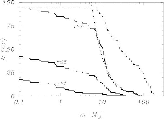
Figure 20: Cumulative mass distributions of primary (dashed line) and secondary (solid lines) stars involved in collisions. Only those secondaries experiencing their first collision are included. From left to right, the solid lines represent secondary stars for which $\tau\equiv\mbox{${t_{\rm coll}}$}/{\mbox{${t_{\rm df}}$}}\ {\raise-2.15277pt\hbox{$\buildrel<\over{\sim}$}}\ 1$, 5, and $\infty$. The numbers of collisions included in each curve are 18 (for $\mbox{${t_{\rm coll}}$}/{\mbox{${t_{\rm df}}$}}\ {\raise-2.15277pt\hbox{$\buildrel<\over{\sim}$}}\ 1$), 42 and 95 (rightmost two curves). The dotted line gives a power-law fit with the Salpeter exponent (between 5 ${\rm M}_{\odot}$  and 100 ${\rm M}_{\odot}$) to the right most solid curve ($\tau\ {\raise-2.15277pt\hbox{$\buildrel<\over{\sim}$}}\ \infty$).

Figure 17 shows the maximum mass reached by the runaway collision product as function of the initial mass of the star cluster. Only the left side ($\log M/\mbox{${\rm M}_{\odot}$}\ {\raise-2.15277pt\hbox{$\buildrel<\over{\sim}$}}\ 7$) of the figure is relevant here; we discuss the extrapolation to larger masses in Sec. 4.2. The N-body results are consistent with the theoretical model presented in Eq. 39.

3.3 Simulating the star cluster MGG11

In a recent publication (Portegies Zwart et al, 2004) we simulate a well observed star cluster in the starburst Galaxy M82. Interestingly enough, this cluster has experienced a prominent phase A evolution, and is currently in a phase B. In this §  I will report some of the interesting results about these simulations. Note that we have been quoting these results in earlier occasions in the text, but here we review the global results.

The observed mass function, as reported by McCrady et al (2003) for the M82 star cluster MGG11 is consistent with a Salpeter power-law (with $x=-2.35$) between 1 ${\rm M}_{\odot}$  and an upper limit which corresponds to the age of the cluster of 7 to 12 Myr. By that time all stars more massive than 17–25 ${\rm M}_{\odot}$  have experienced a supernova. For the IMF we adopt the same Salpeter slope and lower mass limit of 1 ${\rm M}_{\odot}$, but extend the upper limit to 100 ${\rm M}_{\odot}$. This IMF has an average mass of $\langle m\rangle\simeq 3.1\,M_{\odot}$. If we assume that at an age of 12–7 Myr all stars between 17–25 ${\rm M}_{\odot}$  and 100 ${\rm M}_{\odot}$  are lost from the cluster by supernova explosions, the mean stellar mass drops to $\langle m\rangle\simeq 2.4-2.6\,M_{\odot}$. With a current total mass of $3.5\times 10^{5}$ ${\rm M}_{\odot}$  the cluster would contain 130 000 to 140 000 stars. For clarity we decided to select 128k (131072) single stars, resulting in an initial mass of about 406,000 ${\rm M}_{\odot}$.

McCrady et al  (2003) measured the projected half light radius of the cluster, $r_{\rm hp}=1.2$ pc. De-projection of the half light radius depends on the density profile. For King (1966) models in the range $W_{0}=3-12$ it turns out that $r_{\rm h}=0.75-0.88r_{\rm hp}$ (which is somewhat larger than Spitzer’s, 1987 $r_{\rm h}\sim{3\over 4}r_{\rm hp}$). A number of initial test simulations indicate that over a time span of 7–12 Myr the projected half light radius of the selected IMF and number of stars, the cluster expands by about a factor 1.3. We then adopt an initial half mass radius for our models cluster of $r_{\rm hm}=1.2$ pc.

We ignore the effect of the tidal field of M82. The star cluster is located at a distance of about 160 pc from the dynamical center of the Galaxy, assuming a distance of 3.6 Mpc (Freedman et al. 1994). With the relatively small mass of M82 of $\sim 10^{9}$ ${\rm M}_{\odot}$  the gravitational force of the Galaxy is negligible compared to the self gravity of the stars within the cluster.

We performed several calculations starting from King models with different central concentrations $W_{0}$. We also performed one run with 10 per cent primordial binaries and one run starting with 585 000 stars and a Salpeter IMF between 0.1 ${\rm M}_{\odot}$  and 100 ${\rm M}_{\odot}$.

Table 4: Resulting collisions for our model clusters as a function of the initial density profile expressed in the King parameter $W_{0}$ (identified on the first column) and the average core density is presented in the second column. The third column gives the number of collisions which occurred in 12 Myr. The fourth and fifth columns give the number of collisions in which one particular star participates and the average mass of the star with which it collides. The last three columns give the number of collision and the mean mass of the more massive and lower mass stars participating in these collisions.

		designated target		other stars
$W_{0}$	$\rho_{c}$	$n_{\rm coll}$	$n_{\rm coll}$	$\langle m\rangle$	$n_{\rm coll}$	$\langle m\rangle$
	${\rm M}_{\odot}\,{\rm pc}^{-3}$	Results from Starlab
3	4.55	2	0	NA	2	17.3	5.0
7	5.51	5	0	NA	5	13.7	8.4
8	5.81	17	0	NA	17	19.0	9.7
9	6.58	36	21	48.1	15	16.4	6.2
12	8.12	27	14	47.9	12	33.2	9.0
12⋆		101	25	41.7	76	16.6	14.0
	Results from NBODY4
7		19	0	NA	19	24.7	4.6
9		164	99	30.0	65	34.8	8.1
12		98	70	38.7	28	50.1	7.8
9∘		161	98	20.9	63	31.5	3.1

^⋆: run performed with 10 per cent hard primordial binaries.
^∘: run performed with 585,000 stars and a Kroupa (2001) IMF between 0.1 ${\rm M}_{\odot}$and 100 ${\rm M}_{\odot}$  (for details see Portegies Zwart et al 2004).

To qualify the results we make the distinction between clusters with a high central concentration and clusters with low concentration. Since the initial half mass radius is the same for all models, we varied the density profile. For the density profile we adopted King (1966) models. We draw the empirical distinction between high concentration models having $W_{0}\ {\raise-2.15277pt\hbox{$\buildrel>\over{\sim}$}}\ 9$; low concentration models have $W_{0}\ {\raise-2.15277pt\hbox{$\buildrel<\over{\sim}$}}\ 8$. With the adopted half-mass radius and total mass the high concentration cluster $W_{0}\ {\raise-2.15277pt\hbox{$\buildrel>\over{\sim}$}}\ 9$ models have core density $\log\rho_{c}>6$ ${\rm M}_{\odot}$ pc^-3.

In figure 21 we present the evolution of the central density of various starlab models with $W_{0}=7$, 8 and 9. As discussed, in the low concentration models core collapse is arrested by the copious mass loss from the evolving massive stars. In the high concentration clusters core collapse occurs early enough that the process is little affected by stellar mass loss.

Figure 21: Evolution of the central density for star clusters with $W_{0}=7$ (dash-3-dotted line), $W_{0}=8$ (dahses), $W_{0}=9$ (dotted curve). The $W_{0}=9$ model shows a clear core collapse at about 0.7 Myr, indicated with the arrow. The less concentrated models ($W_{0}=8$ and $W_{0}=7$) show a very shallow start of a core collapse near $t\sim 3$ Myr, but in these cases the collapse of the core is arrested by stellar mass loss. In fig. 13 we present the evolution of the core radius for the same calculations.

3.3.1 Clusters with $\log\rho_{c}>6$ ${\rm M}_{\odot}$ pc^-3

According to Portegies Zwart et al (1999), who studied similar clusters as Portegies Zwart & McMillan (2002), the high collision rate is mainly the result of binaries created in 3-body encounters during core collapse. In our latest models, however, only about half ($0.52\pm 0.1$) the collisions are preceded by the formation of a binary, the other half are direct hits in which no third star was bound to the two stars which ultimately collided. Though seemingly a detail, it has far reaching consequences for the interpretation of the collisional growth which plays an important role in the evolution of these systems.

After the first epoch of runaway growth and the collapse of the designated target, an epoch of about 3 Myr starts in which the collision rate drops dramatically. This phase is visible in fig. 19 between $\sim 3.3$ Myr and $\sim 6$ Myr.

This quiet phase lasts until the first M5I hyper giants appear, which, in our stellar evolution model, happens at a turn-off mass of $\sim 25$ ${\rm M}_{\odot}$  (at $\sim 6$ Myr). (Note that in our stellar evolution model SeBa stars below $\sim 25$ ${\rm M}_{\odot}$  turn into neutron stars where more massive stars become black holes, see Portegies Zwart & Verbunt 1996) By this time the collision rate picks up again to 2-3 per Myr. The spectral type M0I – M5I star dominate the collision rate; the designated target, now an intermediate mass black hole, participates in only about one-third of the collisions. This phase lasts until about 9–12 Myr, after which the rate drops below 0.3 collisions per Myr.

3.3.2 Clusters with $\log\rho_{c}<6$ ${\rm M}_{\odot}$ pc^-3

In low density cluster $W_{0}\ {\raise-2.15277pt\hbox{$\buildrel<\over{\sim}$}}\ 8$ the initial phase of runaway growth is absent. The subsequent collisional phase at an age $\ {\raise-2.15277pt\hbox{$\buildrel>\over{\sim}$}}\ 6$ Myr, however, occurs at a comparable rate as in the high density simulations (see fig. 20). As discussed in the previous §  there is no designated target in this phase; all collisions tend to happen between massive stars (or stellar remnants) of which at least one component is evolved (spectral type M0I to M5I). At a rate which becomes gradually smaller for less concentrated clusters: 3.4 collisions per Myr for $W_{0}=9$, 3.2 for $W_{0}=8$, 1.6 for $W_{0}=7$, 1.5 for $W_{0}=5$ and 0.5 for $W_{0}=3$. Curiously enough the $W_{0}=12$ models have a collision rate of only 2.3 per Myr, which is lower than the less concentrated $W_{0}=9$ models.

The average star with which a collision occurs (counting the least massive of the two stars) depends on the initial cluster density profile, ranging from a 5.3 ${\rm M}_{\odot}$  for $W_{0}=5$, 6.2 ${\rm M}_{\odot}$  for $W_{0}=7$, 9.7 ${\rm M}_{\odot}$  for $W_{0}=8$ and $\sim 30$ for both $W_{0}=9$ and $W_{0}=12$ (consistent with the expectations of Portegies Zwart & McMillan 2002)

3.4 Black hole ejection in phase B and C cluster with $\mbox{${t_{\rm rt}}$}\ {\raise-2.15277pt\hbox{$\buildrel>\over{\sim}$}}\ 100$ Myr

Here we discuss the evolution of star clusters in which the early phase is dominated by stellar mass loss and the subsequent evolution by the stellar interaction; $\tau_{\rm SE}<\tau_{\rm SD}$. In this regime or parameter space, the most massive stars evolve before the structure of the star cluster has appreciably changed, i.e; no intermediate mass black hole can form via the scenario discussed in § 3.1. The consequence is that the most massive stars turn into black holes and neutron stars before they had a chance to sink to the cluster center by dynamical friction. This regime is valid for most globular clusters, and possibly many open star clusters.

Upon the birth of a cluster we assume that the stars populate the initial mass function from the hydrogen burning limit ($\sim 0.1$ ${\rm M}_{\odot}$) all the way to the most massive stars currently observed in the Galaxy, which is about 100 ${\rm M}_{\odot}$. Stars with Solar abundance between 50 ${\rm M}_{\odot}$  and 100 ${\rm M}_{\odot}$  leave the main sequence at an age of about 3.7 Myr to 3.3 Myr, to explode in a supernova a few hundred thousand years later. The total mass in this range is about 1%, and the cluster therefore loses approximately 1% of its total mass in less than half a million years.

The first black holes are produced at about the same time. Black hole formation proceeds to about 7–9 Myr, until all stars with initial masses exceeding 20–25 ${\rm M}_{\odot}$(Maeder 1992; Portegies Zwart et al. 1997). have collapsed to black holes. Assuming a Scalo (1986) mass distribution with a lower mass limit of 0.1 ${\rm M}_{\odot}$  and an upper limit of 100 ${\rm M}_{\odot}$  about 0.071% of the stars are more massive than 20 ${\rm M}_{\odot}$, and 0.045% are more massive than 25 ${\rm M}_{\odot}$. A star cluster containing $N$ stars thus produces $\sim 6\times 10^{-4}N$ black holes. Known Galactic black holes have masses ${m_{\rm bh}}$ between 6 ${\rm M}_{\odot}$  and 18 ${\rm M}_{\odot}$ (Timmes et al.  1996). For definiteness, we adopt $\mbox{${m_{\rm bh}}$}=10$ ${\rm M}_{\odot}$.

A black hole is formed in a supernova explosion. If the progenitor is a single star (i.e. not a member of a binary), the black hole experiences little or no recoil and remains a member of the parent cluster (White & van Paradijs 1996). If the progenitor is a member of a binary, mass loss during the supernova may eject the binary from the cluster potential via the Blaauw mechanism (Blaauw 1961), where conservation of momentum causes recoil in a binary as it loses mass impulsively from one component. The Blaauw velocity kick can be as large as the relative orbital velocity of the pre-supernova binary (see e.g.  Nelemans et al (2001). The escape speed is $\sim 40\,$${\rm km~{}s}^{-1}$for a young globular cluster, and somewhat smaller for YoDeCs (see Tab 1). Such high recoil velocities are generally achieved only if the binary loses $\ {\raise-2.15277pt\hbox{$\buildrel<\over{\sim}$}}\ 50$% of its total mass in the supernova, and if its orbital period is initially quite small ($\ {\raise-2.15277pt\hbox{$\buildrel<\over{\sim}$}}\ 2$ yr) (Portegies Zwart & Verbunt 1996). The binary frequency in globular clusters is between 5 and 40% (Rubenstein 1997), and less than 30% of binaries have orbital periods smaller than 2 years (Rubenstein & Bailyn 1997; 1999); we assume the same distributions of orbital parameters for binaries in YoDeCs. We therefore estimate that no more than $\sim 10$% of black holes are ejected from the cluster immediately following their formation (i.e. the black hole retention fraction is $\ {\raise-2.15277pt\hbox{$\buildrel>\over{\sim}$}}\ 90$%). Note the remarkable difference here with the retention fraction of neutron stars, which is less than about 10% (Drukier 1996).

After $\sim 40$ Myr the last supernova has occurred, the mean mass of the cluster stars is $\mbox{${\langle m\rangle}$}\sim 0.56$ ${\rm M}_{\odot}$ (Scalo 1986), and black holes are by far the most massive objects in the system. Mass segregation cause the black holes to sink to the cluster core in a fraction $\sim\mbox{${\langle m\rangle}$}/\mbox{${m_{\rm bh}}$}$ of the half-mass relaxation time scale (see Eq. 21). For a young populous cluster, the relaxation time is on the order of 10 Myr; for a globular cluster it is about 1 Gyr (see Tab. 3).

By the time of the last supernova, stellar mass loss has also significantly diminished and the cluster core starts to contract, enhancing the formation of binaries by three-body interactions. Single black holes form binaries preferentially with other black holes (Kulkarni et al. 1993), while black holes born in binaries with a lower-mass stellar companion rapidly exchange the companion for another black hole. The result in all cases is a growing black-hole binary population in the cluster core. Once formed, the black-hole binaries become more tightly bound through superelastic encounters with other cluster members (Heggie 1975; Kulkarni et al. 1993; Sigurdsson & Hernquist 1993). On average, following each close binary–single black hole encounter, the binding energy of the binary increases by about 20% (Hut et al. 1992); roughly one third of this energy goes into binary recoil, assuming equal mass stars. The minimum binding energy of an escaping black-hole binary may then be estimated as

$$E_{b,{\rm min}}\sim 36\,W_{0}\,\frac{\mbox{${m_{\rm bh}}$}}{\mbox{${\langle m\rangle}$}}\,kT\,,$$ (43)

where $\frac{3}{2}kT$ is the mean stellar kinetic energy and $W_{0}=\mbox{${\langle m\rangle}$}|\phi_{0}|/kT$ is the dimensionless central potential of the cluster (King 1966). By the time the black holes are ejected, $\mbox{${\langle m\rangle}$}\sim 0.4\,\mbox{${\rm M}_{\odot}$}$. Taking $W_{0}\sim 10$ we find $E_{b,{\rm min}}\sim 10000\,kT$.

Portegies Zwart & McMillan (2000) have tested and refined the above estimates by performing a series of N-body  simulations within the Starlab software environment using the special-purpose computer GRAPE-4 to speed up the calculations (see § 1.4.4). For most (seven) of these calculations we used 2048 equal-mass stars with 1% of them ten times more massive than the average; two calculations were performed with 4096 stars. One of the 4096-particle runs contained 0.5% black holes; the smaller black-hole fraction did not result in significantly different behavior. They also tested alternative initial configurations, starting some models with the black holes in primordial binaries with other black holes, or in primordial binaries with lower-mass stars.

The results of these simulations may be summarized as follows. Of a total of 204 black holes, 62 ($\sim 30\%$) were ejected from the model clusters in the form of black-hole binaries. A total of 124 ($\sim 61\%$) black holes were ejected single, and one escaping black hole had a low-mass star as a companion. The remaining 17 ($\sim 8\%$) black holes were retained by their parent clusters. The binding energies $E_{b}$ of the ejected black-hole binaries ranged from about $1000\,kT$ to $10000\,kT$ in a distribution more or less flat in $\log E_{b}$, consistent with the assumptions made by Hut et al. (1992). The eccentricities $e$ followed a roughly thermal distribution [$p(e)\sim 2e$], with high eccentricities slightly overrepresented; the mean eccentricity was $\langle e\rangle=0.69\pm 0.10$. The 17 binaries with the lowest binding energies ($\log_{10}E_{b}<3.5$) had on average higher eccentricities ($\langle e\rangle=0.78\pm 0.05$) than the more tightly bound binaries ($\langle e\rangle=0.62\pm 0.11$). About half of the black holes were ejected while the parent cluster still retained more than 90% of its birth mass, and $\ {\raise-2.15277pt\hbox{$\buildrel>\over{\sim}$}}\ 90$% of the black holes were ejected before the cluster had lost 30% of its initial mass. These findings are in good agreement with previous estimates that black-hole binaries are ejected within a few Gyr, well before core collapse occurs (Kulkarni et al. 1993; Sigurdsson & Hernquist 1993). Recently Merritt et al.  (2004) confirmed these findings with their own simulations using NBODY6++, (Hemsendorf et al 2002; and can be downloaded from ftp://ftp.ari.uni-heidelberg.de/pub/staff/spurzem/nb6mpi/ a parallel version of NBODY6 (Aarseth 1999).

Portegies Zwart & McMillan (2000) have performed additional calculations incorporating a realistic (Scalo 1986) mass function, the effects of stellar evolution, and the gravitational influence of the Galaxy. These model clusters generally dissolved rather quickly (within a few hundred Myr) in the Galactic tidal field. We found that clusters which dissolved within $\sim 40$ Myr (before the last supernova) had no time to eject their black holes; however, those that survived for longer than this time were generally able to eject at least one close black-hole binary before dissolution.

Based on these considerations, we conservatively estimate the number of ejected black-hole binaries to be about $10^{-4}N$ per star cluster, more or less independent of the cluster lifetime.

3.4.1 Characteristics of the black-hole binary population

The energy of an ejected binary and its orbital separation are coupled to the dynamical characteristics of the star cluster. For a cluster in virial equilibrium, we have

$$kT=\frac{2E_{\rm kin}}{3N}=\frac{-E_{\rm pot}}{3N}={GM^{2}\over 6N\mbox{${r_{\rm vir}}$}}\,,$$ (44)

where $M$ is the total cluster mass and ${r_{\rm vir}}$ is the virial radius. A black-hole binary with semi-major axis $a$ has

$$E_{b}={Gm_{\rm bh}^{2}\over 2a},$$ (45)

and therefore

$${E_{b}\over kT}=3N\left({m_{\rm bh}\over M}\right)^{2}{\mbox{${r_{\rm vir}}$}\over a}.$$ (46)

In computing the properties of the black-hole binaries resulting from cluster evolution, it is convenient to distinguish three broad categories of dense stellar systems: (1) YoDeCs, (2) globular clusters, and (3) galactic nuclei. Table 1 lists characteristic parameters for each category. The masses and virial radii of globular clusters are assumed to be distributed as independent Gaussian with means and dispersions as presented in the table; this assumption is supported by correlation studies (Djorgovski & Meylan 1994). Table 1 also gives estimates of the parameters of globular clusters at birth (bottom row), based on a recent parameter-space survey of cluster initial conditions (Takahashi & Portegies Zwart 2000; Baumgardt & Makino 2003); globular clusters which have survived for a Hubble time have lost $\ {\raise-2.15277pt\hbox{$\buildrel>\over{\sim}$}}\ 60$% of their initial mass and have expanded by about a factor of three. We draw no distinction between core-collapsed globular clusters (about 20% of the current population) and non-collapsed globulars—the present dynamical state of a cluster has little bearing on how black-hole binaries were formed and ejected during the first few Gyr of the cluster’s life.

The above described process causes globular clusters to be depleted of black holes. At most one binary containing two black holes can be present in any globular cluster. In § 4.4 we will further discuss the consequences of the ejected black holes and black hole binaries, as the latter may become important sources for gravitational wave detectors.

4 Discussion and further speculations

Now we have discussed the basic principles of star cluster dynamics with black holes. In this section we further discuss some of the consequences and observables to which this theory can be tested.

4.1 Turning an intermediate mass black hole in an X-ray source

An IMBH in a stellar cluster with velocity dispersion $\sigma$ dominates the potential well within its radius of influence $R_{\rm i}=G\mbox{${m_{\rm bh}}$}/\sigma^{2}$; inside $R_{\rm i}$ the orbits are approximately Keplerian, and the stars are distributed according to a power law (see Eq. 2.1.1 and also (Bahcall & Wolf). N-body calculations show that $\alpha=1.5$ (Baumgardt et al 2004), and we assume this value in the following.

Stars can reach an orbit with peribothron of order of the tidal radius by energy diffusion or by angular momentum diffusion. However, stellar collisions become the dominant dynamical process within the collision radius $r_{\mathrm{coll}}\sim(\mbox{${m_{\rm bh}}$}/m)r$ (Frank & Rees 1976), disrupting stars within that region, and making energy diffusion within $r_{\mathrm{coll}}$ implausible. For this reason we concentrate on tidal capture of stars on very eccentric orbits. When the star arrives at peribothron a certain amount of energy $\Delta E_{t}$ is invested in raising tides, causing the orbit to circularize. It is hard to know how the star dissipates the tides after the repetitive encounters with the IMBH. Two extreme models of “squeezars” (stars that are “squeezed” by the tidal field) are studied by Alexander & Morris (2003), namely “cold squeezars”, which puff up, or “hot squeezars”, which are heated only in their outer layers and radiate their excess energy effectively.

Hopman et al (2003) calculated that the probability that an intermediate mass black hole captures a stellar companion via this process (assuming the “hot squeezar” model) has a reasonable probability, making it likely that we could in fact observe one or two of such objects. Once captured the companion star is likely to fill its Roche-lobe while still on the main-sequence.

From the moment of first Roche-lobe contact the evolution of the binary is further determined by mass transfer from a lower mass (secondary) star to the much more massive (primary) IMBH. This process is driven by the thermal expansion of the donor and the loss of angular momentum from the binary system. Mass transfer then implies that the donor fills its Roche lobe ($R_{\rm don}=R_{\rm Rl}$) and continues to do so, i.e., $\mbox{$\dot{R}$}_{\rm don}=\mbox{$\dot{R}$}_{\rm Rl}$. We also assume that, as long as $L_{\rm disc}<L_{\rm Edd}$ all the mass lost from the donor via the Roche lobe is accreted by the black hole, $\mbox{$\dot{M}$}=-\mbox{$\dot{m}$}$. If the mass transfer rate exceeds the Eddington limit, the remaining mass is lost from the binary system with the angular momentum of the accreting star.

We estimate the X-ray Luminosity during mass transfer using the simple model of Körding, Falcke & Markoff (2002). They argue that in the hard state ($\mbox{$\dot{m}$}>\mbox{$\dot{m}_{\rm crit}$}$) $L_{x}\simeq 0.1\mbox{$\dot{m}$}c^{2}$, where at lower accretion rates the source becomes transient (see also Kalogera et al, 2004) with an average luminosity of $L_{x}\simeq 0.1c^{2}\mbox{$\dot{m}$}^{2}/\mbox{$\dot{m}_{\rm crit}$}$. For $\dot{m}_{\rm crit}$  we use the relation derived by Dubus et al (1999)

Figure 22: Estimated X-ray luminosity (log erg/s) as a function of time for a $1000\,\mbox{${\rm M}_{\odot}$}\,$ accreting black hole. The solid, dashed and dotted curves are for a $15\,\mbox{${\rm M}_{\odot}$},10\,\mbox{${\rm M}_{\odot}$}\,$ and a $5\,\mbox{${\rm M}_{\odot}$}\,$ donor which started Roche-lobe overflow at the zero-age main-sequence. (Figure from Hopman, Portegies Zwart & Alexander, 2004)

4.2 Speculation on the formation of supermassive black holes

A million-solar-mass star cluster formed at a distance of $\ {\raise-2.15277pt\hbox{$\buildrel<\over{\sim}$}}\ 30$ pc from the Galactic center can spiral into the Galactic center by dynamical friction before being disrupted by the tidal field of the Galaxy (see Gerhard 2001). Only the densest star clusters survive to reach the center. These clusters are prone to runaway growth and produce massive compact objects at their centers. Upon arrival at the Galactic center, the star cluster dissolves, depositing its central black hole there. Black holes from in-spiraling star clusters may subsequently merge to form a supermassive black hole. Ebisuzaki et al. (2001) have proposed that such a scenario might explain the presence of the central black hole in the Milky way galaxy.

If we simply assume that bulges and central supermassive black holes are formed from disrupted star clusters, this model predicts a relation between black hole and bulge masses in galaxies similar to the expression (Eq. 40) connecting the mass of an IMBH to that of its parent cluster. However, the ratio of stellar mass to black-hole mass might be expected to be smaller for galactic bulges than for star clusters, because not all star clusters produce a black hole and not all star clusters survive until the maximum black hole mass is reached. We would expect, however, that the general relation between the black hole mass and that of the bulge remains valid.

Figure 17 shows the relation between the black hole mass and the bulge mass for several Seyfert galaxies and quasars. The expression derived in Sec. 3.1.3 and the results of these N-body  calculations (Sec. 3.2) are also indicated. The solid and dashed lines (Eq. 40) fit the N-body  calculations and enclose the area of the measured black hole mass–bulge masses. On the way, the solid curve passes though the two black-hole mass estimates, for M82 star cluster MGG-11. We note that the observed relation between bulge and black hole masses has a spread of two orders of magnitude. If this bold extrapolation really does reflect the formation process of bulges and central black holes, this spread could be interpreted as a variation in the efficiency of the runaway merger process. In that case, only about one in a hundred star clusters reaches the galactic center, where its black hole is deposited.

The dashed curve is an extrapolation beyond $10^{7}$ ${\rm M}_{\odot}$  the range where we think that Eq. 40 is applicable. There appears to be a very interesting relation for galactic nuclei between the velocity dispersion and the mass of the central black hole (Ferrarese & Merritt 2000; Gebhardt et al 2000, 2001); and Merritt & Ferrarese (2001). I do not wish to claim that the process described in Eq. 40 and the formation of supermassive black holes in galactic nuclei (see however Ebisuzaki et al 2001), but just point out how well the same theory explains the relation between nuclear black hole mass and the velocity dispersion in the nucleus. At the moment of writing there more than a dozen alternative explanations for this interesting relation (see for example Haehnelt et al.  2000; Dokushaev et al 2002; Boroson et al 2002); Green et al (2004);), and this number is growing almost daily.

4.3 Is the globular cluster M15 a special case?

The presence of an intermediate mass black hole in the core collapsed globular cluster M15 has been vividly debated over the last several decades (Illingworth & King, 1977a, 1977b) and is still discussed to the present day (van der Marel et al 2002). If M15 contains an intermediate mass black hole, as has recently been suggested by some observers (Gerrisen et al, 2002; later retracted and subsequently corrected in Gerrisen 2003) and argued against by theorists (Baumgardt et al 2003), it is unlikely to have formed via the scenario discussed in § 3.1. The cluster’s initial relaxation time probably exceeded our upper limit of $\sim 100$ Myr. The current half-mass relaxation time of M15 is about 2.5 Gyr (Harris 1996), which is far more than our 100 Myr limit for forming a massive central object from a collision runaway (see § 3.1 for details).

An intermediate mass black hole in the globular cluster M15 may have been formed by a different scenario. An alternative is provided by Miller & Hamilton (2001), who describe the formation of massive ($\sim 10^{3}$ ${\rm M}_{\odot}$) black holes in star clusters with relatively long relaxation times. In their model the black hole grows very slowly over a Hubble time via occasional collisions with other black holes, in contrast to the model described here, in which the runaway grows much more rapidly, reaching a characteristic mass of about 0.1% of the total birth mass of the cluster within a few megayears.

One possible way around M15’s long relaxation time may involve the cluster’s rotation. Gebhardt (2000; 2001; private communication) has measured radial velocities of individual stars in the crowded central field, down to two arcsec of the cluster center. He finds that, both in the central part of the cluster ($R<0.1R_{\rm hm}$) and outside the half mass radius, the average rotation velocity is substantial ($\mbox{$v_{\rm rot}$}\ {\raise-2.15277pt\hbox{$\buildrel>\over{\sim}$}}\ 0.5\mbox{$\langle v\rangle$}$). Rotation is quickly lost in a cluster (Baumgardt et al 2003), so to explain a current rotation, M15’s initial rotation rate must probably have been even larger than observed today (see Einsel & Spurzem 1999). Hachisu (1978; 1982) found, using gaseous cluster models, that an initially rotating cluster tends to evolve into a ’gravo-gyro catastrophe’ which drives the cluster into core collapse far more rapidly than would occur in a non-rotating system. If the gravo-gyro-driven core collapse occurred within 25 Myr, a collision runaway might have initiated the growth of an intermediate mass black hole in the core of M15.

4.4 The gravitational wave signature of dense star clusters

The peak amplitude of the gravitational wave form produced by black-hole inspiral is (Peters 1964)

$$h=8.0\times 10^{-20}\left({M_{\rm chirp}\over\mbox{${\rm M}_{\odot}$}}\right)^{5/6}\left({20\,{\rm ms}\over P_{\rm orb}}\right)^{1/6}\left({1{\rm Mpc}\over d}\right)\,.$$ (47)

Here the “chirp” mass is $M_{\rm chirp}=(m_{1}m_{2})^{3/5}/(m_{1}+m_{2})^{1/5}$ for a binary with component masses $m_{1}$ and $m_{2}$. The frequency of the gravitational wave is $2/P_{\rm orb}$, where $P_{\rm orb}$ is the orbital period. The first LIGO interferometer is expected to achieve a sensitivity $h$ of $10^{-20}$ to $10^{-21}$ at its most sensitive frequency around 100 Hz (Abramovici et al.  1992), corresponding to an orbital period of about 20 ms. The details of the wave form and the recovery of the signal from the noisy data complicates matters somewhat. With a sensitivity of $h=5\times 10^{-21}$, black-hole binaries will be detectable out to a distance of about 100 Mpc, and intermediate mass black holes to several kpc distances. Within a volume of $\frac{4}{3}\pi d^{3}$ we then expect a detection rate for the first generation of interferometers of about 0.3 $h_{0}^{3}$ per year. For $h_{0}\sim 0.72$ (Freedman et al. 2001), this results in about one detection event per decade. LIGO-II is tentatively expected to see out to an effective distance about ten times farther than LIGO-I and be operational between 2005 to 2007 (K. Thorne, private communication). This would result in a 1000 times higher detection rate, or several events per month.

The current best estimate of the maximum distance within which LIGO-I can detect an inspiral event is

$$R_{\rm eff}=18\,{\rm Mpc}\ \left(\frac{M_{\rm chirp}}{\mbox{${\rm M}_{\odot}$}}\right)^{5/6}$$ (48)

(K. Thorne, private communication). For neutron star inspiral, $m_{1}=m_{2}=1.4\,\mbox{${\rm M}_{\odot}$}$, so $M_{\rm chirp}=1.22\,\mbox{${\rm M}_{\odot}$}$, $R_{\rm eff}=21$ Mpc. For black-hole binaries with $m_{1}=m_{2}=\mbox{${m_{\rm bh}}$}=10\,\mbox{${\rm M}_{\odot}$}$, we find $M_{\rm chirp}=8.71\,\mbox{${\rm M}_{\odot}$}$, $R_{\rm eff}=109$ Mpc.

4.4.1 The gravitational wave signature for intermediate mass black holes

In § 4.1 we discussed a model for producing X-rays from an intermediate mass black hole, in this §  we continue that discussion but then in relation to gravitational wave detectors.

Figure 23: A selected sample of binaries in the gravitational wave strain and frequency domain with the LISA and LIGO noise curves over-plotted. We assumed a distance to the source of 10kpc. The lower solid curve to the right is for a 2 ${\rm M}_{\odot}$  donor, the dashes for a 5 ${\rm M}_{\odot}$  donor, the dotted curves are for a 10 ${\rm M}_{\odot}$  donor with a 100 ${\rm M}_{\odot}$  black hole (lower dotted curve) and 1000 ${\rm M}_{\odot}$  black hole (upper dotted curve). The upper solid curve is for a 15 ${\rm M}_{\odot}$  donor. Except for the lower dotted curve are all calculations for a 1000 ${\rm M}_{\odot}$  donor. Notice the enormous difference for the 2 ${\rm M}_{\odot}$  donor, which is caused by the lack of growth in size of the donor.

Figure 23 presents the evolution of the gravitational wave signal for several systems which start mass transfer at zero age. Assuming a standard distance of 10 Kpc, the binaries which start mass transfer at birth emit gravitational waves at a strain of about $\log h\simeq-20.2$ (almost independent of the donor mass). The frequency of the gravitational waves is barely detectable for the LISA space based antennae (see Figure 23). During mass transfer the binary moves out of the detectable frequency band, as the orbital period increases. Once the donors has turned into a white dwarf, as happens for the 5 ${\rm M}_{\odot}$  and 10 ${\rm M}_{\odot}$  donors, the emission of gravitational waves brings the two stars back into the relatively high frequency regime and it becomes detectable again for the LISA antennae. This process, however takes far longer than a Hubble time.

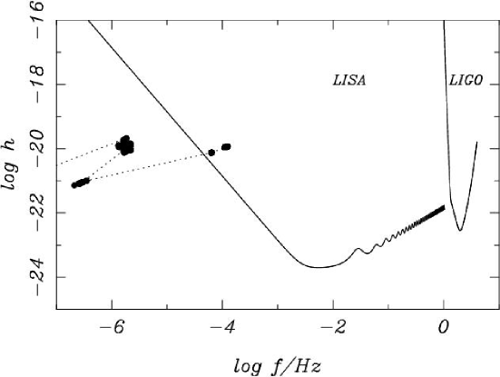
Figure 24: Evolutionary track in gravitational wave space (frequency and strain) for an intermediate mass black hole formed in a young and dense star cluster at a distance of 1kpc. the initial conditions were to mimic the M82 star cluster MGG-11 (Portegies Zwart et al. 2004). The bullets indicate the moments of output one million years apart. They are connected with a dotted line. The intermediate mass black hole acquires a stellar mass black hole in a close binary near the end of the simulation at about 90 Myr which puts it in the LISA band.

The binary in which a 2 ${\rm M}_{\odot}$  main-sequence star starts to transfer to a 1000 ${\rm M}_{\odot}$  black hole, however, remains visible as a bright source of gravitational waves for its entire lifetime (see Figure 23). The reason for this striking result is the curious evolution of the donor as it transfers mass at a slow rate. The 2 ${\rm M}_{\odot}$  main-sequence donor becomes fully mixed after the hydrogen fraction exceed about 66 per cent. As a result, the star remains rather small in size and therefore the orbital period during mass transfer remains roughly constant. This binary remains visible in the LIGO frequency regime for its entire main-sequence lifetime, only the gravitational wave strain drops as the donor is slowly consumed by the intermediate mass black hole. Mass transfer in this evolution stage is rather slow causing the X-ray source to be transient. Such a transient could result in an interesting synchronous detection of X-rays and gravitational waves.

Figure 25: Population of compact stars in binaries in gravitational wave space (frequency and strain) in a simulated star cluster at a distance of 1kpc. The initial conditions were to mimic the M82 star cluster MGG-11 (Portegies Zwart et al. 2004). The cluster was 100 Myr when this image was taken. The bullets indicate binaries with one or two black holes, open circles indicate neutron stars and small dots are for white dwarfs. Where symbols overplot exactly, as is quite common for a circle with a small dot in the middle indicate close binaries with two different compact objects, in these cases they are (ns, wd) binaries. Only a few white dwarf binaries may be visible in the LISA band, black hole and neutron star binaries are generally too wide to be detectable. The intermediate mass black hole is not shown here, but in figure. 24.

The star cluster contains many of binaries, some of which may have orbital periods small enough, and component masses large enough to be visible by advanced gravitational wave detectors. In figure 25 we show the population of binaries in gravitational-wave space (strain $h$ versus frequency $f$) for the compact binaries for one of our MGG-11 simulations (see § 3.3) at an age of 100 Myr. This simulation model had initially 20% of its 128k stars in a binary system. The majority of systems is not even on this graph, as they comprise of main-sequence stars, giants or other ’large’ stellar object. Only binaries with at least one compact objects are presented, and of these only the white dwarf binaries make it in the LISA band. Many of these systems, however, will be unobservable in realistic star clusters, as the star cluster is much further than the here adopted 1 kpc or the system ends-up in the confusion limited noise of the white dwarf population from the Milky-way Galaxy (see e.g.  Hogan & Bender 2001; Seto 2002; Nelemans et al, 2004, but see Benaquista et al 2001).

4.4.2 The merger rate of stellar mass black holes

In § 3.4 we discussed the evolution of relatively low density clusters through phase B and C. These clusters tend to eject their lack holes, in part in the form of binaries consisting of two black holes. The orbital parameters of these binaries are such that merger may occur in a relatively short time scale; well withing a Hubble time. We now will discuss the merger rate per unit volume ${\cal R}$ which we predict from various types of star clusters.

A conservative estimate of the merger rate of black-hole binaries formed in globular clusters is obtained by assuming that globular clusters in other galaxies have characteristics similar to those found in our own. Using the galaxy density in the local universe (see Tab. 2) the result is

$${\cal R}_{GC}=5.4\times 10^{-8}h^{3}\;{\rm yr}^{-1}\,{\rm Mpc}^{-3}.$$ (49)

Irregular galaxies, starburst galaxies, early type spirals and blue elliptical galaxies all contribute to the formation of young dense clusters. In the absence of firm measurements of the numbers of YoDeCs in other galaxies, we simply use the same values of $S_{N}$ as for globular clusters (see from Tab. 2). The space density of such clusters is then

$$\phi_{\rm YoDeC}=3.5\,h^{3}\;{\rm Mpc^{-3}},$$ (50)

and the black hole merger rate is

$${\cal R}_{\rm YoDeC}=2.1\times 10^{-8}h^{3}\;{\rm yr}^{-1}\,{\rm Mpc}^{-3}.$$ (51)

For purposes of comparison, we also estimate the contribution to the total merger rate from galactic nuclei, neglecting obvious complicating factors such as the presence of central supermassive black holes (Sage 1994), which may inhibit the formation, hardening, and ejection of black-hole binaries. The space density of galactic nuclei is only about

$$\phi_{GN}=0.012\,h^{3}\;{\rm Mpc^{-3}},$$ (52)

and the corresponding contribution to the black hole merger rate is

$${\cal R}_{GN}=2.5\times 10^{-9}h^{3}\;{\rm yr}^{-1}\,{\rm Mpc}^{-3},$$ (53)

which is negligible compared to the other rates.

Based on the assumptions outlined above, our estimated total merger rate per unit volume of black-hole binaries is

$${\cal R}=7.5\times 10^{-8}h^{3}\;{\rm yr}^{-1}\,{\rm Mpc}^{-3}.$$ (54)

However, this may be a considerable underestimate of the true rate. First, as already mentioned, our assumed number ($\sim 10^{-4}N$) of ejected black-hole binaries is quite conservative. Second, the correlation between orbital eccentricity and binding energy and the excess of high-eccentricity binaries mentioned earlier both favor more rapid inspiral, causing a larger fraction of the black-hole binaries to merge. Third, the observed population of globular clusters naturally represents only those clusters that have survived until the present day. The study by Takahashi & Portegies Zwart (2000) and Baumgardt & Makino (2003) indicates that $\sim$ 50% of globular clusters dissolve in the tidal field of the parent galaxy within a few billion years of formation. We have therefore underestimated the total number of globular clusters, and hence the black-hole merger rate, by about a factor of two. Fourth, a very substantial underestimate stems from the assumption that the masses and radii of present-day globular clusters are representative of the initial population. When estimated initial parameters (Table 1, bottom row) are used, the total merger rate increases by a further factor of six. Taking all these effects into account, we obtain a net black-hole merger rate of

$${\cal R}\sim 6\times 10^{-7}h^{3}\;{\rm yr}^{-1}\,{\rm Mpc}^{-3}.$$ (55)

We note that this rate is significantly larger than the current best estimates of the neutron-star merger rate (e.g.  Phinney 1991; Tutukov & Yungelson 1994; Burgay et al. 2003; and many others). Since black hole mergers are also “visible” to much greater distances, we expect that black hole events will dominate the LIGO detection rate.

4.4.3 Gravitational inspiral

An approximate formula for the merger time of two stars due to the emission of gravitational waves is given by Peters (1964):

$$t_{\rm mrg}\approx 150\,{\rm Myr}\;\left({\mbox{${\rm M}_{\odot}$}\over\mbox{${m_{\rm bh}}$}}\right)^{3}\left({a\over\mbox{${\rm R}_{\odot}$}}\right)^{4}(1-e^{2})^{7/2}\;.$$ (56)

The sixth column of Table 1 lists the fraction of black-hole binaries which merge within a Hubble time due to gravitational radiation, assuming that the binary binding energies are distributed flat in $\log E_{b}$ between $1000\,kT$ and $10000\,kT$, that the eccentricities are thermal, independent of $E_{b}$, and that the universe is $\sim 13$ Gyr old ($H_{0}=72\pm 8$ km s^-1 Mpc^-1; Freedman et al.  2001). The final column of the table lists the contribution to the total black-hole merger rate from each cluster category.

For black-hole binaries with $m_{1}=m_{2}\simeq 10\,\mbox{${\rm M}_{\odot}$}$ we expect a LIGO-I detection rate of about 3 $h^{3}$ per year. For $h\sim 0.72$ (Freedman et al. 2001), this results in about one detection event annually. LIGO-II should become operational by 2007, and is expected to have $R_{\rm eff}$ about ten times greater than LIGO-I, resulting in a detection rate 1000 times higher, or 2–3 events per day.

Black-hole binaries ejected from galactic nuclei, the most massive globular clusters (masses $\ {\raise-2.15277pt\hbox{$\buildrel>\over{\sim}$}}\ 5\times 10^{6}\,\mbox{${\rm M}_{\odot}$}$), and globular clusters which experience core collapse soon after formation tend to be very tightly bound, and merge within a few million years of ejection. These mergers therefore trace the formation of dense stellar systems with a delay of a few Gyr (the typical time required to form and eject binaries), making these systems unlikely candidates for LIGO detections, as the majority merged long ago. This effect reduces the current merger rate somewhat, but more sensitive future gravitational wave detectors may be able to see some of these early universe events. In fact, we estimate that the most massive globular clusters contribute about 50% of the total black hole merger rate. However, while their black-hole binaries merge promptly upon ejection, the longer relaxation times of these clusters mean that binaries tend to be ejected much later than in lower mass systems. Consequently, we have retained these binaries in our final merger rate estimate (Eq. 55).

Finally, we have assumed that the mass of a stellar black hole is 10 ${\rm M}_{\odot}$. Increasing this mass to 18 ${\rm M}_{\odot}$ decreases the calculated merger rate by about 50%—higher mass black holes tend to have wider orbits. However, the larger chirp mass increases the signal to noise, and the distance to which such a merger can be observed increases by about 60%. The detection rate on Earth therefore increases by about a factor of three. For 6 ${\rm M}_{\odot}$ black holes, the detection rate decreases by a similar factor. For black-hole binaries with component masses $\ {\raise-2.15277pt\hbox{$\buildrel>\over{\sim}$}}\ 12$ ${\rm M}_{\odot}$  the first generation of detectors will be more sensitive to the merger itself than to the spiral-in phase that precedes it (Flanagan & Hughes 1998a, 1998b). Since the strongest signal is expected from black-hole binaries with high-mass components, it is critically important to improve our understanding of the merger waveform. Even for lower-mass black holes (with $m_{bh}\ {\raise-2.15277pt\hbox{$\buildrel>\over{\sim}$}}\ 10\,\mbox{${\rm M}_{\odot}$}$), the inspiral signal comes from an epoch when the black holes are so close together that the post-Newtonian expansions used to calculate the wave forms are unreliable. The wave forms of this “intermediate binary black hole regime” (Brady et al. 1998) are only now beginning to be explored.

5 Concluding remarks

We approach the end of the chapter on the ecology of black holes in dense star clusters, as part of the Como advances school in astrophysics. Here we will summarize a few of the key-concepts discussed in this chapter.

Star clusters go through three (or four) evolutionary phases called A, B and C, each of which is dominated by either stellar mass loss or relaxation (see § 2). In this discussion we assumed that external influences are not particularly competitive in effect, but if they are, we call it phase D. Phase D generally results in an early termination of the cluster.

Black holes tend to behave differently in each of these phases. In phase A, it is possible to built-up a O(1000) ${\rm M}_{\odot}$  star which ultimately collapses to a black hole of intermediate mass (see § 3.1).

This black hole may subsequently capture a stellar companion by tidal effects and turn into a bright X-ray source (see § 4.1).

In clusters where a runaway collision is prevented by stellar evolution, the most massive stars collapse to stellar mass black holes in usual supernovae (see § 2.2).

The stellar mass black holes sink to the cluster center by dynamical friction, pair off in binaries and eject each other from the stellar system. This scenario elegantly explains the absence of black hole X-ray transients in globular clusters (see § 3.4).

The ejected black hole binaries spiral-in due to gravitational wave radiation and ultimately coalesce. Upon coalescence they produce a strong burst of gravitational waves which can be detected to a distance of $\sim 100$ Mpc (see § 4.4.2).

Acknowledgments

First of all I am grateful to the organizers (Monica Colpi, Francesco Haardt, Vittorio Gorini, Ugo Moschella and Aldo Treves) for the wonderful week in Como. It is a great pleasure to name and thank my collaborators who helped developing the work on which this chapter is made, they are: Tal Alexander, Ortwin Gerhard, Alessia Gualandris, Mark Hemsendorf, Clovis Hopman, Nate McCrady, David Merritt, Slawomir Piatek, Piero Spinnato, Rainer Spurzem. Special thanks goes to Jun Makino and the University of Tokyo for allowing me to use his great GRAPE-6 hardware, to Piet Hut and Steve McMillan for their valuable help and support. In addition I would like to acknowledge the hospitality of American Museum for Natural History, das Astronomisches Rechen Institute, Drexel University, the Institute for Advanced Study, the University of Basel and of course to Tokyo University for the use of their GRAPE-6 facilities This work was supported by NASA ATP grants NAG5-6964 and NAG5-9264, by the Royal Netherlands Academy of Sciences (KNAW), the Dutch organization of Science (NWO), the Netherlands Research School for Astronomy (NOVA).

References

- [1] Aarseth, S. A. 2003, Gravitational N-body simulations, Cambdridge University press, 2003
- [2] Aarseth, S. J. 1963, MNRAS , 126, 223
- [3] Aarseth, S. J. 1999, PASP , 111, 1333
- [4] Aarseth, S. J., Hoyle, F. 1964, Astrophysica Norvegica, 9, 313
- [5] Aarseth, S. J., Lecar, M. 1975, ARA&A , 13, 1
- [6] Abramovici, A., Althouse, W. E., Drever, R. W. P., Gursel, Y., Kawamura, S., Raab, F. J., Shoemaker, D., Sievers, L., Spero, R. E., Thorne, K. S. 1992, Science, 256, 325
- [7] Alexander, T., Morris, M. 2003, ApJL , 590, L25
- [8] Antonov, V. A. 1962, Solution of the problem of stability of stellar system Emden’s density law and the spherical distribution of velocities, Vestnik Leningradskogo Universiteta, Leningrad: University, 1962
- [9] Apple, A. W. 1985, SIAM, J. Sci. Stat. Comp, 6, 85
- [10] Bahcall, J. N., Wolf, R. A. 1976, ApJ , 209, 214
- [11] Barnes, J., Hut, P. 1986, Nat , 324, 446
- [12] Baumgardt, H., Hut, P., Heggie, D. C. 2002, MNRAS , 336, 1069
- [13] Baumgardt, H., Hut, P., Makino, J., McMillan, S., Portegies Zwart, S. 2003a, ApJL , 582, L21
- [14] Baumgardt, H., Makino, J. 2003, MNRAS , 340, 227
- [15] Baumgardt, H., Makino, J., Hut, P., McMillan, S., Portegies Zwart, S. 2003b, ApJL , 589, L25
- [16] Baumgardt, H., Makino, J., Portegies Zwart 2003, in Scientific Highlights of the IAU XXVth General Assembly (Eds. D. Richstone, P. Hut)
- [17] Benacquista, M. J., Portegies Zwart, S. F., Rasio, F. 2001, Class. Quantum Grav., 18, 4025
- [18] Binney, J., Tremaine, S. 1987, Galactic dynamics, Princeton, NJ, Princeton University Press, 1987, 747 p.
- [19] Blaauw, A. 1961, BAN, 15, 265
- [20] Boroson, T. A. 2002, Bulletin of the American Astronomical Society, 34, 1265
- [21] Bouvier, J., Rigaut, F., Nadeau, D. 1997, A&A , 323, 139
- [22] Brady, P. R., Creighton, T., Cutler, C., Schutz, B. F. 1998, Phys. Rev. D 57, 2101
- [23] Burgay, M., D’Amico, N., Possenti, A., Manchester, R. N., Lyne, A. G., Joshi, B. C., McLaughlin, M. A., Kramer, M., Sarkissian, J. M., Camilo, F., Kalogera, V., Kim, C., Lorimer, D. R. 2003, Nat , 426, 531
- [24] Chernoff, D. F., Weinberg, M. D. 1990, ApJ , 351, 121
- [25] Cohn, H. 1980, ApJ , 242, 765
- [26] Coleman Miller, M., Hamilton, D. P. 2001, in 9 pages, submitted to MNRAS., 6188
- [27] Davies, M., Benz, W., Hills, J. 1991, ApJ , 381, 449
- [28] Dehnen, W. 1993, MNRAS , 265, 250
- [29] Deiters, S., Spurzem, R. 2000, in ASP Conf. Ser. 211: Massive Stellar Clusters, p. 204
- [30] Deiters, S., Spurzem, R. 2001, Astronomical and Astrophysical Transactions, 20, 47
- [31] Djorgovski, S., Meylan, G. 1994, AJ , 108, 1292
- [32] Dokuchaev, V. I., Eroshenko, Y. N. 2001, Astronomy Letters, 27, 759
- [33] Drukier, G. A. 1996, MNRAS , 280, 498
- [34] Dubus, G., Lasota, J., Hameury, J., Charles, P. 1999, MNRAS , 303, 139
- [35] Dwek, E., Arendt, R. G., Hauser, M. G., Kelsall, T., Lisse, C. M., Moseley, S. H., Silverberg, R. F., Sodroski, T. J., Weiland, J. L. 1995, ApJ , 445, 716
- [36] Ebisuzaki, T., Makino, J., Tsuru, T. G., Funato, Y., Portegies Zwart, S., Hut, P., McMillan, S., Matsushita, S., Matsumoto, H., Kawabe, R. 2001, ApJL , 562, L19
- [37] Eckart, A., Genzel, R. 1997, MNRAS , 284, 576
- [38] Eggleton, P. P., Fitchett, M. J., Tout, C. A. 1989, ApJ , 347, 998
- [39] Einsel, C., Spurzem, R. 1999, MNRAS , 302, 81
- [40] Ergma, E., van den Heuvel, E. P. J. 1998, A&A , 331, L29
- [41] Fellhauer, M., Kroupa, P., Baumgardt, H., Bien, R., Boily, C. M., Spurzem, R., Wassmer, N. 2000, New Astronomy, 5, 305
- [42] Ferrarese, L., Merritt, D. 2000, ApJL , 539, L9
- [43] Figer, D. F., McLean, I. S., Morris, M. 1999, ApJ , 514, 202
- [44] Flanagan, É. É., Hughes, S. A. 1998a, Phys. Rev. D, 57, 4535
- [45] Flanagan, É. É., Hughes, S. A. 1998b, Phys. Rev. D, 57, 4566
- [46] Frank, J., Rees, M. J. 1976, MNRAS , 176, 633
- [47] Freedman, W. L., Madore, B. F., Gibson, B. K., Ferrarese, L., Kelson, D. D., Sakai, S., Mould, J. R., Kennicutt, R. C., Ford, H. C., Graham, J. A., Huchra, J. P., Hughes, S. M. G., Illingworth, G. D., Macri, L. M., Stetson, P. B. 2001, ApJ , 553, 47
- [48] Fregeau, J. M., Cheung, P., Zwart, S. F. P., Rasio, F. A. 2004, ArXiv Astrophysics e-prints
- [49] Fregeau, J. M., Gürkan, M. A., Joshi, K. J., Rasio, F. A. 2003, ApJ , 593, 772
- [50] Fregeau, J. M., Joshi, K. J., Portegies Zwart, S. F., Rasio, F. A. 2002, ApJ , 570, 171
- [51] Fryer, C. L., Kalogera, V. 2001, ApJ , 554, 548
- [52] Fukushige, T., Heggie, D. C. 1995, MNRAS , 276, 206
- [53] Fukushige, T., Ito, T., Makino, J., Ebisuzaki, T., Sugimoto, D., Umemura, M. 1991, Publ. Astr. Soc. Japan , 43, 841
- [54] Gürkan, M. A., Freitag, M., Rasio, F. A. 2004, ApJ , 604, 632
- [55] Galleti, S., Federici, L., Bellazzini, M., Fusi Pecci, F., Macrina, S. 2004, A&A , 416, 917
- [56] Gebhardt, K., Bender, R., Bower, G., Dressler, A., Faber, S. M., Filippenko, A. V., Green, R., Grillmair, C., Ho, L. C., Kormendy, J., Lauer, T. R., Magorrian, J., Pinkney, J., Richstone, D., Tremaine, S. 2000, ApJL , 539, L13
- [57] Gebhardt, K., Bender, R., Bower, G., Dressler, A., Faber, S. M., Filippenko, A. V., Green, R., Grillmair, C., Ho, L. C., Kormendy, J., Lauer, T. R., Magorrian, J., Pinkney, J., Richstone, D., Tremaine, S. 2001, ApJL , 555, L75
- [58] Gerhard, O. 2001, ApJL , 546, L39
- [59] Gerssen, J., van der Marel, R. P., Gebhardt, K., Guhathakurta, P., Peterson, R. C., Pryor, C. 2002, AJ , 124, 3270
- [60] Gerssen, J., van der Marel, R. P., Gebhardt, K., Guhathakurta, P., Peterson, R. C., Pryor, C. 2003, AJ , 125, 376
- [61] Ghez, A. M., Klein, B. L., Morris, M., Becklin, E. E. 1998, ApJ , 509, 678
- [62] Goodman, J. 1987, ApJ , 313, 576
- [63] Green, R. F., Nelson, C. H., Boroson, T. 2004, in Coevolution of Black Holes and Galaxies, from the Carnegie Observatories Centennial Symposia. Carnegie Observatories Astrophysics Series. Edited by L. C. Ho, 2004. Pasadena: Carnegie Observatories, http://www.ociw.edu/ociw/symposia/series/symposium1/proceedings.html
- [64] Gualandris, A., Zwart, S. P., Eggleton, P. P. 2004, ArXiv Astrophysics e-prints
- [65] Guhathakurta, P., Yanny, B., Schneider, D. P., Bahcall, J. N. 1996, AJ , 111, 267
- [66] Hachisu, I. 1979, Publ. Astr. Soc. Japan , 31, 523
- [67] Hachisu, I. 1982, Publ. Astr. Soc. Japan , 34, 313
- [68] Haehnelt, M. G., Kauffmann, G. 2000, MNRAS , 318, L35
- [69] Harris, W. E. 1996a, AJ , 112, 1487
- [70] Harris, W. E. 1996b, VizieR Online Data Catalog, 7195, 0
- [71] Heger, A., Fryer, C. L., Woosley, S. E., Langer, N., Hartmann, D. H. 2003, ApJ , 591, 288
- [72] Heggie, D., Hut, P. 2003, The Gravitational Million-Body Problem: A Multidisciplinary Approach to Star Cluster Dynamics, The Gravitational Million-Body Problem: A Multidisciplinary Approach to Star Cluster Dynamics, by Douglas Heggie and Piet Hut. Cambridge University Press, 2003, 372 pp.
- [73] Heggie, D. C. 1975, MNRAS , 173, 729
- [74] Heggie, D. C. 1992, Nat , 359, 772
- [75] Heggie, D. C., Giersz, M., Spurzem, R., Takahashi, K. 1998, Highlights in Astronomy, 11, 591
- [76] Heggie, D. C., Mathieu, R. 1986, MNRAS , in P. Hut, S. McMillan (eds.), Lecture Not. Phys 267, Springer-Verlag, Berlin
- [77] Heggie, D. C., Ramamani, N. 1995, MNRAS , 272, 317
- [78] Hemsendorf, M., Sigurdsson, S., Spurzem, R. 2002, ApJ , 581, 1256
- [79] Heyl, J., Colless, M., Ellis, R. S., Broadhurst, T. 1997, MNRAS , 285, 613
- [80] Hogan, C. J., Bender, P. L. 2001, Phys. Rev. D, 64, 062002
- [81] Hopman, C., Portegies Zwart, S. F., Alexander, T. 2004, ApJL , 604, L101
- [82] Hurley, J. R., Pols, O. R., Tout, C. A. 2000, in 29 pages, 20 figures, submitted for publication in MNRAS., 1295
- [83] Hut, P., Inagaki, S. 1985, ApJ , 298, 502
- [84] Hut, P., McMillan, S., Romani, R. W. 1992, ApJ , 389, 527
- [85] Illingworth, G., King, I. R. 1977a, ApJL , 218, L109
- [86] Illingworth, G. D., King, I. R. 1977b, BAAS , 9, 343
- [87] Ito, T., Ebisuzaki, T., Makino, J., Sugimoto, D. 1991, Publ. Astr. Soc. Japan , 43, 547
- [88] Joshi, K. J., Nave, C. P., Rasio, F. A. 2001, ApJ , 550, 691
- [89] Körding, E., Falcke, H., Markoff, S. 2002, A&A , 382, L13
- [90] Kalogera, V., Henninger, M., Ivanova, N., King, A. R. 2004, ApJL , 603, L41
- [91] Kawai, A., Fukushige, T., Makino, J., Taiji, M. 2000, Publ. Astr. Soc. Japan , 52, 659
- [92] Kawai, A., Makino, J., Ebisuzaki, T. 2004, ApJS , 151, 13
- [93] King, I. R. 1966, AJ , 71, 64
- [94] Kroupa, P. 2001, MNRAS , 322, 231
- [95] Kroupa, P., Tout, C. A., Gilmore, G. 1990, MNRAS , 244, 76
- [96] Kroupa, P., Weidner, C. 2003, ApJ , 598, 1076
- [97] Kulkarni, S. R., Hut, P., McMillan, S. 1993, Nat , 364, 421
- [98] Maeder, A. 1992, A&A , 264, 105
- [99] Makino, J. 1991, ApJ , 369, 200
- [100] Makino, J. 1996, ApJ , 471, 796
- [101] Makino, J., Aarseth, S. J. 1992, Publ. Astr. Soc. Japan , 44, 141
- [102] Makino, J., Fukushige, T., Koga, M., Namura, K. 2003, Publ. Astr. Soc. Japan , 55, 1163
- [103] Makino, J., Hut, P. 1990, ApJ , 365, 208
- [104] Makino, J., Taiji, M. 1998, Scientific simulations with special-purpose computers : The GRAPE systems, Scientific simulations with special-purpose computers : The GRAPE systems /by Junichiro Makino & Makoto Taiji. Chichester ; Toronto : John Wiley & Sons, c1998.
- [105] Makino, J., Taiji, M., Ebisuzaki, T., Sugimoto, D. 1997, ApJ , 480, 432
- [106] McLaughlin, D. E. 1999, ApJL , 512, L9
- [107] McMillan, S. L. W. 1986a, ApJ , 306, 552
- [108] McMillan, S. L. W. 1986b, ApJ , 307, 126
- [109] McMillan, S. L. W., Portegies Zwart, S. F. 2003, ApJ , 596, 314
- [110] Merritt, D., Ferrarese, L. 2001, ApJ , 547, 140
- [111] Merritt, D., Piatek, S., Zwart, S. P., Hemsendorf, M. 2004, ArXiv Astrophysics e-prints
- [112] Meynet, G., Maeder, A., Schaller, G., Schaerer, D., Charbonnel, C. 1994, A&AS , 103, 97
- [113] Mezger, P. G., Duschl, W. J., Zylka, R. 1996, A&A Rev, 7, 289
- [114] Miller, G. E., Scalo, J. M. 1977, BAAS , 9, 566
- [115] Miller, G. E., Scalo, J. M. 1979, ApJS , 41, 513
- [116] Nelemans, G., Tauris, T. M., van den Heuvel, E. P. J. 2001, in Black Holes in Binaries and Galactic Nuclei, p. 312
- [117] Nelemans, G., Yungelson, L. R., Portegies Zwart, S. F. 2004, ArXiv Astrophysics e-prints (astro-ph/0312193)
- [118] Okumura, S. K., Makino, J., Ebisuzaki, T., Fukushige, T., Ito, T., Sugimoto, D., Hashimoto, E., Tomida, K., Miyakawa, N. 1993, Publ. Astr. Soc. Japan , 45, 329
- [119] Olson, K. M., Dorband, J. E. 1994, ApJS , 94, 117
- [120] Peters, P. C. 1964, Phys. Rev., 136, 1224
- [121] Phinney, E. S. 1991, ApJL , 380, L17
- [122] Pinfield, D. J., Jameson, R. F., Hodgkin, S. T. 1998, MNRAS , 299, 955
- [123] Portegies Zwart, S. F., Baumgardt, H., Hut, P., Makino, J., McMillan, S. 2004, Nature, 428, 724
- [124] Portegies Zwart, S. F., Hut, P., Makino, J., McMillan, S. L. W. 1998, A&A , 337, 363
- [125] Portegies Zwart, S. F., Makino, J., McMillan, S. L. W., Hut, P. 1999, A&A , 348, 117
- [126] Portegies Zwart, S. F., Makino, J., McMillan, S. L. W., Hut, P. 2001, ApJL , 546, L101
- [127] Portegies Zwart, S. F., McMillan, S. L. W. 2000, ApJL , 528, L17
- [128] Portegies Zwart, S. F., Verbunt, F. 1996, A&A , 309, 179
- [129] Portegies Zwart, S. F., Verbunt, F., Ergma, E. 1997, A&A , 321, 207
- [130] Raboud, D., Mermilliod, J. C. 1998, A&A , 329, 101
- [131] Rubenstein, E. P. 1997, PASP , 109, 933
- [132] Rubenstein, E. P., Bailyn, C. D. 1997, ApJ , 474, 701
- [133] Rubenstein, E. P., Bailyn, C. D. 1999, ApJL , 513, L33
- [134] Sage, L. 1994, Nat , 369, 345
- [135] Salpeter, E. E. 1955, ApJ , 121, 161
- [136] Sanders, R. H., Lowinger, T. 1972, AJ , 77, 292
- [137] Scalo, J. M. 1986, Fund. of Cosm. Phys., 11, 1
- [138] Schödel, R., Ott, T., Genzel, R., Hofmann, R., Lehnert, M., Eckart, A., Mouawad, N., Alexander, T., Reid, M. J., Lenzen, R., Hartung, M., Lacombe, F., Rouan, D., Gendron, E., Rousset, G., Lagrange, A.-M., Brandner, W., Ageorges, N., Lidman, C., Moorwood, A. F. M., Spyromilio, J., Hubin, N., Menten, K. M. 2002, Nat , 419, 694
- [139] Schaller, G., Schaerer, D., Meynet, G., Maeder, A. 1993, VizieR On-line Data Catalog: J/A+AS/96/269. Originally published in: 1992A&AS…96..269S, 96, 269
- [140] Seto, N. 2002, MNRAS , 333, 469
- [141] Shara, M. M., Hurley, J. R. 2002, ApJ , 571, 830
- [142] Sigurdsson, S., Hernquist, L. 1993, Nat , 364, 423
- [143] Spinnato, P. F., Fellhauer, M., Portegies Zwart, S. F. 2003, MNRAS , 344, 22
- [144] Spitzer, L. 1971, in Pontificiae Academiae Scientiarum Scripta Varia, Proceedings of a Study Week on Nuclei of Galaxies, held in Rome, April 13-18, 1970, Amsterdam: North Holland, and New York: American Elsevier, 1971, edited by D.J.K. O’Connell., p.443, p. 443
- [145] Spitzer, L. 1987, Dynamical evolution of globular clusters, Princeton, NJ, Princeton University Press, 1987, 191 p.
- [146] Spitzer, L. J., Hart, M. H. 1971a, ApJ , 164, 399
- [147] Spitzer, L. J., Hart, M. H. 1971b, ApJ , 166, 483
- [148] Springel, V., Yoshida, N., White, S. D. M. 2001, New Astronomy, 6, 79
- [149] Sugimoto, D., Chikada, Y., Makino, J., Ito, T., Ebisuzaki, T., Umemura, M. 1990, Nat , 345, 33
- [150] Taiji, M., Makino, J., Fukushige, T., Ebisuzaki, T., Sugimoto, D. 1996, in IAU Symp. 174: Dynamical Evolution of Star Clusters: Confrontation of Theory and Observations, p. 141
- [151] Takahashi, K., Portegies Zwart, S. F. 2000, ApJ , 535, 759
- [152] Timmes, F. X., Woosley, S. E., Weaver, T. A. 1996, ApJ , 457, 834
- [153] Tutukov, A. V., Yungelson, L. R. 1994, MNRAS , 268, 871
- [154] van Albada, T. S. 1968, BAN, 19, 479
- [155] van den Bergh, S. 1984, PASP , 96, 329
- [156] van den Bergh, S. 1995, AJ , 110, 2700
- [157] van der Marel, R. P., Gerssen, J., Guhathakurta, P., Peterson, R. C., Gebhardt, K. 2002, AJ , 124, 3255
- [158] von Hoerner, S. 1960, Zeitschrift Astrophysics, 50, 184
- [159] von Hoerner, S. 1963, Zeitschrift Astrophysics, 57, 47
- [160] Wandel, A. 1999, ApJL , 519, L39
- [161] Wandel, A. 2001, in submitted to the ApJ, 8461
- [162] Watters, W. A., Joshi, K. J., Rasio, F. A. 2000, ApJ , 539, 331
- [163] White, N. E., van Paradijs, J. 1996, ApJL , 473, L25+
Index
- 47 Tucanæ, 7
- 47 Tucanæ, 9
- adiabatic expansion, 25
- Andromeda, 3, 5
- Arches, 3, 7
- binary formation, 34
-
black hole, 2, 45
- merger rate, 59
- intermediate mass, 3, 51, 55
- stellar mass, 2, 47
- super massive, 2, 39, 52
- canonical ensamble, 14
- collaborative experiment, 14
- collision rate, 39
- collision runaway, 33, 42
- core collapse, 9, 25, 26, 30, 33, 38
- Coulomb logarithm, 10, 12
- cross section, 10
- dynamical friction, 11, 23, 25, 30
-