Weak lensing study of dark matter filaments and application to the binary cluster A~222 and A~223

We present a weak lensing analysis of the double cluster system Abell 222 and Abell 223. The lensing reconstruction shows evidence for a possible dark matter filament connecting both clusters. The case for a filamentary connection between A 222/223 is supported by an analysis of the galaxy density and X-ray emission between the clusters. Using the results of $N$-body simulations, we try to develop a criterion that separates this system into cluster and filament regions. The aim is to find a technique that allows the quantification of the significance of (weak lensing) filament candidates in close pairs of clusters. While this mostly fails, the aperture quadrupole statistics (Schneider & Bartelmann 1997) shows some promise in this area. The cluster masses determined from weak lensing in this system are considerably lower than those previously determined from spectroscopic and X-ray observations (Dietrich et al. 2002; Proust et al. 2000; David et al. 1999). Additionally, we report the serendipitous weak lensing detection of a previously unknown cluster in the field of this double cluster system.

1 The cosmic web

The theory of cosmic structure formation predicts through $N$-body simulations that matter in the universe should be concentrated along sheets and filaments and that clusters of galaxies form where these intersect (e.g. Klypin & Shandarin 1983; Davis et al. 1985; Bertschinger & Gelb 1991; Bond et al. 1996; Kauffmann et al. 1999). This filamentary structure, often also dubbed “cosmic web”, has been seen in galaxy redshift surveys (e.g. Joeveer et al. 1978; de Lapparent et al. 1986; Giovanelli et al. 1986; Geller & Huchra 1989; Vogeley et al. 1994; Shectman et al. 1996) and more recently by Baugh et al. (2004) and Doroshkevich et al. (2004) in the 2dF and SDSS surveys, and at higher redshift by Möller & Fynbo (2001). Observational evidence for the cosmic web is recently also coming from X-ray observations. E.g. an X-ray filament between two galaxy cluster was observed by Tittley & Henriksen (2001). Nicastro (2003) and Zappacosta et al. (2002) reported possible detections of warm-hot intergalactic medium filaments.

Because of the greatly varying mass-to-light ($M/L$) ratios between rich clusters and groups of galaxies (Tully & Shaya 1999) it is problematic to convert the measured galaxy densities to mass densities without making further assumptions. Dynamical and X-ray measurements of the filament mass will not yield accurate values, as filamentary structures are probably not virialized. Weak gravitational lensing, which is based on the measurement of shape and orientation parameters of faint background galaxies (FBG), is a model-independent method to determine the surface mass density of clusters and filaments. Due to the finite ellipticities of the unlensed FBG every weak lensing mass reconstruction is unfortunately an inherently noisy process, and the expected surface mass density of a typical filament is too low to be detected with current telescopes (Jain et al. 2000).

Cosmic web theory also predicts that the surface mass density of a filament increases towards a cluster (Bond et al. 1996). Filaments connecting neighboring clusters should have surface mass densities high enough to be detectable with weak lensing (Pogosyan et al. 1998). Such filaments may have been detected in several recent weak lensing studies.

Kaiser et al. (1998) found a possible filament between two of the three cluster in the $z=0.42$ supercluster MS 0302+17, but the detection remains somewhat uncertain because of a possible foreground structure overlapping the filament and possible edge effects due to the gap between two of the camera chips lying on the filament. Also, Gavazzi et al. (2004) could recently not confirm the presence of a filament in this system. Gray et al. (2002, G02) claim to have found a filament extending between two of the three clusters of the Abell~901/902 supercluster, but the significance of this detection is low and subject to possible edge effects, as again the filament is on the gap between two chips of the camera. Clowe et al. (1998) reported the detection of a filament extending from a high-redshift ($z=0.809$) cluster. Due to the small size of the image it is unknown whether this filament extends to a nearby cluster.

1.1 The A 222/223 system

A 222/223 are two Abell clusters at $z\approx 0.21$ separated by $\sim 14\arcmin$ on the sky, or $\sim 2800h_{70}^{-1}$ kpc, belonging to the Butcher et al. (1983) photometric sample. Both clusters are rich having Abell richness class 3 (Abell 1958). The Bautz-Morgan types of A 222 and A 223 are II-III and III, respectively. While these are optically selected clusters, they have been observed by ROSAT (Wang & Ulmer 1997; David et al. 1999) and are confirmed to be massive clusters. A 223 shows clear sub-structure with two distinct peaks separated by $\sim 4\arcmin$ in the galaxy distribution and X-ray emission. We will refer to these sub-clumps as A 223-S and A 223-N for the Southern and Northern clump, respectively. A 222 is a very elliptical cluster dominated by two bright elliptical galaxies of about the same magnitude.

Proust et al. (2000) published a list of 53 spectra in the field of A 222/223, 4 of them in region between the clusters (hereafter “intercluster region”) and at the redshift of the clusters. Later Dietrich et al. (2002, D02) reported spectroscopy of 183 objects in the cluster field, 153 being members of the clusters or at the cluster redshift in the intercluster region. Taking the data of Proust et al. (2000) and D02 together, 6 galaxies at the cluster redshift are known in the intercluster region, establishing this cluster system as a good candidate for a filamentary connection.

1.2 Outline

This paper is organized as follows. We describe observations of the A 222/223 system in Sect. 2. Our weak lensing analysis of this double cluster system is presented in Sect. 3; we compare this to the light (optical and X-ray) distribution in Sect. 4. We find possible evidence for a filamentary connection between the two clusters and try to develop a statistical measure for the significance of a weak lensing detection of a filament in Sect. 5. Our results are discussed in Sect. 6.

Throughout this paper we assume a $\Omega_{\Lambda}=0.7$, $\Omega_{\mathrm{m}}=0.3$, $H_{0}=70h_{70}$ km s^-1 Mpc^-1 cosmology, unless otherwise indicated. We use standard lensing notation (Bartelmann & Schneider 2001) and assume that the mean redshift of the FBG is $\overline{z}_{\mathrm{FBG}}=1$.

2 Observations of the A 222/223 system

Imaging of the A 222/223 system was performed with the Wide Field Imager (WFI) at the ESO/MPG 2.2 m telescope. In total, twenty 600 s exposures were obtained in $R$-band in October 2001 centered on A 223, eleven 900 s $R$-band exposures were taken in December 1999 centered on A 222. The images were taken with a dithering pattern filling the gaps between the chips in the co-added images of each field.

The $R$-band data used for the weak lensing analysis is supplemented with three 900 s exposures in the $B$- and $V$-band centered on each cluster taken from November 1999 to December 2000. The final $B$- and $V$-band images have some remaining gaps and regions that are covered by only one exposure and – due to the dithering pattern – do not cover exactly the same region as the $R$-band images.

The reduction of the $R$-band image centered on A 222 is described in detail in D02. The $R$-band image centered on A 223 was reduced in the same way. The $B$- and $V$-band data was reduced using the GaBoDS pipeline (Schirmer et al. 2003; Erben et al. 2005), using Astrometrix with the USNO-A2 catalog (Monet et al. 1998) for the astrometric calibration and SWarp for the co-addition of the individual dithered images and chips. The $B$- and $V$-band pointings were co-added into a single frame for each color. The PSF properties of the $R$-band pointings were so different that they were used separately for the lensing analysis. The seeing of the co-added $R$-band images is $0\aas@@fstack{\prime\prime}{9}$ and $0\aas@@fstack{\prime\prime}{8}$ for the A 222 and A 223 pointings, respectively.

The $R$-band image centered on A 222 was photometrically calibrated using Landolt standard fields and corrected for galactic extinction (Schlegel et al. 1998), while the zero-point of the $R$-band image centered on A 223 was fixed to match the magnitudes of objects in both fields. Because the $B$- and $V$-band data were known to be taken under non-photometric conditions, the red cluster sequence was identified in a color-magnitude diagram and its color adjusted to match those expected of elliptical galaxies at the cluster redshift, using passive evolution and $K$-correction on the synthetic galaxy spectra of Bruzual & Charlot (1993), to account for the additional atmospheric extinction.

Due to the greatly varying coverage of the fields, it is difficult to give a limiting magnitude for the co-added images. The number counts stop following a power law at 22.5–23.0 mag for the $B$- and $V$-band images and at $24$ mag for the $R$-band images.

3 Lensing analysis

3.1 Lensing catalog generation

Starting from the initial SExtractor (Bertin & Arnouts 1996) catalog which contains all objects with at least 3 contiguous pixels $2\sigma$ above the background, we measured all quantities necessary to obtain shear estimates from the KSB (Kaiser et al. 1995) algorithm. For this, we closely followed the procedure described in Erben et al. (2001).

From the KSB catalog a catalog of background galaxies used for the weak lensing analysis was selected with the following criteria. Objects with signal-to-noise (SNR) $<2$, Gaussian radius $r_{\mathrm{g}}<0\aas@@fstack{\prime\prime}{33}$ or $r_{\mathrm{g}}>1\aas@@fstack{\prime\prime}{19}$, or corrected ellipticity $\varepsilon>0.8$ were deleted from the sample. Objects brighter than $R<22$ were rejected as probable foreground objects, while all objects with $R>23$ were kept as likely background galaxies. Objects between $22<R<23$ with colors matching those of galaxies at redshift $z<0.5$, $-0.23<(V-R)-0.56\times(B-V)<0.67$, $0.5<B-V<1.6$ were not used for the lensing catalog. Objects not detected in the $B$-band image were kept if $V-R>1.0$. The final catalog has 25940 galaxies, or 13.5 galaxies arcmin^-2, without accounting for the area lost to masked reflection rings, diffraction spikes, and tidal tails.

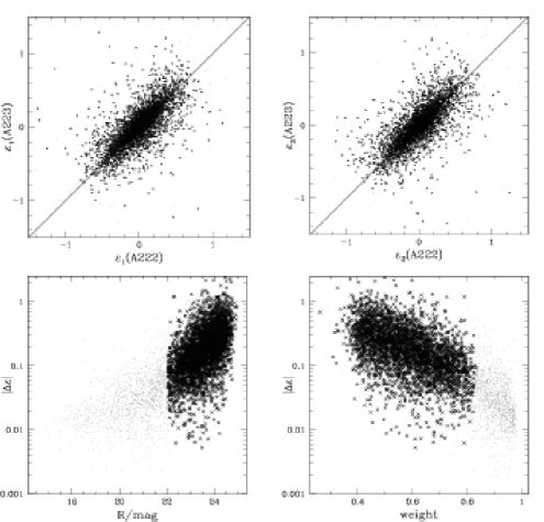
Figure 1: Reliability tests of the shear estimates of objects observed in the overlapping region of the two $R$-band pointings. All objects with shear estimates are plotted as light dots, objects surviving our various selection criteria, detailed in the text, are plotted as crosses. Top left: Scatter plot of the $\varepsilon_{1}$ component estimates from the exposures centered on A 222 versus the one centered on A 223. The diagonal line is not a fit but only represents the ideal relation. Although we delete objects with corrected ellipticity $|\varepsilon|>0.8$ from our final lensing catalog, some objects with $|\varepsilon|>0.8$ are marked with crosses in this plot. This is because the mean ellipticity of their two measurements, which we employ in our selection and lensing analysis is below the chosen cut-off level. These objects are strongly down-weighted and their exclusion would not lead to significant differences in the lensing analysis. Top right: Same for the $\varepsilon_{2}$ component. Bottom left: Dependence of the absolute value of differences of the shear estimators $|\Delta\varepsilon|$ on the apparent magnitude of the object. As expected, fainter objects have less reliable shear estimates. Bottom right: This panels shows the correlation between $|\Delta\varepsilon|$ and the weighting scheme we employed. Objects with higher weights have more reliable shear estimates.

The large overlap between the two $R$-band images allows us to test the reliability of the shear estimates and the validity of the weighting scheme we will employ in the lensing analysis. We perform these tests separately for the set of all objects found in the unmasked part of the overlap region, and the set of objects left after performing the various cuts described in the previous paragraph. The top panels of Fig. 1 show a comparison of the shear estimates of objects observed in the overlap region of the two $R$-band pointings. Overall, the two independent shear estimates agree but show a broad scatter around the ideal relation. For the set of all galaxies, we find that the mean of the differences between the two measurements is $-0.01$ for the $\varepsilon_{1}$ component and $0.00$ for the $\varepsilon_{2}$ component. The standard deviation is $0.20$ in each component. Erben et al. (2003) found an $rms$ scatter of $0.16$ between two different lensing analyses of their data. Our value seems to indicate that the additional scatter introduced by the independent observations is small compared to the uncertainties intrinsic to the shear estimation procedure. The bottom left panel of Fig. 1 shows the dependence of the absolute values of differences of the shear estimators $|\Delta\varepsilon|$ on the apparent $R$-band magnitude. As one expects, the reliability of the shear estimates drops dramatically for fainter objects. Because these are the objects we keep in our lensing catalog the $rms$ scatter between the two shear estimates increases to $0.25$ per component for the galaxies kept in our lensing catalog. The mean for the set of galaxies in our lensing catalog stays almost unchanged at $0.01$ in both components, showing that, while the shear estimates become noisier, no systematic differences between both images are present.

In the lensing reconstruction and the aperture mass maps (Schneider 1996) we will assign a weight to each shear estimator. The weight is computed by

$$w=\left(\sigma_{\varepsilon_{\mathrm{2D}}}^{2}+\sigma_{\mathrm{g}}^{2}\right)^{-1}\;,$$ (1)

where $\sigma_{\varepsilon_{\mathrm{2D}}}$ is the intrinsic 2-d ellipticity dispersion and $\sigma_{\mathrm{g}}$ is the error estimate of the initial ellipticity measurement of the galaxy. We set $\sigma_{\varepsilon_{\mathrm{2D}}}=0.38$ which is typically found in ground-based weak lensing observations (T. Erben, private communication; e.g. Clowe & Schneider (2001) who find a value of $\sigma_{\varepsilon_{\mathrm{2D}}}=0.42$). $\sigma_{\mathrm{g}}$ is computed from the uncertainty of the measurement of the quadrupole moment of the galaxy in the image. While both quantities are not independent – $\sigma_{\varepsilon_{\mathrm{2D}}}$ is of course increased by higher errors in the initial ellipticity measurement – their relation is very complex and not readily quantifiable in the KSB algorithm. As a consequence, galaxies with low $\sigma_{\mathrm{g}}$ probably receive less weight than they should in an ideal weighting scheme. The large overlap and the high number of objects detected in both frames would enable us to study the shear estimation procedure in more detail and probably find a better weighting scheme than the one used in this work. This is, however, beyond the scope of this paper.

The bottom right panel of Fig. 1 shows the correlation between our weights (normalized to be $\leq 1$) and $|\Delta\varepsilon|$. This verifies that galaxies with more reliable shear estimates have a higher weight in the generation of the lensing maps, although the large variations in $|\Delta\varepsilon|$ only correspond to small relative changes in the weight $w$. The shear estimates with the highest weight, not part of our lensing catalog, are those which we reject as probable foreground objects because they are too bright.

3.2 Weak lensing reconstruction

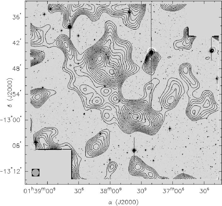
Figure 2: Weak lensing surface mass density contours overlaid on the $R$-band mosaic observed with the Wide-Field imager at the ESO/MPG-2.2m telescope. The shear field was smoothed with a $\sigma=1\aas@@fstack{\prime}{75}$ Gaussian, corresponding to the diameter of the circle at the lower left corner. Each contour represents an increase in $\kappa$ of 0.005 ($\sim 1.6\times 10^{13}\leavevmode\nobreak\ h_{70}\leavevmode\nobreak\ M_{\sun}$ Mpc^-2, assuming $\overline{z}_{\mathrm{FBG}}=1$) above the mean $\kappa$ at the edge of the field.

Based on the lensing catalog described in the previous section, the weak lensing reconstruction in Fig. 2 was performed using the Seitz & Schneider (2001) algorithm adapted to the field geometry with a $\sigma=1\aas@@fstack{\prime}{75}$ smoothing scale on a $214\times 200$ points grid.

Both clusters are well detected in the reconstruction, the two components of A 223 are clearly visible, and the elliptical appearance of A 222 is present in the surface-mass density map. The strong mass peak West of A 223 is most likely associated with the reflection ring around the bright $V=7.98$ mag star at that position. Although the prominent reflection ring was masked, diffuse stray light and other reflection features are visible, extending beyond the masked region, well into A 223, probably being the cause of this mass peak.

The peak positions in the weak lensing reconstruction are off-set from the brightest galaxy in A 222 and the two sub-clumps of A 223. The centroid of the mass of A 222 is $57\arcsec$ South-East of the brightest cluster galaxy (BCG); the mass centroids of A 223-N and A 223-S are $86\arcsec$ and $37\arcsec$ away from the BCGs of the respective sub-clumps.

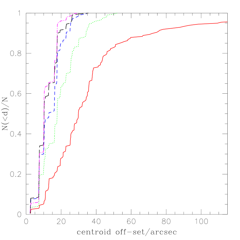
Figure 3: Cumulative fraction of off-set of the reconstructed centroids from the real centroid. The curves display the probability of finding a reconstructed centroid of an SIS with a velocity dispersion of 550 km s^-1(continuous), 700 km s^-1(dotted), 850 km s^-1(short dashed), 1000 km s^-1(long dashed), and 1150 km s^-1(dashed-dotted) from the real centroid position. The SIS was put at a redshift of $z=0.21$; the number density of the input catalog was 15 arcmin^-2.

To estimate the significance of these off-sets we performed lensing simulations with singular isothermal sphere (SIS) models of various velocity dispersions. The SIS models were put at the cluster redshift of $z=0.21$; catalogs with a random distribution of background galaxies with a number density of 15 arcmin^-2, and 1-d ellipticity dispersion of $\sigma_{\varepsilon_{\mathrm{1D}}}=0.27$ were created for 200 realizations. The shear of the SIS models was applied to the galaxy ellipticity of the catalog. Weak lensing reconstructions based on these catalogs were performed with the smoothing scale set $\sigma=1\aas@@fstack{\prime}{75}$ to match the smoothing of our real data. Due to the lower SNR for the 550 km s^-1SIS, the simulations yielded only 198 reliable centroid positions, while the centroid positions of the more massive SIS could be reliably determined in all 200 realizations. Fig. 3 shows the cumulative fraction of reconstructed peaks found within a given distance from the true centroid position.

These simulations show that the observed off-set of A 223-S is compatible with the statistical noise properties of the reconstruction. The off-set of A 222, using the the velocity determination of the SIS models fitted below, is significant at the 2-3$\sigma$ level. The off-set of A 223-N cannot be explained with the statistical noise of the reconstruction alone. It is, however, likely that the observed significant off-sets are not real but linked to the influence of the bright star and its reflection rings West of A 223. Although objects coinciding with this reflection ring were excluded from the catalog, the presence of a strong mass peak on the position of the bright reflection ring is a clear indication that the shear estimates are affected by the weaker reflection features which are too numerous and large to be masked. It is difficult to guess how these reflections could contribute to the observed peak shifts. We found that varying the size of the masked region did affect the strength of the peak on the reflection ring but left the off-sets of the cluster peaks essentially unchanged. Still, it is noteworthy that the mass peaks are shifted preferentially away from the star.

To avoid the mass-sheet degeneracy we estimate the cluster masses from fits of parameterized models to the shear catalog. The fits were performed minimizing the negative shear log-likelihood function (Schneider et al. 2000)

$$l_{\gamma}=-\sum_{i=1}^{N_{\gamma}}\ln p_{\varepsilon}(\varepsilon_{i}|g(\@vec{\theta}_{i}))\;$$ (2)

over the $N_{\gamma}$ galaxy images to obtain the parameter set most consistent with the probability distribution $p_{\varepsilon}(\varepsilon_{i}|g(\@vec{\theta}_{i}))$ of lensed galaxy ellipticities. See Schneider et al. (2000) for a detailed discussion of this maximum likelihood method for parameterized models. We fitted more than one mass profile simultaneously. Compared to a single model fit, this reduces the influence of the other cluster on the fitting procedure and result. Galaxies within distances $\theta<\theta_{\mathrm{min}}=3\arcmin$ from the centers of the models were ignored when fitting SIS models. Assuming a typical SIS this corresponds to roughly 10 Einstein radii and is enough to assume that all galaxies used in the fitting procedure are in the weak lensing regime. Ignoring galaxies close to the cluster centers also reduces the contamination with faint cluster galaxies. As a first approach we fit two SIS, one centered on the BCG of A 222, the other centered on the line connecting the BCGs of the two sub-clumps of A 223. The best-fit models in this case have velocity dispersions of $716^{+67}_{-74}$ km s^-1and $804^{+59}_{-64}$ km s^-1, respectively. This is considerably lower than the spectroscopic velocity dispersions of D02 of $1014^{+90}_{-71}$ km s^-1for A 222 and $1032^{+99}_{-76}$ km s^-1for A 223. It is also lower than the velocity dispersions derived from X-ray luminosities (David et al. 1999) and the $L_{\mathrm{X}}-\sigma$ relation of Wu et al. (1999), which are $845-887$ km s^-1and $828-871$ km s^-1, respectively (D02), but the value for A 223 is consistent within the error bars. The error bars of the individual velocity dispersion were computed from $2\Delta l$, where the velocity dispersion of one component was kept fixed at its best-fit value to give the errors estimate for the other component. The two component fit has a significance of $7.9\sigma$ over a model without mass. Joint confidence contours are displayed in Fig. 4.

Figure 4: Combined confidence contours for the SIS velocity dispersion of A 222 and A 223. The contour lines are drawn for $2\Delta l=\left\{2.3,4.61,6.17,9.21,11.8,18.4\right\}$, corresponding to the 63.8%, 90%, 95.4%, 99%, 99.73%, and 99.99% confidence levels, respectively, under the assumption that the statistics is approximately Gaussian.

A three component model with an SIS centered on each BCG has a lower significance over a zero mass model than the two SIS model and does not fit the data better.

Because both clusters are elliptical and the masses determined from SIS fits differ strongly from those derived by D02, one might assume that fitting elliptical mass profiles yields a more accurate estimate of the cluster mass. To test this, we fitted singular isothermal ellipse models to the clusters. It turned out that the 6 parameter fit necessary to model both cluster simultaneously was very poorly constrained and the fit procedure was not able to reproduce the orientation of the clusters. Results strongly depended on the initial values chosen for the minimization routines.

Figure 5: Confidence contours for the best-fit NFW parameters for A 222 (left panel) and A 223 (right panel). The contours are drawn at the same levels as in Fig. 4.

The best-fit NFW models have $r_{200}=1276^{+102}_{-121}h_{70}^{-1}$ kpc, $c=3.4$ and $r_{200}=1546^{+145}_{-151}h_{70}^{-1}$ kpc, $c=1.2$ for A 222 and A 223, respectively, excluding shear information at distances $\theta<1\aas@@fstack{\prime}{5}$ from the cluster centers. The NFW models have a significance of $5.2\sigma$ over a model with no mass. Fig. 5 shows confidence contours for the NFW fits to the individual clusters, computed from $2\Delta l$, while keeping the best-fit parameters for the other cluster fixed. We summarize the derived cluster properties in Tab. 1.

Table 1: Summary of the cluster properties derived from spectroscopy, X-ray, and weak lensing observations.

	A 222	A223
$\sigma_{\mathrm{vir}}$/(km s-1)	$1014^{+90}_{-71}$	$1032^{+99}_{-76}$
$\sigma(L_{\mathrm{X}})$/(km s-1)	845–887	828–871
$\sigma_{\mathrm{SIS}}$/(km s-1)	$716^{+67}_{-74}$	$804^{+59}_{-64}$
$r_{200}$/(kpc $h_{70}^{-1}$)	$1276^{+102}_{-121}$	$1546^{+145}_{-151}$

As we see from the left panel in Fig. 5, it can be difficult to obtain reliable concentration parameters from weak lensing data. The reason is that the shear signal is mostly governed by the total mass inside a radius around the mass center. Only in the cluster center the shear profile carries significant information about the concentration parameter. For example if we set $\theta_{\mathrm{min}}=3\arcmin$ – like we did for fitting SIS models – in the minimization procedure, $M_{200}$ remains essentially unchanged while the concentration factor can increase dramatically. The best fit parameters for A 222 in this case are $r_{200}=1238h_{70}^{-1}$ kpc, $c=7.8$. If we choose the radius $\theta_{\mathrm{min}}$ inside which we ignore galaxies too big, typical values for the scale radius $r_{\mathrm{s}}=r_{200}/c$ are contained within this radius. $c$ is then essentially unconstrained, i.e. the minimization procedure cannot anymore distinguish between a normal cluster profile and a point mass of essentially the same mass.

The situation is different for A 223. The two sub-clumps are separated by $\sim 4\arcmin$. This means that even ignoring shear information within the larger $\theta_{\mathrm{min}}=3\arcmin$ radius, the outer slopes of the sub-clumps are outside $\theta_{\mathrm{min}}$ and the determination of the concentration parameter gives a tight upper bound and does not change as dramatically when the minimization is performed only with galaxies further away from the cluster center as is the case in A 222. Because the shear outside $\theta_{\mathrm{min}}$ is effectively that of an averaged mass profile inside $\theta_{\mathrm{min}}$ the measured concentration parameter is very low.

The projected cluster separation is marginally smaller than the sum of the virial radii ($r_{\mathrm{vir}}\sim r_{200}$) derived from the shear analysis; $r_{200}(\mathrm{A\leavevmode\nobreak\ 222})+r_{200}(\mathrm{A\leavevmode\nobreak\ 223})=2822^{+177}_{-193}h_{70}^{-1}\,\mathrm{kpc}$. We have to emphasize that this is only the projected separation. D02 found redshifts of $z=0.2126\pm 0.0008$ for A 222 and $z=0.2079\pm 0.0008$ for A 223. Assuming that both clusters participate in the Hubble flow with no peculiar velocity, this redshift difference of $\Delta z=0.005\pm 0.001$ translates to a physical separation along the line of sight of $(15\pm 3)h_{70}^{-1}$ Mpc. Presumably, part of the observed redshift difference is due to peculiar velocities. In any case, it is more likely that the two clusters are physically separated and the virial radii do not overlap.

3.3 A possible dark matter filament

Also visible in the reconstruction is a bridge in the surface mass density extending between A 222 and A 223. Although the signal of this possible filamentary connection between the clusters is very low, the feature is quite robust when the selection criteria of the catalog are varied and it never disappears. Variations on the selection criteria of the catalog let the filament shift a few arcminutes in the East-West direction. The filament strength also changes but on closer inspection this can be attributed almost entirely to variations in the mass-sheet degeneracy, which is fixed by setting the mean $\kappa$ at the edge of the field to zero. Although the field is big enough to assume that the clusters have no considerable contribution to the surface mass density at the edge of the field, this is a region where the $\kappa$-map is dominated by noise. Small changes in the selection criteria can change the value of the mass-sheet degeneracy by as much as $\kappa_{0}=0.02$. This illustrates that a surface mass density reconstruction is not suitable to assess the significance of structures as weak as filaments expected from $N$-body simulations. We try to develop methods to quantify the significance of this signal in section 5.

3.4 Other mass peaks

In addition to the cluster peaks several other structures are seen in the reconstruction in Fig. 2. Using the aperture mass statistics (Schneider 1996) with a $6\aas@@fstack{\prime}{4}$ filter scale we find that the peak $\sim 13\arcmin$ SE of A 222 has a SNR of $3.5$. This peak corresponds to a visually identified overdensity of galaxies.

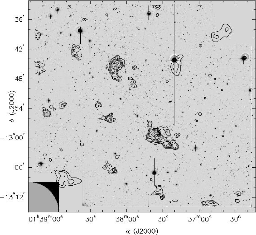
Figure 6: Shown above are SNR contours of the aperture mass statistics with a $6\aas@@fstack{\prime}1$ filter radius overlaid on the WFI $R$-band image. The lowest contour is at $2.0$, higher contours rise in steps $0.5$. The mass peak $\sim 13\arcmin$ SE of A 222 has a peak SNR of $3.5$. The circle segment in the lower left corner has the same radius as the filter function.

Figure 7: Color magnitude diagram of objects around the mass peak SE of A 222. A possible red-cluster sequence can be seen around $V-R\approx 1.1$.

Fig. 7 shows a $V-R$ vs. $R$ color-magnitude diagram of all galaxies in a box with $170\arcmin$ side length around the brightest galaxy in this overdensity. A possible red-cluster sequence (RCS) can be seen centered around $V-R=1.1$, which would put this mass concentration at a redshift of $z\sim 0.4$. However, the locus of the RCS is so poorly defined that this estimate has a considerable uncertainty. Assuming this redshift, the best-fit SIS model has a velocity dispersion of $728^{+101}_{-120}$km s^-1and a significance of $3.2\sigma$ over a model without mass. The best-fit NFW model has $r_{200}=1322h_{70}^{-1}$ kpc and $c=3.3$ and a significance of $2.8\sigma$ over a model with $r_{200}=0$, determined from $\delta\chi^{2}$.

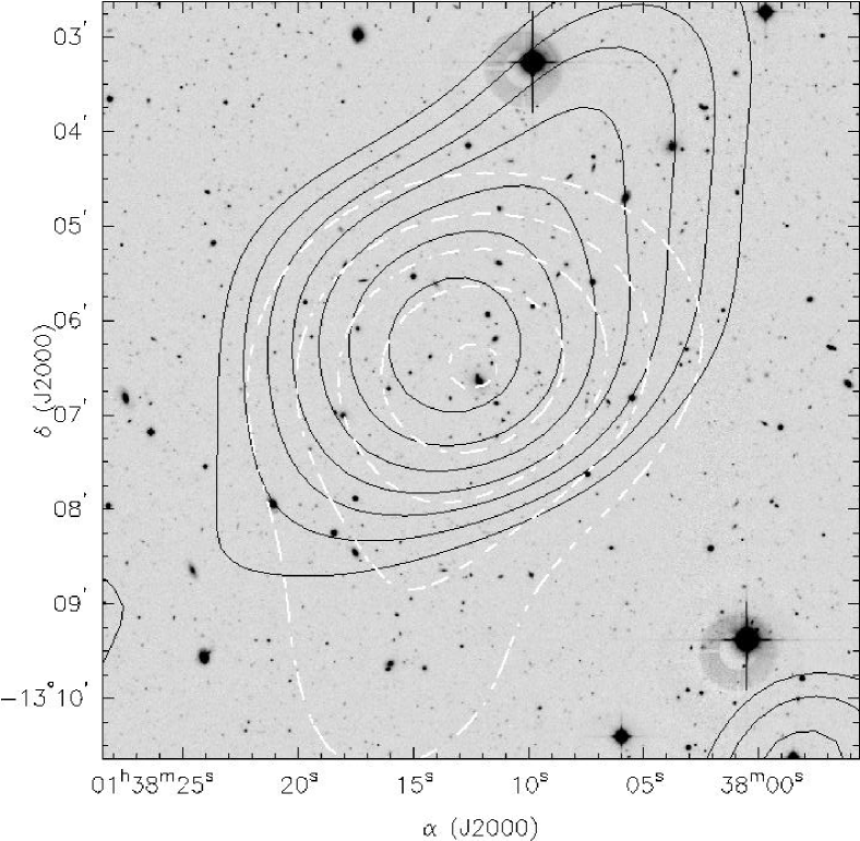
Figure 8: Mass and light contours in the peak SE of A 222. Black solid lines are contours of the mass reconstruction in Fig. 2, white dashed lines denote the luminosity density of galaxies with $1.0<V-R<1.2$.

Fig. 8 shows a comparison of surface mass and luminosity density for this peak. Galaxies with $1.0<V-R<1.2$ were selected to match the tentative RCS from Fig. 7. The figure shows excellent agreement between the mass and light contours, unambiguously confirming that this is a weak lensing detection of a previously unknown cluster. The off-set between the mass centroid and the BCG, which is located at $\alpha$=01:38:12.1, $\delta$=$-$13:06:38.2, is $27\arcsec$ and not significant for an SIS with a velocity dispersion of $\sim 730$ km s^-1at a redshift of $z\sim 0.4$.

The mass concentration in the Western part of the possible filament reaches a peak SNR of $3.6$ at a filter scale of $3\aas@@fstack{\prime}{2}$. We do not find an overdensity in the number or luminosity density of galaxies at this position. None of the other mass peaks seen in the reconstruction, with exception of the one on the reflection ring, is significant in filter scales $>2\aas@@fstack{\prime}{4}$.

4 Comparison of mass and light in A 222/223

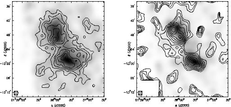
Figure 9: Smoothed distribution of the number density (left panel) and the luminosity density (right panel). The smoothing was done with a $\sigma=1\aas@@fstack{\prime}{75}$ Gaussian to match the smoothing of the weak lensing reconstruction. The diameter of the circles at the lower left corners corresponds to the FWHM of the Gaussian. The contour lines in the left panel are significance contours starting at $5\sigma$ and rising in steps of $1\sigma$, the contour lines in the right panel are the surface mass density contours of the reconstruction.

Fig. 9 shows the number density and luminosity distribution in the A 222/223 system. The left panel shows the number density distribution of the color-selected ($0.78<V-R<0.98$) early-type galaxies. The contours lines indicate the SNR determined from bootstrap resampling the selected galaxies. It is evident that a highly significant overdensity of early-type galaxies exists in the intercluster region. The right panel shows a comparison between luminosity (background gray-scale image) and surface mass density. In general, there is good agreement between the two. We again note the off-sets of the mass centroids from the light distribution, which we attribute to the systematics induced by the reflection ring. The elongation of A 222 is nicely reproduced in the reconstruction. A 222 is the dominant cluster in the luminosity density map, while in the mass reconstruction A 223 appears to be more massive. We note, however, that many of the bright E/S0 galaxies in A 223 escape our color selection because they are bluer than expected for early-type galaxies at this redshift. This indicates a high amount of merger activity in this irregular system and most likely still collapsing system. As we fixed the colors such that the RCS matches the expected colors of early-type galaxies at the cluster redshift, this clearly shows that the bright central galaxies in A 223 are bluer than expected.

The overdensity in number and luminosity density is not aligned with the dark matter filament candidate. We should, however, not forget that the position of the filamentary structure is somewhat variable with varying cuts to the lensing catalog. If the reflection features West of A 223 are indeed responsible for shifting the centroid positions of the massive clusters, their effect may be even stronger on such weak features as the mass bridge seen in the reconstruction.

We estimate the cluster luminosities by measuring the $R$-band luminosity density of all galaxies within $r_{200}$ – as determined from the lens models in Sect. 3.2 – in excess of the luminosity density in a circle with $5\arcmin$ radius centered on (01:36:45.8, $-$13:07:25), which is an empty region in the SW of our field. A 222 has a luminosity $L_{R,\,r_{200}}=(2.7\pm 0.4)\times 10^{12}\,h^{-2}\,L_{\sun}$ and A 223 has a luminosity of $L_{R,\,r_{200}}=(5.6\pm 0.8)\times 10^{12}\,h^{-2}\,L_{\sun}$. Using the mass determined from the NFW profiles, this implies rather low $M/L$ ratios; $M/L_{R}=111^{+31}_{-34}\,h_{70}\,M_{\sun}/L_{\sun}$ for A 222 and $M/L_{R}=95^{+30}_{-31}\,h_{70}\,M_{\sun}/L_{\sun}$ for A 223. The mass-to-light ratios increase to $M/L_{R}=178^{+45}_{-49}\,h_{70}\,M_{\sun}/L_{\sun}$ and $M/L_{R}=131^{+30}_{-31}\,h_{70}\,M_{\sun}/L_{\sun}$ for A 222 and A 223, respectively, if the mass estimates from the SIS models within $r_{200}$ are used.

The X-ray satellite ROSAT observed the pair of galaxy clusters on 16. January 1992 using the position sensitive proportional counter (PSPC). We extracted these data from the public ROSAT archive in Munich and analyzed the total integration time of 6780 seconds using the EXSAS software (Zimmermann et al. 1998). To avoid any confusion with diffuse soft X-ray emission and associated photoelectric absorption towards the area of interest, we focused our scientific interest on the upper energy limit of the PSPC detector. Using the pulse height invariant channels 51 – 201 (corresponding to $0.5\,\mathrm{keV}\leq\,E\,\leq\,2.1\,\mathrm{keV}$) we calculated the photon image and the corresponding “exposure-map” according to the standard data reduction. We performed a “local” and a “map” source detection which in total yielded 42 X-ray sources above a significance threshold of ten.

By visual inspection, we selected some X-ray sources located close to the diffuse X-ray emission of the intra-cluster gas and subtracted their contribution using the EXSAS task create/bg_image. This task subtracts the X-ray photons of the point sources and approximates the background intensities via a bi-cubic spline interpolation. Finally the X-ray data were smoothed to an angular resolution of $1\aas@@fstack{\prime}{75}$ using a Gaussian smoothing kernel.

Contours for this final image are shown in Fig. 10. Detected X-ray sources kept in the final image are marked with circles; the subtracted unresolved sources are denoted by stars. The lowest contour line is at the $3\sigma$ level. Higher contours increase in steps of $2\sigma$. Both cluster are very well visible. As already noted by Wang & Ulmer (1997), A 223-S is by far the dominant sub-clump in A 223 in X-ray.

A bridge in X-ray emission connecting both clusters is seen at the $5\sigma$ level in this image. This possible filament is aligned with the overdensity of the number density of color selected galaxies but not with the filament candidate seen in the weak lensing reconstruction.

The Eastern spur in the X-ray emission of A 223 is caused by a point source whose removal would cut significantly into the cluster signal. We therefore decided to keep this source. Removing it does not influence the signal in the intercluster region. The Northern extension of A 223 in the $\kappa$ map is blinded by the support structure of the PSPC window in the X-ray exposure.

5 Quantifying filaments

In Sect. 3 we found a possible dark matter filament extending between the clusters A 222 and A 223 but its reality and significance are not immediately obvious. In this section we try to develop a method to quantify the significance of weak lensing filament candidate detections.

To quantify the presence of a filament and the significance of its detection, two problems must be solved. First the fundamental question “What is a filament?” must be answered. How, for instance, is it possible to discriminate between overlapping halos of two galaxy clusters and a filament between two clusters? While in the case of large separations this may be easy to answer intuitively, it becomes considerably more difficult if the cluster separation is comparable to the size of the clusters themselves (see e.g. the left panel of Fig. 9).

Figure 10: To the left is an overlay of X-ray contours (white lines) over the WFI images of our field. The contour lines start at $3\sigma$ and increase in steps of $2\sigma$. All detected X-ray sources are marked; circles correspond to sources kept, while the point sources excised from the image are marked with stars. The X-ray image was smoothed with a $\sigma=1\aas@@fstack{\prime}{75}$ Gaussian, corresponding to the diameter of the circle at the lower left corner. The black contours in the background are the significance contours of the number density from the left panel of Fig. 9.

The second problem – quantifying the significance of a filament detection – is rooted in the weak lensing technique. To avoid infinite noise in the reconstruction, the shear field must be smoothed (Kaiser & Squires 1993). This leads to a strong spatial correlation of the $rms$ error in the reconstructed $\kappa$ map, making it difficult to interpret the error bars at any given point. Randomizing the orientation of the faint background galaxies while keeping their ellipticity moduli constant and performing a reconstruction on the randomized catalog allows one to assess the overall noise level as $\left<\kappa^{2}_{\mathrm{rand}}\right>$. While this can be used to determine the noise level, the mass-sheet degeneracy (Schneider & Seitz 1995) allows us to arbitrarily scale the signal.

Statistics like the aperture mass (Schneider 1996) and aperture multipole moments (Schneider & Bartelmann 1997) allow the calculation of signal-to-noise rations for limited spatial regions and are thus well suited to quantify the presence of a structure in that region. Hence, to quantify the presence of a structure between two galaxy clusters, the aperture has to be chosen such that it avoids the clusters and is limited to the filament candidate. This is of course closely related to the first problem. We will discuss in the following sections how aperture statistics could be used to determine the SNR of a possible dark matter filament.

We use $N$-body simulations of close pairs of galaxy clusters to find solutions to these problems.

5.1 $N$-body simulations

Since we are interested in developing a method for a very particular mass configuration, it is desirable to work with $N$-body simulations that could mimic as closely as possible the A 222 and A 223 cluster system. This goal can be achieved by performing constrained $N$-body simulations.

Constrained realizations were first explored by Bertschinger (1987), and later presented in an elegant and simple formalism by Hoffman & Ribak (1991). Here we follow the approach of van de Weygaert & Bertschinger (1996) of the so-called Hoffman-Ribak algorithm for constrained field realizations of Gaussian fields. With this approach, the constructed field obeys the imposed constraints and replaces the unconstrained field.

The cluster-bridge-cluster system intended to simulate resembles a quadrupolar matter distribution. It is therefore expected that primeval tidal shear plays an important role in shaping such matter configuration (see van de Weygaert 2002 for a review), which must have been induced by tiny matter density fluctuations in the primordial universe.

In moulding the observational data we have considered each one of the observational aspects and cosmological characteristics of the system. We have put constraints onto the initial constrained field to create the two clusters and the bridge in the following way:

Two initial cluster seeds were sowed at the center of the simulation box, separated by a distance $d$. We imposed constraints over the clusters themselves like peak height (1 constraint), shape (3 constraints), orientation (3 constraints), peculiar velocity (3 constraints) and tidal shear (5 constraints).

We have performed a set of 10 realizations in a periodic $50h^{-1}_{70}$ Mpc box, with different combinations of the mentioned 18 constraints. In all simulations we set $h_{70}=0.7$, i.e. $H_{0}=50$ km s^-1. All constraints were imposed over a cubic grid of $64$ grid-cells per dimension. In all 10 realizations, all constraints were defined on a Gaussian scale $r_{g}$ of $4\,h_{70}$ Mpc for both clusters. Because we are dealing with rich clusters, we have imposed a peak height $f_{G}=3\sigma_{0}$, where $\sigma_{0}$ is the variance of the smoothed density field ($\sigma_{0}(r_{g})=\langle f_{g}f_{g}\rangle^{1/2}$). The other constraints considered were: oblate clusters with axis ratios $\lambda_{2}/\lambda_{1}=0.9$ and $\lambda_{3}/\lambda_{1}=0.8$ and both major axes aligned with each other. We have imposed a “weak” primordial tidal field in order to produce a realistic field around the clusters. The stretching mode of the tidal field was aligned along the same direction given by the major cluster axes. The compressional mode was set perpendicular to the bridge axis. This combination of constraints proved to be the most successful one in reproducing (in the linear regime) the configuration presented by the two Abell clusters.

The initial particle displacements and peculiar velocities were assigned according to the Zel’dovich (1970) approximation from the constrained initial Gaussian density field. The evolution of the linear constrained density field into the non-linear regime was performed by means of a standard P³M code (Bertschinger & Gelb 1991). The number of grid-cells used to evaluate the particle-mesh force was $128^{3}$, with a particle mass resolution of $3.3\times 10^{10}M_{\sun}$. We selected 15 time outputs in order to follow the simulation through the non-linear regime, with a time output at redshift $z=0.21$, to match the observed cluster redshift. Fig. 11 shows the most successful cluster-bridge-cluster configuration.

To estimate the underlying smooth mass distribution from the result of the simulations, the particle distribution was smoothed using the adaptive kernel density estimate described by Pisani (1996, 1993). A comparison of the simulated and smoothed mass distribution can be found in Figs. 11 and 12.

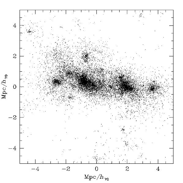
Figure 11: Zoom in on the central $10\times 10$ Mpc²/$h_{70}^{2}$ of an $N$-body simulation. Displayed is the projection of a slice of 2.5 Mpc/$h_{70}$ thickness.

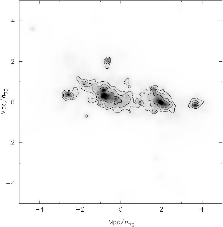
Figure 12: Smooth density distribution of the data in the left panel from the adaptive kernel density estimate. The contours are at $\kappa=\{0.03,0.05,0.1,0.5\}$.

The surface mass density of all simulations was linearly scaled such that $\kappa_{\mathrm{max}}\simeq 1$.

We have also computed the density field by means of the Delaunay Tessellation Field Estimator (Schaap & van de Weygaert 2000), which in principle offers higher spatial resolution at both, dense and underdense regions in comparison with other fixed-grid or adaptive kernels density reconstruction procedures.

The reconstructed DTFE surface mass density maps of the cluster-bridge-cluster system agree with those from the adaptive kernel since in high-density regions, both methods give similar density estimates (Pelupessy et al. 2003).

The lensing properties of the smoothed mass distribution were computed on a $2048\times 2048$ points grid using the kappa2stuff program from Nick Kaiser’s IMCAT software package. kappa2stuff solves the Poisson equation

$$\nabla^{2}\psi(\@vec{\theta})=2\kappa(\@vec{\theta})$$ (3)

in Fourier space on the grid by means of a Fast Fourier Transformation (FFT) and returns – among other quantities – the complex shear $\gamma(\@vec{\theta})$ and the magnification $\mu(\@vec{\theta})$.

For the lensing simulation, catalogs of background galaxies were produced. Galaxies were randomly placed within a predefined area until the specified number density was reached. To each galaxy an intrinsic ellipticity was assigned from two Gaussian random deviates. Unless noted otherwise all simulations have 30 galaxies/arcmin² and a one-dimensional ellipticity dispersion of $\sigma_{\varepsilon_{\mathrm{1D}}}=0.2$.

To test the validity of our lensing simulation we performed a mass reconstruction of the simulation in Fig. 12 using the algorithm of Seitz & Schneider (2001). The smoothing scale in this reconstruction was set to $1\aas@@fstack{\prime}{3}$. The result is shown in Fig. 13. We see that the reconstruction successfully recovers the main properties of the density distribution; both clusters are clearly detected, their ellipticity and orientation agrees with that of the smoothed density field. A “filament” resembling that in Fig. 12 is also seen. We now have to find a way to determine the significance of its detection.

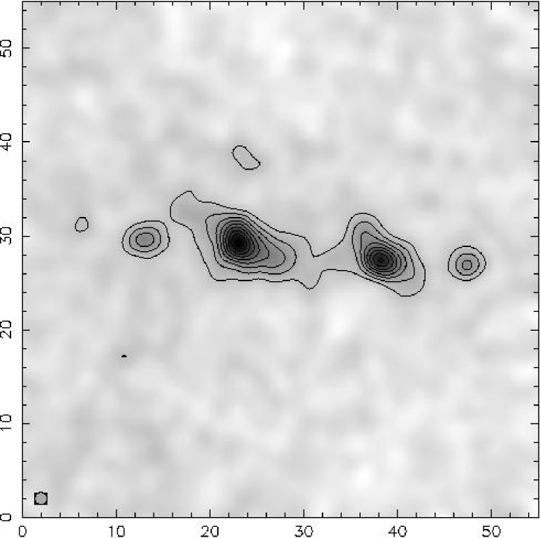
Figure 13: Reconstruction of the mass distribution in Fig. 12 on a $206\times 206$ points grid. The scale of the axes is given in arcminutes. The contours mark an increase of $\kappa$ in steps of 0.025 above the mean of the edge of the field. The diameter of the circle in the lower left is equal to the FWHM of the Gaussian smoothing of the shear field.

5.2 Fitting elliptical profiles to galaxy clusters

In a first attempt to quantify filaments, we try to fit the galaxy clusters by elliptical mass profiles. We then define the filament as the part of the mass distribution which is in excess of the mass fitted by the ellipses.

The profile we used is the non-singular isothermal ellipse of Keeton & Kochanek (1998). This profile has four parameters per cluster that need to be fitted:

• The axis ratio

• The core radius

• The Einstein radius of the corresponding singular isothermal sphere

• The orientation of the ellipse

The central position was fixed and taken to be the peak position of the mass reconstruction. As in Sect. 3.2 we use the shear-log-likelihood function to fit more than one mass profile simultaneously.

Various methods for multidimensional minimization are available. All programs used for fitting either used the Downhill Simplex or Powell’s Direction Set algorithms discussed in detail in Press et al. (1992). We could not find any systematic differences between the results of the two methods. In general, their results agreed quite well if the same initial values were used.

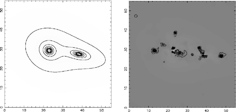
Figure 14: Left: Fit of two NIE profiles to the simulation in Fig. 12. The contour lines increase from $\kappa=0.025$ to $\kappa=0.25$ in steps of 0.025. Right: Difference image of Fig. 12 and the left panel. The contours are at the same level as in the left panel. The filament was completely subtracted. The surface mass density in the intercluster region is mostly negative.

Fig. 14 shows a fit of two non-singular isothermal ellipse (NIE) profiles to the simulation in Fig. 12. We see that the cluster are roughly fitted by the NIE profiles. Like in the case of fitting SIE models to A 222/223, the ellipticity of the original cluster is only poorly reproduced. Varying the initial values of the minimization procedure, gives comparable best-fit values for the Einstein and core radius. The axis ratio and orientation of the ellipse are so strongly affected by the choice of initial values, that they have a profound impact on the surface mass density in the intercluster region. Especially, the orientation is only poorly constrained. Generally, the fits overestimate the surface mass density in the intercluster region, fitting the “filament” completely away. The behavior of the fits to the simulated data confirms our experience with fitting SIE profiles in the A 222/223 system. Letting the slope of the density profile vary does not remedy the problem. The shear log-likelihood function is rather sensitive to the slope of the density profile, but the ellipticity of the clusters is still poorly constrained.

5.3 Using aperture multipole moments to quantify the presence of a filament

Aperture multipole moments (AMM) quantify the weighted surface mass density distribution in a circular aperture. If it is possible to find a characteristic mass distribution for filaments and express it in terms of multipole moments, AMM can be used to quantify the presence of a filament.

Figure 15: Simple toy model of two galaxy clusters connected by a filament. A quadrupole moment is present in the aperture centered on the filament.

Figure 16: Toy model of two galaxy clusters without a filament, illustrating why it is important to choose the correct size of the aperture.

Fig. 15 illustrates with the help of a simple toy model of two galaxy clusters connected by a filament why one expects to find a quadrupole moment in an aperture centered on the filament. Fig. 16 illustrates that it is crucial not to choose the aperture too large. If the aperture also covers the clusters, a quadrupole moment will be measured even if no filament is present.

We choose a weight function

$$U(\theta)=\begin{cases}1-\left(\frac{\theta}{\theta_{\mathrm{max}}}\right)^{2}&\theta\leq\theta_{\mathrm{max}}\leavevmode\nobreak\ ,\\ 0&\text{otherwise}\leavevmode\nobreak\ ,\end{cases}$$ (4)

to compute the aperture quadrupole moment as defined in Schneider & Bartelmann (1997, see also Appendix B). While this weight function is clearly not ideal as it does not closely follow the mass profiles of the simulated data, it is sufficient to identify all relevant features in quadrupole moment $|Q^{(2)}|$ maps. Fig. 17 shows such $|Q^{(2)}|$ maps for the simulation in Fig. 12. In the quadrupole maps $\theta_{\mathrm{max}}$ increases from 2′to 5′. The maps were computed on $55\times 55$ points grid, so that each grid point is $1\arcmin\times 1\arcmin$ big. Overlayed are the contours of the surface mass density of the reconstruction of Fig. 13.

One clearly sees that the quadrupole moment between the clusters increases as the size of the apertures increases. This is of course expected and due to the growing portion of the clusters in the aperture, so that their large surface mass density dominates the mass distribution. Fig. 17 also illustrates the problem of separating clusters from a filament. The virial radii of the clusters extend far beyond the mass contours of the clusters in most directions and thus beyond what can be detected with weak lensing. Due to the ellipticity of the clusters it is not obvious whether the projected mass extending out to the virial radius is part of the cluster or belongs to a filament. While we certainly can define that projected mass outside the virial radii belongs to a filament, the case is not clear for mass inside $r_{200}$. The surface mass density contours in Fig. 17 seem to suggest that a signature of a filament is present and observable with weak lensing inside the virial radius. Because weak lensing only has a chance to detect filaments in close pairs of clusters whose separation is comparable to the sum of their virial radii, understanding this signature is important.

In this context the two maps in the top panel which show the smallest overlap of the aperture with the virial radii are the most interesting. Noteworthy in Fig. 17 is also that the top panels show a quadrupole moment on a ring-like structure around each cluster center. This is indeed to be expected for all galaxy clusters because there is a non-vanishing quadrupole moment if the aperture is not centered on the cluster center, but somewhere on the slope of the mass distribution. This now raises the question how we should distinguish the quadrupole moment present around any cluster from that caused by a filamentary structure between the clusters.

To better understand the features visible in the $|Q^{(2)}|$ maps of the $N$-body simulations we qualitatively examine the structures of a quadrupole map for a system of two isolated clusters and two clusters connected by a filament using simple toy models. Fig. 18 shows noise-free quadrupole maps of two truncated NFW halos (Takada & Jain 2003) without (top panel) and with (bottom panel) a connecting filament for the same aperture sizes as in the top panel of Fig. 17. The halo centers and virial radii were chosen to match those in the $N$-body simulation. To describe the filament we choose a coordinate system such that the $x$-axis runs through the halo centers and has its origin at the center between the clusters separated by a distance $d$ and define the following function:

$$\kappa_{\mathrm{fil}}(x,y)=k_{0}\frac{\left(k_{1}x^{4}+k_{2}x^{2}\right)\left|\frac{d}{2}-x\right|}{\left(y/k_{3}\right)^{2}+1}H\left(\left|\frac{d}{2}-x\right|\right)\,$$ (5)

where $k_{1}<0$ and $k_{2}$ chosen such that the maxima of the fourth order polynomial coincide with the halo centers. $H(x)$ is the Heaviside step-function.

As in the $|Q^{(2)}|$ maps of the $N$-body simulations a quadrupole moment related to the slope of the clusters is visible. Already the smallest aperture (left panel) overlaps the truncated NFW halos and leads to a strong quadrupole moment in the intercluster region. This quadrupole moment is, however, much weaker than it is in the presence of a filament (bottom panel of Fig. 18). Additionally, the presence of a filament is indicated by a ring structure on which the quadrupole moment is lower. This structure becomes more prominent with increasing filter radius. All aperture statistics act as bandpass filters on structure comparable in size to the filter radius. As the ring has a radius of $\sim 7\arcmin$ it is better visible in the map generated from the larger filter. This structure is present only in the halo-filament-halo system and not in the halo-halo system, even for filter scales larger than those depicted in Fig. 18. This structure is also visible in the quadrupole maps of the $N$-body simulations. It is well visible in the top right panel of Fig. 17 and less well visible but still present in the top left panel of Fig. 17. Thus, the quadrupole maps clearly indicate that the measured quadrupoles on the filament are not caused by a situation without filament like that illustrated in Fig. 16. Unfortunately, this ring structure, like the filament itself, is a visual impression that does not lend itself easily to a quantitative assessment of the presence of a filament.

These toy models and the $N$-body simulation show that the aperture quadrupole statistics is indeed sensitive to filamentary structures. The quadrupole moment of a halo-filament-halo system exceeds that of a pure halo-halo system. As the measured quadrupole moment strongly depends on the size of the aperture, choosing the appropriate aperture is important. A decomposition of a halo-filament-halo system into halo and filament components could be provide an objective criterion for chosing the filter scale.

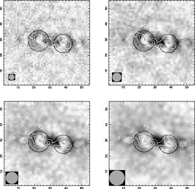
Figure 17: Quadrupole moment of the simulation in Fig. 12. Overlayed are the contours of the mass reconstruction in Fig. 13 and large circles with radius $r_{200}$ as determined from the 3-dimensional simulated data. $|Q^{(2)}|$ was computed in an aperture with radius $\theta_{\mathrm{max}}=2\arcmin$ (top left), $\theta_{\mathrm{max}}=3\arcmin$ (top right), $\theta_{\mathrm{max}}=4\arcmin$ (bottom left), $\theta_{\mathrm{max}}=5\arcmin$ (bottom right). The circles at the lower left corners have the same radii as the filter function in the respective panel. The cluster on the left has a mass of $M_{200}=2.0\times 10^{14}M_{\sun}$, the one on the right of $M_{200}=1.4\times 10^{14}M_{\sun}$.

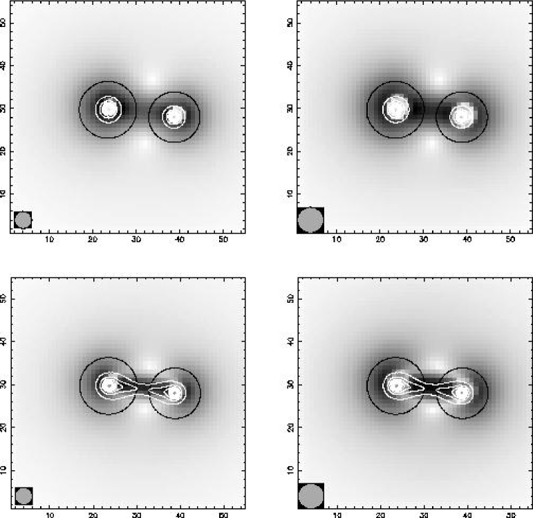
Figure 18: $|Q^{(2)}|$ maps of toy models of two clusters. Top panel: without a connecting filament. Bottom panel: with a filament running between both clusters. Quadrupole moments in the left panel were computed in a $2\arcmin$ aperture, in the right panel in a $3\arcmin$ aperture. The radii of the apertures correspond to the radii of the circles at the lower left corners of the respective panel. White contours are surface mass density; the black circles correspond the $r_{200}$ of the clusters.

While in the (failed) attempt to separate the clusters and the filament by fitting elliptical profiles to the clusters, the filament was naturally defined as the surface mass density excess above the clusters, there is no criterion in the AMM statistics that defines cluster and filament regions. We try to develop such a criterion in the following section.

5.4 Defining cluster and filament regions

Fig. 19 shows a simple one-dimensional toy model of the mass distribution of a cluster with a filamentary extension. The model consists of the following components: We assume a cluster with a King profile. This is the solid line in Fig. 19. In all simulations we see that the clusters are not spherical but triaxial with their major axes oriented approximately towards each other. We account for this in the model by stretching the right half of the King profile (long dashed line) by a factor $f$, which has to be determined, i.e. the original profile $\kappa_{\mathrm{King}}(\theta)$ is replaced with $\kappa_{\mathrm{stretch}}(\theta)\equiv\kappa_{\mathrm{King}}(f\theta),\,0<f\leq 1$, for positive values of $\theta$. We will call $f$ the “stretch factor”. The contribution of the filament (dotted line) $\kappa_{\mathrm{fil}}(\theta)$ is added to the stretched King profile. The result is the observed surface mass density profile on the right-hand side (short dashed) which can be described by

$$\kappa_{\mathrm{obs}}(\theta)=\kappa_{\mathrm{King}}(f\theta)+\kappa_{\mathrm{fil}}(\theta)\;.$$ (6)

Figure 19: Simple model of the surface mass density distribution of an elliptical cluster and a filamentary extension along the main axis of the system. The solid line is a symmetric King profile, the long dashed line is the same King profile stretched by a factor to introduce the ellipticity seen in simulation. The filament is modeled as a separate component (dotted line). The observed profile (short dashed line) is the sum of the filament and the stretched King profile. The axes are labeled in arbitrary units. The vertical lines exemplify typical values for $\theta_{\mathrm{fit}}$ and $\theta_{\mathrm{cut}}$; see text for details.

Since the mass profile of the filament alone is not accessible by observations, we have to determine a point on the observed mass profile $\kappa_{\mathrm{obs}}(\theta)$ that we treat as the “end” of the cluster and the “start” of the filament. We tried this using the following procedure: The unstretched King profile, observed on the left-hand side where $\theta<0$, is stretched by the factor $f$, to model the influence of tidal stretching. By this step we try to obtain the (unobservable) cluster profile $\kappa_{\mathrm{stretch}}(\theta)$ on the right side without the contribution of the filament.

This stretched profile is then compared to the observed profile $\kappa_{\mathrm{obs}}$ containing the contribution of the filament by computing the goodness of fit

$$\chi^{2}=\sum_{i=i_{0}}^{N}\left(\frac{\kappa_{\mathrm{stretch}}(\theta_{i})-\kappa_{\mathrm{obs}}(\theta_{i})}{\sigma_{i}}\right)^{2}\leavevmode\nobreak\ ,$$ (7)

at sample points $\theta_{i}$ in the reconstruction along the main axis of the system. Typically, the spacing of the sample points will be that of the grid on which the reconstruction was performed. Linear interpolation between grid points will be used if the sampling points do not exactly coincide with the grid points. $\sigma_{i}$ is the estimated error in $\kappa_{\mathrm{obs}}$ at the $i$th point. We define our sample points such that $\theta_{0}=0$, i.e. $\theta_{0}$ is placed at the cluster center. Usually, we will set $i_{0}=1$. Note that in our model the contribution from the point $\theta=0$ always vanishes as by definition the observed and the stretched profile have the same value.

$\chi^{2}$ is repeatedly computed for increasing values of $N$. We can define the “end of the cluster” and the “start of the filament” by the point $\theta_{\mathrm{cut}}\equiv\theta_{N}$, where the probability that $\kappa_{\mathrm{stretch}}$ is a good representation of $\kappa_{\mathrm{obs}}$ falls below a pre-defined level, which we call the “cut-off confidence level” $\chi_{\mathrm{cut}}^{2}$.

We now have to find a way to determine the stretch factor $f$. For this, we assume that a position $\theta_{\mathrm{fit}},\;0\leq\theta\leq\theta_{\mathrm{fit}}<\theta_{\mathrm{cut}}$ exists, such that the influence of $\kappa_{\mathrm{fil}}(\theta<\theta_{\mathrm{fit}})$ is negligible, i.e. we assume that the observed profile is a fair representation of the (unobservable) stretched profile $\kappa_{\mathrm{stretch}}$. The stretch factor $f$ can then be determined by fitting the unstretched profile, which we obtain from observations at $\theta<0$, to the inner portion (i.e. at $\theta\leq\theta_{\mathrm{fit}}$) of the observed profile. This “stretch factor fit” was done using a $\chi^{2}$ minimization.

The “cut-off parameter” $\theta_{\mathrm{cut}}$ and the “cut-off confidence level” $\chi_{\mathrm{cut}}^{2}$ have to be determined from simulations.

Figure 20: Surface mass density profiles of the cluster on the left in the reconstruction displayed in Fig. 13 along the line connecting both cluster centers. The crosses mark the surface mass density in the filament part, the dashes the surface mass density on the lefthand side of the cluster. The $x$-axis denotes the distance from the cluster center in arcminutes.

Fig.20 shows the mass profiles to the left and right of the center of the left cluster in the reconstruction displayed in Fig. 13 along the main axis of that system. For simplicity the error bars were assumed to be equal to the standard deviation of a reconstructed mass map of a randomized catalog of background galaxies.

We determined several combinations of the cut-off parameter $\theta_{\mathrm{cut}}$ and confidence level $\chi_{\mathrm{cut}}^{2}$ that match the visual impression of filament beginning and cluster end. However, if these were applied to clusters from other simulations, the separation point between cluster and filament was placed at non-sensical positions.

We also modified the starting position $\theta_{i_{0}}$ in the summation in eq. (7). First, we placed it at $\theta_{\mathrm{fil}}$ in order to exclude the central region, which by definition of this procedure has a small $\chi^{2}$. Second, we calculated $\chi^{2}$ in a moving window of fixed size and set the separation point between cluster and filament to the start of the window for which $\chi^{2}$ fell below the cut-off confidence level. This was done for various window sizes and confidence levels. Again, parameters that worked well for one cluster failed completely for others in both approaches.

5.5 Quadrupole moment map of A 222/223

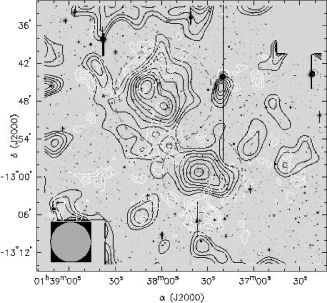
Figure 21: Aperture quadrupole moment map of A 222/223 in an aperture of $3\aas@@fstack{\prime}{2}$ radius, corresponding to the radius of the circle at the lower left corner. The thick white lines are SNR contours for $|Q^{(2)}|$, the lowest contour being at $2$ and higher contours increasing in steps of $0.5$. The aperture quadrupole moment on the ”filament” region reaches a peak SNR of $3.0$. The black lines are the contours of the mass reconstruction. The dashed circles indicate the $r_{200}$ from our best fit NFW models.

Having found in the previous section that aperture quadrupole moments in principle can be used to quantify the presence of a filamentary structure, if we are able to choose the right size of the aperture, we now apply this method to the A 222/223 system. Fig. 21 shows a $|Q^{(2)}|$ map with a weight function with $3\aas@@fstack{\prime}{2}$ radius. The white significance contours show a quadrupole moment signal on the filament that reaches a peak SNR of $3.0$. The filter scale was chosen to be the same in which the aperture mass statistics gave the most significant signal in the intercluster region. The $|Q^{(2)}|$ signal does not fully trace the filament candidate but only the Western part of it and an extension towards the mass peak in the East. The peak SNR is most likely enhanced by the trough at the Western edge of the mass bridge. It is not surprising that the significance of the quadrupole moments on the possible filament is not very high. The aperture mass statistics already gave a relatively low SNR. The AMM statistics uses data within the same aperture as $M_{\mathrm{ap}}$ but gives more information, namely instead of the mass in the aperture, it gives the mass distribution. Being generated from the same information, this naturally comes with a lower SNR.

Several other features – most of them associated with the slopes of the two massive clusters – are also seen in Fig. 21. Interesting in the context of quantifying filaments is the $|Q^{(2)}|$ statistics in the region between A 222 and the newly detected cluster SE of it. Indeed we see a signal with a peak signal-to-noise ratio of $2.7$ extending between the two clusters. The mass reconstruction in Fig. 2 also shows a connection between both clusters but at a level that is dominated by the noise of the $\kappa$-map. The redshift difference between A 222 and the new cluster, inferred from the color-magnitude diagram (Fig. 7), makes it very unlikely that these two clusters are connected by a filament. It is much more probable that we are in the situation depicted by Fig. 16 in which the influence of the two individual clusters leads to a quadrupole moment in the intercluster region.

6 Discussion and conclusions

Based on observations made with WFI at the ESO/MPG 2.2 m telescope we find a clear lensing signal from the Abell clusters A 222 and A 223. Comparing our lensing analysis with the virial masses and X-ray luminosities, we find that A 222/223 forms a very complex system. Mass estimates vary considerably depending on the method. Assuming the best-fit NFW profiles of Sect. 3.2 $M_{200}(\mathrm{A\leavevmode\nobreak\ 222})=3.0^{+0.7}_{-0.8}\times 10^{14}h_{70}^{-1}M_{\sun}$ and $M_{200}(\mathrm{A\leavevmode\nobreak\ 223})=5.3^{+1.6}_{-1.4}\times 10^{14}h_{70}^{-1}M_{\sun}$. The masses of the best-fit SIS models within $r_{200}$ as determined from the NFW fit are higher for both cluster but compatible within their respective error bars: $M_{\mathrm{SIS}}(\mathrm{A\leavevmode\nobreak\ 222})=4.8^{+1.0}_{-1.1}\times 10^{14}h_{70}^{-1}M_{\sun}$ and $M_{\mathrm{SIS}}(\mathrm{A\leavevmode\nobreak\ 223})=7.3^{+1.3}_{-1.4}\times 10^{14}h_{70}^{-1}M_{\sun}$. These mass estimates are considerably lower than those derived from the virial theorem for an SIS model. Using the velocity dispersions from D02 we find $M_{\mathrm{vir}}(\mathrm{A\leavevmode\nobreak\ 222})=9.7^{+1.9}_{-1.6}\times 10^{14}h_{70}^{-1}M_{\sun}$ and $M_{\mathrm{vir}}(\mathrm{A\leavevmode\nobreak\ 223})=12.0^{+2.5}_{-2.1}\times 10^{14}h_{70}^{-1}M_{\sun}$.

The $M/L$ ratios we found in Sect. 4 are lower than the ones determined by D02 of $M/L_{R}=(202\pm 43)\,h_{70}\,M_{\sun}/L_{\sun}$ for A 222 and $M/L_{R}=(149\pm 33)\,h_{70}\,M_{\sun}/L_{\sun}$ within a radius of $1.4\,h^{-1}$ Mpc but agree within the error bars of our values for the $M/L$ ratios determined from the SIS model masses, and in the case of A 223 also with the $M/L$ ratio from the NFW model. Two competing effects are responsible for this difference. First and foremost, the weak lensing masses are lower than the masses D02 used. Second, also the luminosities determined are lower than in D02. This has two reasons. First, D02 analyze the Schechter luminosity function; this allows them to estimate the fraction of the total luminosity they observe, while we limit our analysis to the actually observed luminosity. Also, D02 correct the area available to fainter objects by subtracting the area occupied by brighter galaxies, which might obscure fainter ones. Both differences mean that we probably underestimate the total luminosity of the clusters. Our $M/L$ ratios are already at the lower end of common $M/L$ ratios. A higher luminosity would lead to even lower $M/L$ value making A 222 and A 223 unusually luminous clusters, considering their mass. Although this system is complex and probably still in the process of collapsing, the $M/L$ ratios of both clusters are very similar and do not exhibit variations like those observed by G02 in A 901/902. Variations between mass, optical, and X-ray luminosity are seen on smaller scales in A 223. A 223-N is very weak in the X-ray image, while it is the dominant sub-clump in the mass and optical luminosity density map. The latter may, however, be affected by the color selection that misses many of the unusually blue bright galaxies in A 223, especially in the Southern sub-clump.

The weak lensing mass determination depends on the redshift of the FBG which we assumed to be $\overline{z}_{\mathrm{FBG}}=1$. This assumption is based on the redshift distribution of the Fontana et al. (1999) HDF-S photometric redshift catalog. Changes in the redshift distribution could change the absolute mass scale while leaving the dimensionless surface mass density and hence also the significance of the weak lensing signal unchanged. However, the A 222/223 clusters are at comparably low redshift and changes in $\overline{z}_{\mathrm{FBG}}$ affect the mass scale only weakly. To bring $M_{\mathrm{SIS}}(\mathrm{A\leavevmode\nobreak\ 222})$ to the value of $M_{\mathrm{vir}}(\mathrm{A\leavevmode\nobreak\ 222})$, the mean redshift of the faint background galaxies would have to move to $\overline{z}_{\mathrm{FBG}}=0.3$. This is clearly unrealistic given the depth of our WFI images and the color selection we made. Although we cannot exclude deviations from the redshift distribution of Fontana et al. (1999), it is much more realistic to attribute the differences between virial and weak lensing masses to intrinsic cluster properties.

From the visual impression of the galaxy distribution it is already obvious that this system is far from being relaxed. This can affect the measured masses in several ways: First, the deviation from circular symmetry certainly implies that the line of sight velocity dispersion is not equal to the velocity dispersion along other axes in the clusters. If the clusters are oblate ellipsoid with their major axis lying along the line of sight, the measured velocity dispersions will overestimate the velocity dispersion. Second, if the clusters are not virialized, estimating their masses from the virial theorem of course can give significant deviations from their actual mass. Finally, we could only successfully obtain weak lensing mass estimates with spherical models, which are probably not a good representation of the actual system. Although both clusters are clearly elliptical, fits with SIE models could not reliably reproduce the observed cluster properties. This does not come as a total surprise; King et al. (2002) already noticed that the shear log-likelihood function is much more sensitive to changes in the slope than to a possible cluster ellipticity. The insensitivity of the log-likelihood function to the ellipticity parameters means that the fitting procedure rather changes other cluster parameters than reproducing the actual ellipticity which we see in the parameter-free weak lensing reconstruction. This behavior and the difficulty to accurately fit elliptical models to shear data is confirmed by our simulations in Sect. 5.2. Although our assumption about the dispersion of intrinsic galaxy ellipticities and number density were much more optimistic than justified by our data, we could not recover the ellipticity and orientation of the clusters in the $N$-body simulation.

We found that the concentration parameter $c$ of the NFW profile is poorly constrained if we omit the central regions of the cluster in order to avoid contamination with cluster galaxies. This does not significantly affect the masses determined from fitting NFW profiles and was not of prime importance to the work presented here. From varying the radius of the circles in which shear information was ignored, we saw that galaxies closer to the cluster center constrain the concentration parameter better than those at large distances from the clusters. If one wants to determine concentration parameters more reliably, the fitting procedure has to be extended to include background galaxies close in projection to the cluster centers, while ensuring that faint cluster galaxies do not have a strong influence on the shear signal.

The lensing reconstruction shows a “bridge” extending between both clusters of the double cluster system. We devoted much effort to developing a method that could objectively decide whether this tantalizing evidence is indeed caused by a filament like it is predicted from $N$-body simulations of structure formation. Unfortunately, this was mostly done without success. The aperture quadrupole moment statistics in principle has the power to detect the presence of a filament-shaped structure. To objectively apply it, one however needs to be able to separate clusters from the filaments connecting them. We did not find an objective way to do this and had to resort to subjectively defining the sizes of the apertures used.

We would like to stress that this is not a problem of the weak lensing technique but stems from the fact that the description of the cosmic web as filaments and galaxy clusters is based on the visual impression of $N$-body simulations. Attempts to objectively separate these two components from each other require a mathematical description which we tried to develop in Sect. 5.4. This was mostly unsuccessful because we could not find a procedure that reliably reproduces our visual impression. The visual impression of what a filament is, is often sufficient in simulations or redshift surveys where filaments stretching long distances between clusters are seen. In the case of close pairs of clusters – where we can hope to see filaments with today’s telescopes – a more objective criterion is important, but difficult to find.

We have not addressed the question how to distinguish the aperture quadrupole moment of a filamentary structure from that of a pure double cluster system in Sect. 5.3. We found that the quadrupole moment in a system with a filament exceeds that of a halo-halo system without filament. Closer inspection reveals that the shape of the quadrupole moment in the intercluster region changes if a filament is added to a two halo system. Because one can compute significances for AMM in a limited spatial region, a significant deviation from the expected shape of the quadrupole moment from a pure halo system could possibly be used to overcome this difficulty. This can only work if the signal-to-noise ratio of the aperture quadrupole moment is high. Possibly stacking several cluster pairs could provide a sufficiently high SNR. This could in principle be tested with our $N$-body simulations but is beyond the scope of this paper in which we try to develop a criterion to quantify the evidence for filaments in single systems, like the A 222/223 system at hand.

What can we then say about a possible filament between A 222/223? All observations presented in this work – weak lensing, optical, and X-ray – show evidence for a “filament” between the two clusters. The most compelling evidence probably comes from the number density of color-selected early-type galaxies, which is present at the $7\sigma$ level (Fig. 9). The spectroscopic work of D02 and Proust et al. (2000) confirmed the presence of at least some galaxies at the cluster redshift in the intercluster region. Obtaining a larger spectroscopic sample in the intercluster region would allow us to spectroscopically confirm the significance of this overdensity and could provide insights into the correlation of star formation rates and matter density (e.g. Gray et al. 2004). The X-ray emission between the clusters is aligned with the overdensity in galaxy number and luminosity density. This provides further evidence for a “filament” extending between A 222 and A 223.

The signal level of the possible filament in the weak lensing map Fig. 2 is rather low compared to the clusters. The aperture quadrupole statistics has a signal at the $3\sigma$ level on the filament candidate but this signal may already be contaminated by the outskirts of the cluster in the aperture. The most striking “feature” of the mass bridge seen in the $\kappa$ map is the misalignment with respect to the possible filament seen in the optical and X-ray maps. This can be interpreted in several ways. It could suggest that the surface mass density on the “true filament” defined by the position of the optical overdensity and X-ray emission is below our detection limit and what we see in the $\kappa$ map is a noise artifact. This possibility aside, the observed misalignment can have several causes. First, as we already discussed in Sect. 4, the influence of the many reflection features around the bright star West of A 223 on the weak lensing reconstruction is difficult to determine. It seems that the cluster peaks are shifted preferentially away from the reflection rings. The same could be true for the “filament” in the reconstruction. Second, the position of structures inferred from weak lensing is affected by the noise of the reconstruction. This is especially true for low mass structures and is illustrated by our simulations using SIS models to infer the positional uncertainty of weak lensing reconstructed peaks in Sect. 3.2. It is possible that at least part of the observed misalignment is caused by the noise of the weak lensing method. Finally, one could in principle imagine that the off-set is real and a misalignment of dark and luminous matter is present. This would require complex and possibly exotic physical processes that cause galaxies to form next to a dark matter filament and not in it. At present there is no good observational support for such a scenario. We should note, however, that a misalignment between mass and light is also present in the filament candidate of G02.

As we have not found an objective way to define what a filament in a close double cluster pair is, the question whether what we observe in A 222/223 constitutes a filament or not can also not be answered objectively. Thus, our filament candidate is – in this respect – not very different from those of Kaiser et al. (1998) and G02. The projected virial radii of the clusters marginally overlap. However, (1) the redshift difference between the clusters make an actual overlap of the clusters unlikely; (2) the projected mass in clusters falls off steeply, and weak lensing is currently not capable of mapping the cluster mass distribution out to the virial radius. A signature of a filament should thus already be present inside the virial radius.

The unambiguous weak lensing detection of a filament between two clusters would provide a powerful support for the theory of structure formation and the “cosmic web”. Taking the $3\sigma$ signal of the quadrupole statistics on the filament candidate at face value, an increase of the number of density of FBGs by a factor of $2.8$ could give a $5\sigma$ detection. Such number densities can be reached by $8$ m class telescopes. The A 222/223 system, being only the third known candidate system to host a filament connecting two cluster, would be a good target for such a study. In fact, a weak lensing study of A 222/223 using SuprimeCam at the Subaru telescope is already underway (Miyazaki et al., in preparation).

In addition to the lensing signal from Abell 222 and Abell 223 we found a significant mass peak SE of A 222. This peak coincides with an overdensity of galaxies. The color-magnitude diagram of these galaxies suggest that this newly found cluster is at a redshift of $z\sim 0.4$, but this estimate comes with a considerable uncertainty and requires spectroscopic confirmation. A maximum likelihood fit to the shear data around this mass peak leads to a best-fit SIS model with a velocity dispersion of $728^{+101}_{-120}$ km s^-1. This serendipitous detection again illustrates the power of weak lensing as a tool for cluster searches.

Appendix A Strong lensing features in A 222

Already in 1991 Smail et al. (1991, SEF) found two candidate arclets in the center of A 222. We also see two possible arclets in the center of A 222 displayed in Fig. 22.

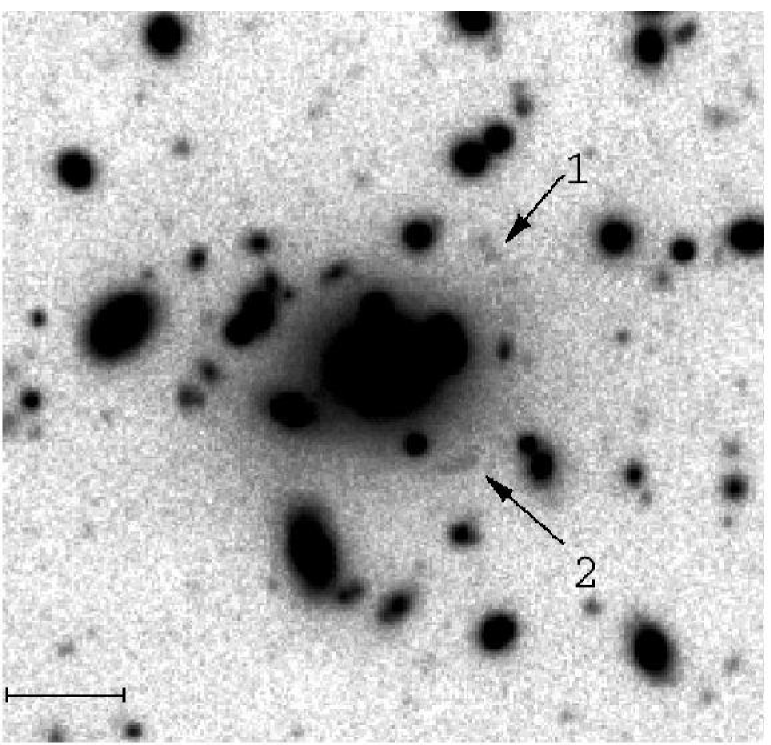
Figure 22: Arclet candidates around the cD galaxy in A 222. North is up and East is to the left. The scale is 10″ long.

Arclet 1 is the same as found by SEF and labeled A 222-1. Unfortunately, SEF’s second candidate is not marked on the plate in their paper, and as SEF give only distances from the cluster center and no position angle we do not know whether their second candidate corresponds to ours. A comparison of the arclet candidate properties between SEF and our candidates is given in table 2.

Table 2: Arclet candidate properties from SEF and our data. The column entries are distance from the center of the cD galaxy, axis ratio, and position angle measured clockwise from the north direction in Fig. 22.

Arc ID	d/arcsec	b/a	pos. angle
SEF
A 222-1	12.2	4.7	-
A 222-2	14.1	2.6	-
this work
arclet 1	12.7	2.8	42°
arclet 2	10.8	3.0	140°

The distance measurements for A 222-1 and arclet 1 are in good agreement but the values for the axis ratio show a clear deviation. The difference may be due to the comparably poor image quality in the work of SEF and blending with the nearby object to the South-West of arclet 1. However, it must also be mentioned that the determination of the axial ratio is relatively uncertain and we estimate its error to be of the order $\simeq 0.6$.

Given the discrepancy between the distance measurements for A 222-2 and arclet 2 it is unlikely that these are the same objects.

Unfortunately, the $V$ band image is not deep enough to show the candidate arclets, so that no color information is available.

Appendix B Multipole moments

Schneider & Bartelmann (1997) define the complex $n$th-order aperture multipole moment as

$$Q^{(n)}\left(\@vec{\theta}_{0}\right)=\int_{0}^{\infty}\mathrm{d}^{2}\@vec{\theta}\;\theta^{n}U(|\@vec{\theta}|)\mathrm{e}^{n\mathrm{i}\varphi}\kappa(\@vec{\theta}_{0}+\@vec{\theta})$$ (8)

with a radially symmetric weight function $U(|\@vec{\theta}|)$. For $n=2$ eq. (8) expresses the aperture quadrupole moment in terms of the surface mass density. Based on this definition, an expression for the aperture moments in terms of shear estimates may be found (Schneider & Bartelmann 1997):

$$Q^{(n)}\left(\@vec{\theta}_{0}\right) = \frac{1}{\overline{n}}\sum_{i=1}^{N}\mathrm{e}^{n\mathrm{i}\varphi_{i}}\times$$ (9)

$$\left\{\theta_{i}^{n}U(\theta_{i})\varepsilon_{\mathrm{t}i}+\mathrm{i}\frac{\theta_{i}^{n}[nU(\theta_{i})+\theta U^{\prime}(\theta_{i})]}{n}\varepsilon_{\times i}\right\}\;,$$

where $\overline{n}$ is the number density of galaxies in the aperture, $(\theta_{i},\varphi_{i})$ are the polar coordinates of the $i$th galaxy with respect to $\@vec{\theta}_{0}$, and $\varepsilon_{\mathrm{t}i}=-\mathcal{R}(\varepsilon_{i}\mathrm{e}^{-2\mathrm{i}\varphi_{i}})$ and $\varepsilon_{\times i}=-\mathcal{I}(\varepsilon_{i}\mathrm{e}^{-2\mathrm{i}\varphi_{i}})$ are the tangential and cross components of the shear estimate, respectively, with respect to $\@vec{\theta}_{0}$. Here $U^{\prime}(\theta)$ is the derivative of the weight function.

We now show that the definition (8) cannot be generalized to non-radially symmetric filters $U(\@vec{\theta})$. We partially integrate eq. (8) with respect to $\varphi$ and obtain

$$Q^{(n)} = \frac{\mathrm{i}}{n}\int_{0}^{\infty}\mathrm{d}\theta\;\theta^{n+1}$$ (10)

$$\int_{0}^{2\pi}\mathrm{d}\varphi\;\mathrm{e}^{n\mathrm{i}\varphi}\left[U(\@vec{\theta})\frac{\partial}{\partial\varphi}\kappa(\@vec{\theta})+\kappa(\@vec{\theta})\frac{\partial}{\partial\varphi}U(\@vec{\theta})\right]\;,$$

where for simplicity we have set $\@vec{\theta}_{0}=0$ without loss of generality. The integral over the first term in this expression can be expressed in terms of the shear in analogy to Schneider & Bartelmann (1997), while we integrate the second term again by parts, this time with respect to $\theta$. This integration over the second term leads to an expression similar to (10) with integrals over two terms; one that can be readily expressed in terms of the shear, the other requiring further integration by parts, and so on. Eventually, the aperture multipole moment can be expressed in terms of the shear as an infinite series of integrals:

$$Q^{(n)} = \int_{0}^{\infty}\mathrm{d}\theta\;\theta^{n+1}\int_{0}^{2\pi}\mathrm{d}\varphi\;\mathrm{e}^{n\mathrm{i}\varphi}U(\@vec{\theta})\gamma_{\mathrm{t}}(\@vec{\theta})$$ (11)

$$+\frac{\mathrm{i}}{1-\frac{\mathrm{i}}{n}}\int_{0}^{\infty}\mathrm{d}\theta\int_{0}^{2\pi}\mathrm{d}\varphi\;\theta^{n+1}\mathrm{e}^{n\mathrm{i}\varphi}U(\@vec{\theta})\gamma_{\times}(\@vec{\theta})$$

$$+\sum_{j=0}^{\infty}\left(\frac{\mathrm{i}}{n}\right)^{j+1}\!\!\int_{0}^{\infty}\mathrm{d}\theta\int_{0}^{2\pi}\mathrm{d}\varphi\;\theta^{n+2}\gamma_{\times}(\@vec{\theta})\frac{\partial^{j+1}}{\partial\theta\partial\varphi^{j}}U(\@vec{\theta})$$

with the requirement on the weight function that

$$\gamma_{\times}\theta^{n+2}\left(\frac{\partial}{\partial\varphi}\right)^{j}U(\@vec{\theta})\rightarrow 0,\;\mathrm{for}\;\theta\rightarrow 0\;\mathrm{and}\;\theta\rightarrow\infty\;,$$ (12)

so that the integrals exist. $\gamma_{\mathrm{t}}$ and $\gamma_{\times}$ are the tangential and cross components of the shear, in analogy to $\varepsilon_{\mathrm{t}}$ and $\varepsilon_{\times}$ above. It turns out that this sum in general does not converge. E.g. for $n=2$ and

$$U(\@vec{\theta})=f(\theta)\left[1+\frac{\epsilon}{2}\left(\mathrm{e}^{2\mathrm{i}\varphi}+\mathrm{e}^{-2\mathrm{i}\varphi}\right)\right]\;,$$ (13)

where $f(\theta)$ is a smooth, positive, and finite function satisfying the condition (12), the sum in eq. (11) oscillates around $0$. This behavior can be understood if we insert (13) into (8) and integrate by parts, while setting $\kappa(\@vec{\theta})$ to a constant value $\kappa_{0}$. The quadrupole moment then depends on $\kappa_{0}$, unless we allow $\theta^{3}f(\theta)$ to be compensated. A constant $\kappa_{0}$ does not influence the shear. Hence, the sum in eq. (11) cannot converge. We thus find that the mass-sheet degeneracy prevents us from computing aperture multipole moments in non-circular apertures.

References

- Abell (1958) Abell, G. O. 1958, ApJS, 3, 211
- Bartelmann & Schneider (2001) Bartelmann, M. & Schneider, P. 2001, Physics Report, 340, 291
- Baugh et al. (2004) Baugh, C. M., Croton, D. J., Gaztañaga, E., et al. 2004, MNRAS, 351, L44
- Bertschinger (1987) Bertschinger, E. 1987, ApJ, 323, L103
- Bertin & Arnouts (1996) Bertin, E. & Arnouts, S. 1996, A&AS, 117, 393
- Bertschinger & Gelb (1991) Bertschinger, E. & Gelb, J. M. 1991, Computers in Physics, 5, 164
- Bond et al. (1996) Bond, H., Kofman, L., & Pogosyan, D. 1996, Nature, 380, 603
- Bruzual & Charlot (1993) Bruzual, A., G. & Charlot, S. 1993, ApJ, 405, 538
- Butcher et al. (1983) Butcher, H., Wells, D. C., & Oemler, A. 1983, ApJS, 52, 183
- Clowe et al. (1998) Clowe, D., Luppino, G. A., Kaiser, N., Henry, J. P., & Gioia, I. M. 1998, ApJ, 497, L61
- Clowe & Schneider (2001) Clowe, D. & Schneider, P. 2001, A&A, 379, 384
- David et al. (1999) David, L. P., Forman, W., & Jones, C. 1999, ApJ, 519, 533
- Davis et al. (1985) Davis, M., Efstathiou, G., Frenk, C. S., & White, S. D. M. 1985, ApJ, 292, 371
- de Lapparent et al. (1986) de Lapparent, V., Geller, M. J., & Huchra, J. P. 1986, ApJ, 302, L1
- Dietrich et al. (2002) Dietrich, J. P., Clowe, D. I., & Soucail, G. 2002, A&A, 394, 395 (D02)
- Doroshkevich et al. (2004) Doroshkevich, A., Tucker, D. L., Allam, S., & Way, M. J. 2004, A&A, 418, 7
- Erben et al. (2003) Erben, T., Miralles, J. M., Clowe, D., et al. 2003, A&A, 410, 45
- Erben et al. (2005) Erben, T., Schirmer, M., Dietrich, J. P., et al. 2005, astro-ph/0501144
- Erben et al. (2001) Erben, T., Van Waerbeke, L., Bertin, E., Mellier, Y., & Schneider, P. 2001, A&A, 366, 717
- Fontana et al. (1999) Fontana, A., D’Odorico, S., Fosbury, R., et al. 1999, A&A, 343, L19
- Gavazzi et al. (2004) Gavazzi, R., Mellier, Y., Fort, B., Cuillandre, J.-C., & Dantel-Fort, M. 2004, A&A, 422, 407
- Geller & Huchra (1989) Geller, M. J. & Huchra, J. P. 1989, Science, 246, 897
- Giovanelli et al. (1986) Giovanelli, R., Myers, S. T., Roth, J., & Haynes, M. P. 1986, AJ, 92, 250
- Gray et al. (2002) Gray, M. E., Taylor, A. N., Meisenheimer, K., et al. 2002, ApJ, 568, 141 (G02)
- Gray et al. (2004) Gray, M. E., Wolf, C., Meisenheimer, K., et al. 2004, MNRAS, 347, L73
- Hoffman & Ribak (1991) Hoffman, Y. & Ribak, E. 1991, ApJ, 380, L5
- Jain et al. (2000) Jain, B., Seljak, U., & White, S. 2000, ApJ, 530, 547
- Joeveer et al. (1978) Joeveer, M., Einasto, J., & Tago, E. 1978, MNRAS, 185, 357
- Kaiser & Squires (1993) Kaiser, N. & Squires, G. 1993, ApJ, 404, 441
- Kaiser et al. (1995) Kaiser, N., Squires, G., & Broadhurst, T. 1995, ApJ, 449, 460
- Kaiser et al. (1998) Kaiser, N., Wilson, G., Luppino, G., et al. 1998, astro-ph/9809268
- Kauffmann et al. (1999) Kauffmann, G., Colberg, J. M., Diaferio, A., & White, S. D. M. 1999, MNRAS, 303, 188
- Keeton & Kochanek (1998) Keeton, C. R. & Kochanek, C. S. 1998, ApJ, 495, 157
- King et al. (2002) King, L. J., Clowe, D. I., & Schneider, P. 2002, A&A, 383, 118
- Klypin & Shandarin (1983) Klypin, A. A. & Shandarin, S. F. 1983, MNRAS, 204, 891
- Möller & Fynbo (2001) Möller, P. & Fynbo, J. U. 2001, A&A, 372, L57
- Monet et al. (1998) Monet, D., Bird A., Canzian, B., et al. 1998, The USNO-A2.0 Catalogue (U.S. Naval Observatory, Washington DC)
- Nicastro (2003) Nicastro, F. 2003, in Maps of the Cosmos, IAU Symposium 216
- Pelupessy et al. (2003) Pelupessy, F. I., Schaap, W. E., & van de Weygaert, R. 2003, A&A, 403, 389
- Pisani (1993) Pisani, A. 1993, MNRAS, 265, 706
- Pisani (1996) —. 1996, MNRAS, 278, 697
- Pogosyan et al. (1998) Pogosyan, D., Bond, J. R., Kofman, L., & Wadsley, J. 1998, in Wide Field Surveys in Cosmology, 14th IAP meeting held May 26-30, 1998, Paris. Publisher: Editions Frontieres, 61
- Press et al. (1992) Press, W. H., Teukolsky, S. A., Vetterling, W. T., & Flannery, B. P. 1992, Numerical recipes in C. The art of scientific computing (Cambridge: University Press, 2nd ed.)
- Proust et al. (2000) Proust, D., Cuevas, H., Capelato, H. V., et al. 2000, A&A, 355, 443
- Schaap & van de Weygaert (2000) Schaap, W. E. & van de Weygaert, R. 2000, A&A, 363, L29
- Schirmer et al. (2003) Schirmer, M., Erben, T., Schneider, P., et al. 2003, A&A, 407, 869
- Schlegel et al. (1998) Schlegel, D. J., Finkbeiner, D. P., & Davis, M. 1998, ApJ, 500, 525
- Schneider (1996) Schneider, P. 1996, MNRAS, 283, 837