X-ray Study of the Intermediate-Mass Young Stars Herbig Ae/Be Stars

Abstract

We present the ASCA results of intermediate-mass pre-main-sequence stars (PMSs), or Herbig Ae/Be stars (HAeBes). Among the 35 ASCA pointed-sources, we detect 11 plausible X-ray counterparts. X-ray luminosities of the detected sources in the 0.5–10 keV band are in the range of log L_X $\sim$30$-$32 ergs s^-1, which is systematically higher than those of low-mass PMSs. This fact suggests that the contribution of a possible low-mass companion is not large. Most of the bright sources show significant time variation, particularly, two HAeBes - MWC 297 and TY CrA - exhibit flare-like events with long decay timescales ($e$-folding time $\sim$ 10$-$60 ksec). These flare shapes are similar to those of low-mass PMSs. The X-ray spectra are successfully reproduced by an absorbed one or two-temperature thin-thermal plasma model. The temperatures are in the range of kT $\sim$ 1$-$5 keV, which are significantly higher than those of main-sequence OB stars (kT $<$ 1 keV). These X-ray properties are not explained by wind driven shocks, but are more likely due to magnetic activity. On the other hand, the plasma temperature rises as absorption column density increases, or as HAeBes ascend to earlier phases. The X-ray luminosity reduces after stellar age of a few$\times$10⁶ years. X-ray activity may be related to stellar evolution. The age of the activity decay is apparently near the termination of jet or outflow activity. We thus hypothesize that magnetic activity originates from the interaction of the large scale magnetic fields coupled to the circumstellar disk. We also discuss differences in X-ray properties between HAeBes and main-sequence OB stars.

1 Introduction

Main sequence stars (MSs) in the intermediate-mass range (2$-$10 M_⊙) exhibit no significant X-ray activity (e.g. Rosner et al., 1985; Berghöfer et al., 1997), due to the absence of X-ray production mechanisms: neither strong UV field to accelerate high-speed stellar winds working in high-mass stars, nor surface convection responsible for magnetic activity working in low-mass stars. Intermediate and high-mass stars in the pre-main-sequence (PMS) stage, called Herbig Ae/Be stars (HAeBes, Herbig, 1960; Waters & Waelkens, 1998) have also neither strong UV fields nor surface convection zones, hence no X-ray emission is predicted for them. Nevertheless the ROSAT and Einstein surveys detected the X-ray emission from significant numbers of HAeBes (Zinnecker & Preibisch, 1994; Damiani et al., 1994). Damiani et al. (1994), using Einstein, detected X-ray emission from 11 HAeBes out of 31 samples. They found that Be stars are more luminous than Ae stars, and suggested that the X-ray luminosity correlates to the terminal wind velocity, but not to the stellar rotational velocity $v_{rot}$ sin $i$. Zinnecker & Preibisch (1994) detected 11 HAeBes out of 21 ROSAT samples. In contrast to the Einstein result, they found no significant difference of X-ray luminosity between Be and Ae stars. They found no correlation of X-ray luminosity to $v_{rot}$ sin $i$, but found a correlation to mass loss rate. Thus both the ROSAT and Einstein results suggested that X-ray emission of HAeBes relates to the stellar winds.

The ASCA spectra from some bright HAeBes (HD 104237, IRAS 12496$-$7650 and MWC 297) exhibited high temperature plasma (kT $\sim$3 keV), while MWC 297 exhibited a large X-ray flare (Skinner & Yamauchi, 1996; Yamauchi et al., 1998; Hamaguchi et al., 2000). Such hot plasma and/or rapid X-ray variability can not be produced by stellar wind. Such properties are usually seen in low-mass stellar X-rays originating from magnetic activity. In fact, magnetic activity of HAeBes may be found in the powerful outflows and jets (Mundt & Ray, 1994).

Wide band imaging spectroscopy between 0.5$-$10 keV first enabled with ASCA is a powerful tool to measure plasma temperatures and time variations. We thus perform a survey of HAeBes using the ASCA archive. From the systematic X-ray spectrum and timing analysis, we study the origin of the X-ray emission from HAeBes with reference to the ROSAT and Einstein results. The combined analysis leads us to an overall picture across the whole pre-main-sequence (PMS) phase of low and intermediate-mass stars.

This paper comprises as follows. The method of target selection is described in Section 2. Data analysis and brief results are summarized in Section 3. Comments on individual sources are in Section 4. The discussion of the X-ray emission mechanism and related phenomena to MS stars are described in Section 5 and 6. Section 7 summarizes results.

2 Target Selection & Data Reduction

We obtained X-ray data from 6 HAeBes, V892 Tau, IRAS 12496$-$7650, MWC 297, HD 176386, TY CrA, and MWC 1080 with our ASCA guest observing programs. We further picked up HAeBe samples from the ASCA archive using the comprehensive catalog compiled by Thé et al. (1994) (above spectral type F in Table i, ii and v) and the recent lists by van den Ancker et al. (1997, 1998). We also analyzed the proto-HAeBe EC95 (Preibisch, 1999), that is not included in the statistical analysis of HAeBe X-ray properties but used for evolutional study of the X-ray emission. The list of the observed HAeBes is given in Table 1. Optical positions in Column 2, 3 and distance in Column 4 are from HIPPARCOS if available (van den Ancker et al., 1997, 1998; Bertout et al., 1999). The ASCA observation log is shown in Table 2.

The fourth Japanese X-ray satellite ASCA, launched in 1993, has four multi-nested Wolter type I X-ray telescopes (XRT), on whose focal planes two X-ray CCD cameras (Solid-state Imaging Spectrometer: SIS) and two gas scintillation proportional counters (Gas Imaging Spectrometer: GIS) are installed (Tanaka et al., 1994). The XRTs have a cusped shape point spread function (psf) with the half power diameter of $\sim$3^′, which is slightly degraded for the GISs by their detector response. The effective area of the four sets of mirrors are around 1400 cm^-2 at 2 keV and 900 cm^-2 at 5 keV. Bandpasses of the SIS and the GIS combined with the XRT are around 0.4$-$10 keV and 0.7$-$10 keV, respectively. The SISs have moderate spectral resolution of $\sim$130 eV at 5.9 keV and field of view (fov) of 20^′ $\times$20^′ with four CCD chips fabricated on each SIS (Burke et al., 1994; Yamashita et al., 1999). A CCD chip needs 4 seconds to be read out, and runs of 1, 2 and 4 chips (corresponding to 1, 2 and 4 CCD modes) need 4, 8 and 16 seconds in an exposure, respectively. After $\sim$1995, spectral resolution of data taken with 2 and 4 CCD modes significantly degraded, which is caused by development of pixel-to-pixel variation of dark current (residual dark distribution: RDD). The clocking and telemetry modes of the SIS detectors are summarized in Column 5. The GISs have energy resolution of $\sim$460 eV at 5.9 keV and wide fov (50^′ diameter) (Ohashi et al., 1996; Makishima et al., 1996). All observations except for PSR J0631 were made with the standard GIS (PH) mode, while a non-standard bit assignment (9-8-8-0-0-0-7) was used for PSR J0631.

We use the ASCA ”revision2” archival data. The data basically do not need further reduction, but the degradation of the SIS data by RDD in the 2 and 4 CCD modes are restored using correctrdd (Dotani et al., 1997). We remove hot and flickering pixels in the SIS using sisclean and select the ASCA grade 0234. The GIS events are selected using gisclean (Ohashi et al., 1996). Both the SIS and the GIS data are screened using the standard criteria, which excludes data in the South Atlantic Anomaly, Earth occultation and high-background regions with low-geomagnetic rigidities. The SIS data with viewing angle less than 20^∘ above the day-earth horizon are also excluded. Analyses are made using the software package FTOOLS 4.2, XIMAGE ver. 2.53, XSPEC ver. 9.0 and XRONOS ver. 4.02.

3 Analysis & Results

3.1 Source Detection

The analysis is basically made in the 0.5–10 keV band for the SIS and the 0.8–10 keV band for the GIS. The low energy threshold for the SIS is set at slightly higher level than those of the onboard discrimination because the low energy efficiency at these levels are degraded by RDD and the event splitting effects can not be fully corrected by correctrdd.

We made X-ray images for both the SIS and the GIS in J2000 coordinate, where the absolute coordinate is corrected by the method in Gotthelf et al. (2000). The positional accuracy for the SIS bright sources should be within $\sim$12^′′. We searched for X-ray sources above 5$\sigma$ detection level around the position of relevant HAeBe. Still possible mis-identification to nearby sources can not be excluded in crowded regions. We checked the ROSAT results in Zinnecker & Preibisch (1994) and Preibisch (1998) and/or retrieved the ROSAT images (Table 3) to confirm the source identifications. To extract the X-ray events for spectral and timing analysis, we normally took a circle of 2.^′5 or 3^′ radius around the relevant source. The background region is selected from the nearby source-free region or at the symmetrical region with respect to a contaminating source, if any. The selected background regions are summarized in Table 4.

For non-detected HAeBes, we determine the 3$\sigma$ upper-limit (99% confidence levels) from a 40^′′ square region for the SIS and a 80^′′ square region for the GIS. The background data are taken from a nearby source-free region with the sosta package in XIMAGE. The upper-limits are converted to fluxies using the PIMMS package assuming an absorbed thin-thermal model with kT = 1 keV, abundance = 0.3 Z_⊙ and N_H converted from A_V (N_H $\sim$2.2 $\times$10²¹A_V cm^-2, Ryter, 1996). The upper-limit flux for retrieving ROSAT data is estimated using the same method as the ASCA data, except that the background is taken from a surrounding 12^′ $\times$12^′ region. ROSAT has narrower bandpass (0.1–2.4 keV) than ASCA, but it has sharper on-axis psf, and therefore is better for source identification especially in a crowded region.

Table 5 and 6 list the detected and non detected sources, respectively. With the ASCA satellite, 11 sources are found above the 5 $\sigma$ threshold. (V921 Sco is excluded due to difficulty in identification.) The detection rate ($\sim$ 31%) is smaller than that of the ROSAT survey ($\sim$ 52%, Zinnecker & Preibisch 1994), due mainly to the higher detection threshold to eliminate contamination from nearby bright sources (e.g. AB Aur, HD 97048 and Z CMa). A few embedded sources (e.g. MWC 297 and IRAS 12496-7650) are however detected for the first time in X-rays by ASCA, thanks to its hard X-ray imaging capability.

3.2 Timing Analysis

We made light curves in the full energy range by subtracting background. The time bin is typically 2048 sec but it is longer for weak sources. The error of each bin is estimated by the Gaussian approximation. Typical net counts per bin of combined SIS and GIS light curves are around 80 counts/bin. We fit the light curves with a constant-flux model using the chi-square method, and find time variable sources with 96% confidence.

Table 7 shows the result of the timing analyses. Four (or five if we include merged light curves of TY CrA and HD 176386 (TYHD)) among twelve detected sources (36–45%) were variable. If we exclude sources with total net counts less than 1000 photons, half (or 3/4 including TYHD) are variable.

3.3 Spectra

We fit spectra with an absorbed thin-thermal plasma model (the MeKaL plasma code, Mewe et al. 1995). The response matrixes for the SIS were made with sisrmg ver. 1.1, while a standard one was used for the GIS. The ancillary response function for both were made with ascaarf ver. 2.81. Chemical abundances are basically fixed at 0.3Z_⊙, following the typical value for the stellar X-rays (e.g. OB stars, Kitamoto & Mukai 1996; Kitamoto et al. 2000; low-mass MSs, Tagliaferri et al. 1997; low-mass PMSs, Yamauchi et al. 1996; Kamata et al. 1997; Tsuboi et al. 1998).

Spectra for most sources except HD 104237 and HD 200775 were fit with either an absorbed one-temperature (1T) or two-temperature (2T) thin-thermal (MeKaL) model (with a Gaussian component for VY Mon) with 90% confidence (Table 8). Unacceptable fits of HD 104237 and HD 200775 seem to be caused by small structures in the spectra, which might be unknown emission lines or absorptions. The best-fit temperature ranges between kT $\sim$1$-$5 keV, which is significantly higher than the X-ray temperature of MS OB stars (kT $<$1 keV, e.g. Corcoran et al., 1994).

4 Comments on Individual Sources

This section provides observational details of each detected source: i.e. stellar characteristics and ASCA results of imaging, timing and spectral analysis.

4.1 V892 Tau

V892 Tau (Elias 3-1) is located in the L1495E dark cloud. The stellar parameters are open to dispute; Strom & Strom (1994) quoted it as a B9 star of L_bol $\sim$64.3 L_⊙, while Zinnecker & Preibisch (1994) quoted it as an A6e star of L_bol $\sim$38 L_⊙. It has a circumstellar disk of $\sim$0.1 M_⊙ (di Francesco et al., 1997). There is a companion star (Elias I NE) at $\sim$4^′′ northeast from V892 Tau, which would be a weak line T-Tauri star (WTTS) with L_bol $\sim$0.3 L_⊙ (Skinner et al., 1993; Leinert et al., 1997; Pirzkal et al., 1997). Strom & Strom (1994) first reported the X-ray emission from V892 Tau (log L_X $\sim$30 ergs s^-1). Zinnecker & Preibisch (1994) measured a plasma temperature of $\sim$2.3 keV and hydrogen column density of $\sim$4.8 $\times$10²¹ cm^-2.

V892 Tau is detected as the strongest source in the 12^′ $\times$12^′ square field (Figure 1a). The SIS image shows two other X-ray sources: V1023 Tau at $\sim$2^′ northeast from V892 Tau and V410 X-ray 7 at 30^′′ southeast, which is only obviously seen in the soft band image (0.55$-$2 keV). V410 X-ray 7 is a reddened M0.5 PMS star (Briceño et al., 1998), from which ROSAT detected an X-ray flare (Stelzer et al., 2000). Because the GIS does not resolve V1023 Tau from V892 Tau, we only use the SIS for latter analysis. V892 Tau and V410 X-ray 7 strongly merge together so that V410 X-ray 7 is included in the source region of V892 Tau. The light curve in the total band (Figure 1b) seems to fluctuate by a factor of two, but it accepts a constant model within 90% confidence level, which suggests that neither V892 Tau nor V410 X-ray 7 showed variation. The spectrum can be reproduced by an absorbed 1T thin-thermal model (1T model in Table 8), but it includes a component from V410 X-ray 7. As we see in the SIS hard band image, hard X-ray emission from V410 X-ray 7 is negligible. Because the high energy part of the X-ray emission determines the plasma temperature, we think that the temperature derived in the 1T model represents the temperature of V892 Tau. On the other hand, in the soft band image (0.55$-$2 keV), V410 X-ray 7 is as bright as V892 Tau, which means that the soft X-ray flux of V892 Tau is half of that of the 1T model. When we only change N_H parameter of the 1T model to fit the condition, N_H of V892 Tau is $\sim$1.8$\times$10²² cm^-2. The residual component, which would be attributed to V410 X-ray 7, can be successfully fit by another absorbed 1T model (2T model in Table 8 and Figure 1c).

4.2 V380 Ori

V380 Ori is a B9–A0 star of 3.3$-$3.6 M_⊙ with small amplitude variability (Hillenbrand et al., 1992; Böhm & Catala, 1995; Rossi et al., 1999; Herbst & Shevchenko, 1999; Rossi et al., 1999). It has a companion star 0.^′′15 from the primary (Corporon & Lagrange, 1999). X-ray emission was detected with Einstein and ROSAT (log L_X $\sim$ 31.0$-$31.3 ergs s^-1, Pravdo & Marshall 1981; Zinnecker & Preibisch 1994). From the Einstein data, the plasma temperature and column density are $\sim$1.1 keV and 7.4$\times$10²¹ cm^-2, respectively (Damiani et al., 1994).

V380 Ori is detected as a relatively faint source (Figure 2a). It is near the edge of the GIS fov (4^′ inside from the edge) so that the psf is less sharp. The light curve shows no apparent variability. The spectral fitting (see Figure 2b) shows relatively high plasma temperature ($\sim$3.2 keV) though the uncertainty (0.7 $-$ 11.0 keV) is large. The luminosity (log L_X $\sim$31.2 ergs s^-1) is about the same as that in the Einstein and ROSAT observations.

4.3 VY Mon & CoKu VY Mon/G2

Both VY Mon and CoKu VY Mon/G2 are members of the Mon OB1 association (Cohen & Kuhi, 1979; Testi et al., 1998). VY Mon is a O9$-$B8 star in very young phase ($\sim$5$\times$10⁴ years) with Algol-type variability and large IR excess (see Casey & Harper, 1990; Thé et al., 1994; Testi et al., 1999). CoKu VY Mon/G2 is a candidate Herbig Ae star (Thé et al., 1994). Damiani et al. (1994) reported X-ray emission from VY Mon and/or CoKu VY Mon/G2 with Einstein in the hard band (S/N $\sim$2.5).

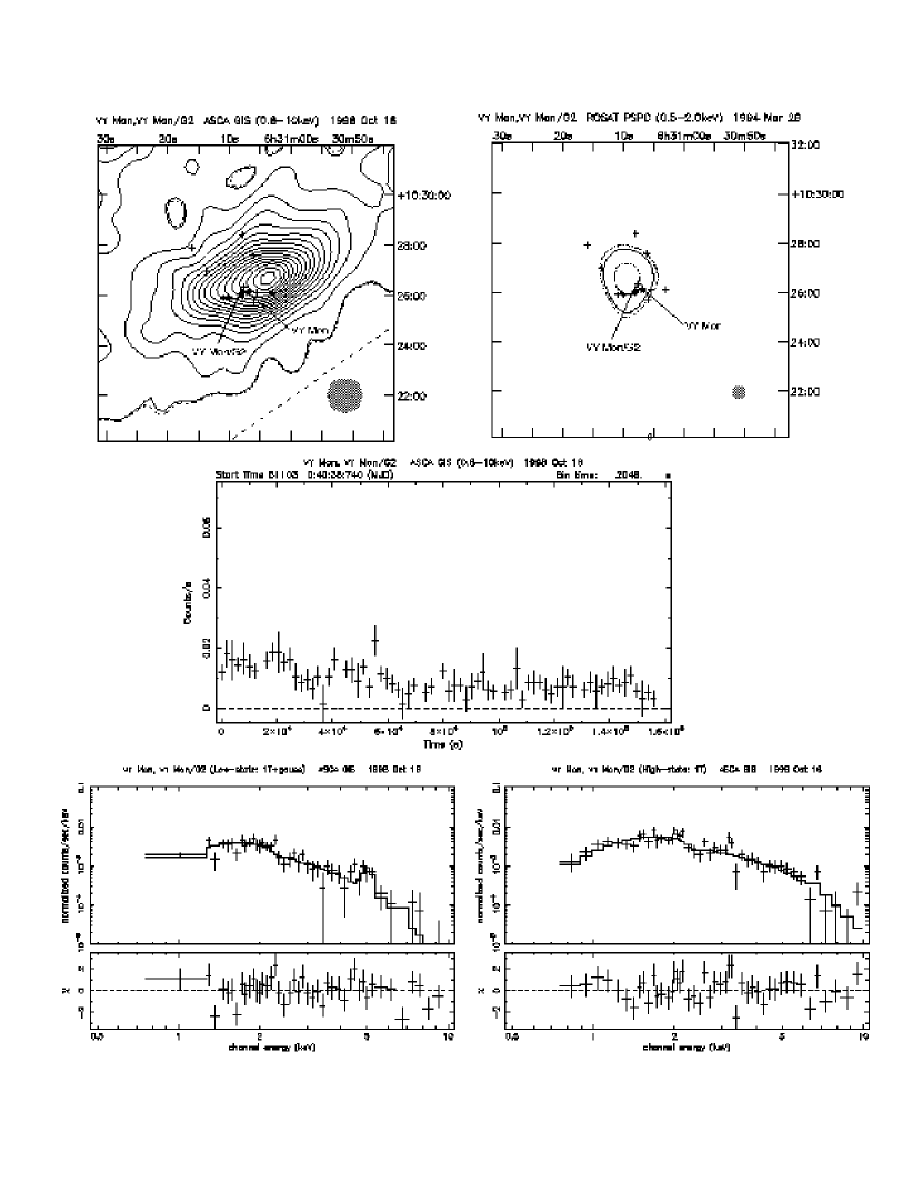
Figure 3: a: ASCA GIS image of the VY Mon field (top left panel) and ROSAT PSPC image of the VY Mon field (top right panel). The star marks are VY Mon (right) and CoKu VY Mon/G2 (left), respectively. b: GIS light curves of VY Mon (middle panel). c: GIS spectra of VY Mon (bottom left panel: LS, bottom right panel: HS).

The GIS detects an X-ray source around VY Mon and CoKu VY Mon/G2 at a large off-axis angle ($\sim$20^′), where the absolute position uncertainty is poorly calibrated (a few arc-minutes) (Figure 3a left). We thus used a ROSAT PSPC image for source identification (Figure 3a right). Though all four ROSAT observations has relatively large off-axis angle of the source ($\sim$30^′), where 68% of source photons falls within a $\sim$1^′ radius circle, VY Mon and/or CoKu VY Mon/G2 can be the counterpart of the X-ray source. The ASCA light curve (Figure 3b) gradually decreases with small fluctuations and becomes almost constant after $\sim$6$\times$10⁴ sec. We thus define the phase before 6$\times$10⁴ sec as the high state (HS) and the phase after as the low state (LS). The low state spectrum has an enhancement at around 5 keV (left panel of Figure 3c). An absorbed 1T model with a Gaussian component at $\sim$5.1 keV has an acceptable fit in 90% confidence level, but there is no corresponding emission line of abundant elements at the measured energy (e.g. Ca, Fe). We also tried an additional thermal model, but it does not reproduce the strong dip feature at $\sim$5.3 keV. The origin of the line emission is unknown. On the other hand, the high state spectrum (right panel of Figure 3c) accepts an absorbed 1T model with very high plasma temperature ($\sim$6 keV). The X-ray luminosity (log L_X $\sim$$32.2$ ergs s^-1) is one of the largest among our samples. VY Mon forms a small cluster. The X-ray emission could be from the assembly of cluster members. However, we should note that N_H does not change between the HS and LS, and corresponds to the A_V ($\sim$1.6^m) of CoKu VY Mon/G2.

4.4 HD 104237

HD 104237, located in the Chamaeleon III dark cloud, is the brightest HAeBe star in the sky (V =6.6^m, Hu et al., 1991). It has the spectral type A4e and would be slightly older than other star HAeBe stars (Age $\sim$10^6.3 years, Knee & Prusti, 1996; van den Ancker et al., 1998). The ASCA observation of HD 104237 is described in Skinner & Yamauchi (1996) in detail.

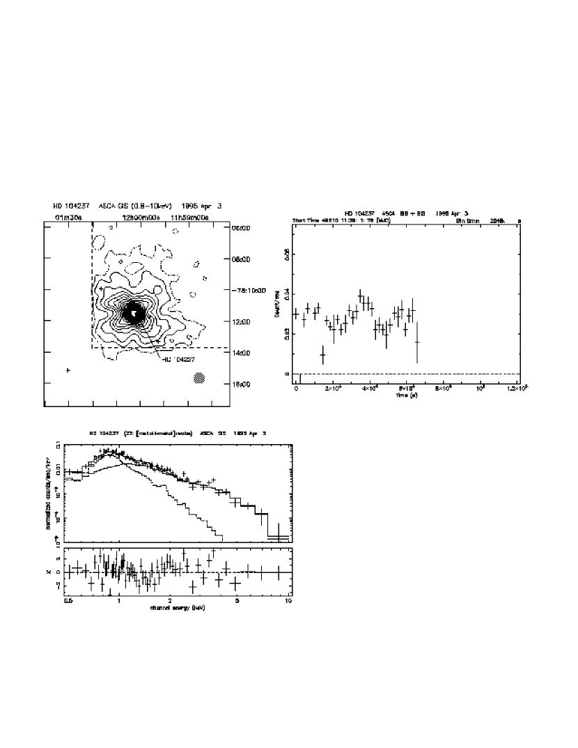
Figure 4: a: SIS image of HD 104237 (top left panel). b: Light curves of HD 104237 (top right panel). c: SIS spectrum of HD 104237 fit by a commonly absorbed 2T model (2T model in Table 8, bottom left panel).

X-ray emission is detected at the position of HD 104237 (Figure 4a). The light curve (Figure 4b) seems to vary periodically and rejects a constant model. The spectrum (Figure 4c) needs at least 2T components, which still seem to have small deviation. Skinner & Yamauchi (1996) succeeded in reproducing the SIS spectrum by 2T models, but we do not succeed in reproducing both the SIS and GIS spectra simultaneously, though we do not find any systematic difference between the spectra. We also tried to fit the spectra by three models, commonly absorbed 2T model with free elemental abundance, 2T model with different N_H, and commonly absorbed 3T model, but the reduced $\chi^{2}$ value did not improve. The large $\chi^{2}$ seems to be caused by weak spectral features (e.g. emission lines). In the discussion section, we refer the physical parameters of HD 104237 to the commonly absorbed 2T model.

4.5 IRAS 12496$-$7650

IRAS 12496$-$7650 is an embedded Herbig Ae star (Hughes et al., 1989) and is the most luminous far-infrared source in the Chameleon II cloud. The ASCA observation is described in Yamauchi et al. (1998).

The GIS image is shown in Figure 5a. The X-ray spectrum (Figure 5b) shows very large absorption of about N_H $\sim$ 10²³ cm^-2, which is more than five times of the N_H converted from the A_V (Hughes et al., 1991). The absorption column is the largest among our sample.

4.6 HR 5999

HR 5999 is a variable A5-7e star with age of 5$\times$10⁵-year-old located in the center of the Lupus 3 subgroup (van den Ancker et al., 1998; Tjin A Djie et al., 1989). It is thought to have an accretion disk (e.g. Thé et al. 1996), which might cause photometric and spectral variations. It also has a close companion at 1.^′′3 apart (Rossiter 3930, Stecklum et al. 1995), probably a T-Tauri star (TTS). The X-ray emission of HR 5999 was detected with ROSAT (Zinnecker & Preibisch, 1994).

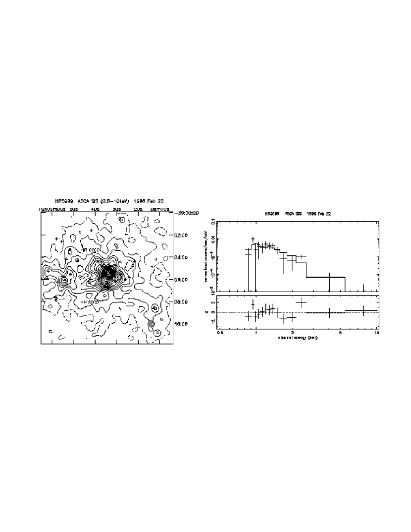
Figure 6: a: SIS image of HR 5999 (left panel). b: SIS spectrum of HR 5999 (right panel).

HR 5999 is fainter and hidden in the psf wings of the intermediate-mass young peculiar star HR 6000. The peak is only recognized in the SIS image (not clear in Figure 6a). To cancel out contamination from HR 6000, we selected a background region symmetric with respect to HR 6000. We do not find any systematic difference in light curve and spectrum between SIS0 and SIS1, which would mean that contamination from HR 6000 is satisfactorily removed. Net event counts within a very small ellipse centered at HR5999 (see Table 4) is around 50% of total counts of the source region. The SIS spectrum of HR 5999 is reproduced by an absorbed 1T thermal model (Figure 6b). The N_H error range ($<$1.2$\times$10²² cm^-2) includes the N_H converted from A_V ($\sim$0.5^m). The temperature is consistent with the hot component seen in the ROSAT spectrum (1T model in Table 8), and become closer to it by assuming the same N_H as in the ROSAT analysis (1T^F model in Table 8, Zinnecker & Preibisch, 1994). The consistency between N_H and A_V and larger L_X than in low-mass stars (see discussion 5.1) suggests that the detected X-ray emission is from HR 5999.

4.7 V921 Sco

V921 Sco (CoD $-$42^∘ 11721) is located in the galactic plane [($l,b$) = (343.35, $-$0.08)]. Some papers classify it as a supergiant (e.g. Hutsemékers & van Drom 1990). The distance to V921 Sco has large uncertainty from 200 pc to 2.6 kpc (Pezzuto et al., 1997; Brooke et al., 1993). We adopt the distance of 500 pc derived from a spectral analysis with the ISO$-$SWS (Benedettini et al., 1998).

A weak X-ray source is detected on the GIS image (Figure 7a). The source is seen as two marginal humps in the SIS, which might mean that the X-ray emission is from multiple nearby sources. Actually V921 Sco, which is in the crowded region on the galactic plane, have $\sim$50 2MASS sources within 1^′ though some of them could be nebulae. We thus show the result of timing and spectral analysis, but do not include the source for studies in the discussion sections. The GIS spectrum (Figure 7b) can be reproduced by an absorbed 1T model with strong absorption (N_H $\sim$5$\times$10²² cm^-2). The N_H is significantly higher than N_H converted from its A_V (N_H $\sim$1.6$\times$10²² cm^-2), though it is consistent with N_H derived from a millimeter survey ($\sim$10²³ cm^-2, Henning et al., 1998).

4.8 MWC 297

MWC 297 is a highly reddened star with extremely strong Balmer and silicate lines. Hillenbrand et al. (1992) reported that MWC 297 is a PMS star with the spectral type of O9 at a distance of 450 pc and age of $\sim$3$\times$10⁴ years. Drew et al. (1997), however, suggested it to be a B1.5 zero-age main-sequence (ZAMS) star at the distance of $\sim$ 250 pc. They also argued that MWC 297 is a rapid rotator with $v_{rot}$ sin $i\sim$ 350 km s^-1. The ASCA observation of MWC 297 is described in Hamaguchi et al. (2000). Here, the X-ray luminosity is smaller than that in Hamaguchi et al. (2000) because we assume a distance of 250 pc.

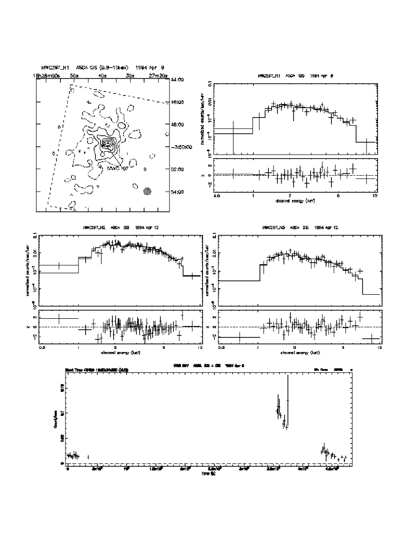
Figure 8: a: SIS image of the MWC 297 field in ”MWC 297 1” (top left panel). The count rate per solid-line is 0.2 cnts pixel^-1. b: Light curve of MWC 297 (bottom panel). c: SIS spectra of MWC 297 in the ”MWC297 1, 2 and 3” (top right, middle left, and middle right panels, respectively).

A point-like X-ray source is detected in three observations spanning 5 days. Figure 8a shows the SIS image from the 1st observation (MWC297 1). We also checked a ROSAT observation of the MWC 297 field (exposure $\sim$1 ksec), but we found no X-ray source in the field. The combined light curves of the three observations (Figure 8b) show that the X-ray flux in the first observation is constant, but increased by a factor of five at the beginning of the second observation, then gradually decreased exponentially to nearly the same flux of the pre-flare level by the end of the third observation with an $e$-folding time $\sim$ 5.6 $\times 10^{4}$ sec. SIS spectra of all observations are separately displayed in Figure 8c. The absorption column $\sim$2.4$\times$10²² cm^-2 did not change during the observations. The plasma temperature in the quiescent phase of 3.4 keV increased to 6.5 keV during the flare and then decreased to 3.4 keV. The flare peak was missed; we only detected X-rays after the on-set of the flare. Thus, the peak luminosity is log L_X $\gtrsim$ 32.1 ergs s^-1, which is the maximum at the beginning of the second observation. A giant X-ray flare from the early MS star $\lambda$ Eridani (B2e) was detected by ROSAT (Smith et al., 1993). The star would be young and would not be a classical Be star. The flare detected on MWC297 might have some relation in mechanism to $\lambda$ Eridani.

4.9 TY CrA / HD 176386

TY CrA and HD 176386 belong to the R CrA cloud and illuminate the reflection nebula NGC 6726/7 (Graham, 1991). TY CrA is a detached Herbig Be eclipsing binary consistency of a 3.16M_⊙ primary star near ZAMS and a 1.64M_⊙ secondary star with an orbital period of $\sim$2.889 days (Kardopolov et al., 1981; Casey et al., 1993, 1995, 1998). Both stars are $\sim$3$\times$10⁶-year-old. The lack of infrared excess indicates absence of an optically thick disk (Casey et al., 1993). It shows non-thermal radio emission (Skinner et al., 1993). The X-ray emission is detected by Einstein and ROSAT. Damiani et al. (1994) measured the plasma temperature at $\sim$1 keV and the absorption column density at $\sim$ 5.5$\times$10²¹ cm^-2. On the other hand, HD 176386 is a B9.5 star close to the ZAMS with mid-infrared excess but no H$\alpha$ emission reported (2.8$\times$10⁶-year-old, Bibo et al., 1992; Grady et al., 1993; Prusti et al., 1994; Siebenmorgen et al., 2000).

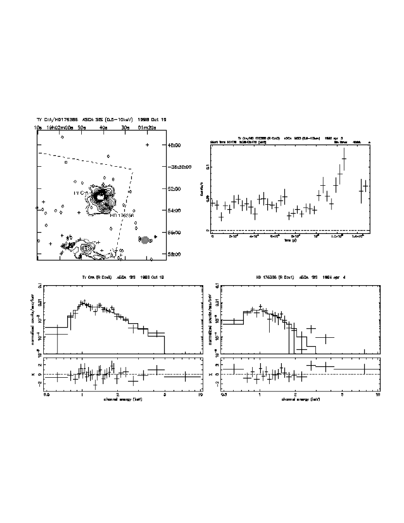
Figure 9: a: SIS image of the TY CrA/HD 176386 field in Oct 1998 (R CrA6, top left panel). b: GIS light curves of TY CrA + HD 176386 (R CrA3 top right panel). c: SIS spectra of TY CrA (R CrA 6, bottom left panel) and HD 176386 (R CrA 1, bottom right panel)

Both TY CrA and HD 176386 exhibit X-ray emission (Figure 9a). We focus on the SIS data taken in 3 observations (R CrA 1, 4 and 6) because the GIS cannot resolve TY CrA and HD 176386, but the SIS marginally does. We selected a background at the symmetrical region with respect to each source to cancel contamination from each other. All light curves are constant in each observation, and the average flux does not change between observations. Spectra of both TY CrA and HD 176386 can be fit by an absorbed 1T model (Figure 9c). For the three observations, the best-fit column density and plasma temperature for TY CrA are 3$-$6$\times$10²¹ cm^-2 and 1$-$2 keV respectively, which are the same as the Einstein result (Damiani et al., 1994). The fits to the HD 176386 spectrum have two local $\chi^{2}$ minima, among which smaller N_H ($<$2$\times$10²¹ cm^-2) is consistent with the A_V. The plasma temperature is around 1$-$2 keV. On the other hand, at the end of R CrA 3 in which only GIS data is available and hence X-ray emission from TY CrA and HD 176386 is merged together, we see a flare like variation with long rise time ($\sim$10 ksec, see also Table 9) as a stellar flare (Figure 9b). We define the high flux state HS and the other LS, and tentatively fit the spectra by an absorbed 1T model. Then the best-fit plasma temperature is slightly higher during HS (kT $\sim$3.0 keV) with respect to LS (kT $\sim$2.6 keV). Because the rise time-scale is too long for a normal stellar flare, the flare might relate to binary interaction. The peak came after 80 ksec of the eclipse of the primary star, equivalent to $\sim$120^∘ rotation of the binary system, when we see $\sim$2/3 of the surface of the companion facing the primary star. The flare may occur on an active spot of the companion at the root of inter-binary magnetic field.

4.10 HD 200775

HD 200775 is a B2.5e star illuminating the reflection nebula NGC 7023 (van den Ancker et al., 1998; Benedettini et al., 1998). It is in a biconical cavity that has been swept away by energetic bipolar outflows, but there is no evidence of ongoing outflow activity (Fuente et al. 1998). Its age is estimated to be $\sim$2$\times$10⁴ years from the HR diagram, but it might be 2 $\times$10⁷ year-old in the post main-sequence stage (van den Ancker et al., 1997). HD 200775 has a companion star 2.^′′25 apart ($\Delta$K = 4.9^m, Li et al., 1994; Pirzkal et al., 1997). Damiani et al. (1994) detected strong X-ray emission with Einstein (log L_X $\sim$31.9 ergs s^-1) and measured N_H $\sim$5$\times$10²¹ cm^-2 and kT $\sim$0.8 keV.

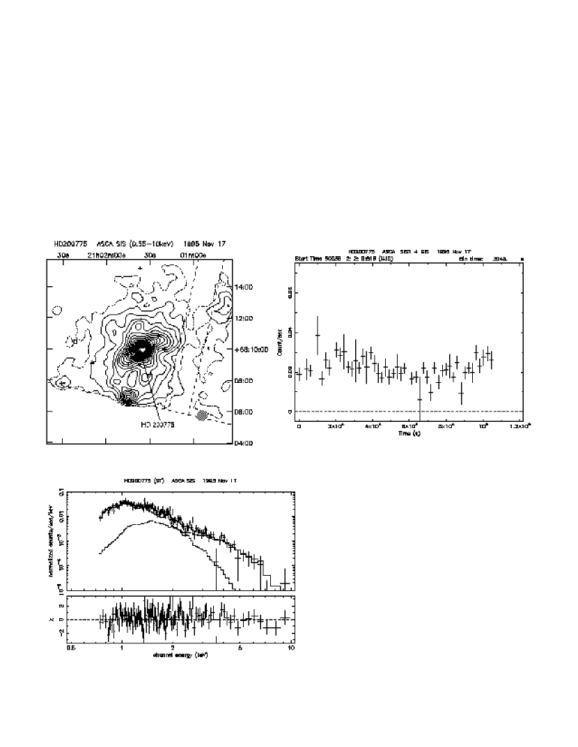
Figure 10: a: SIS image of HD 200775 (top left panel). b: Light curves (SIS1+GIS) of HD 200775 (top right panel). c: SIS spectrum of HD 200775 fit by an absorbed 2T model (bottom left panel).

A point-like source was detected at the position of HD 200775 (Figure 10a). The SIS0 light curve has a spike at about 9.3 $\times$10⁴ sec, which is probably an instrumental artifact. The other light curves (SIS1, GIS) show marginal flux increases around 2, 4 and 10$\times$10⁴ sec, and the light curve rejects a constant model above 96% confidence level. (Figure 10b). The spiky event does not have significant counts so that we use all the SIS and GIS data for spectral fitting (Figure 10c). An absorbed 1T model is rejected over 99.9% confidence. An absorbed 2T model with common N_H improves the reduced $\chi^{2}$ value to 1.15 and is accepted above 90% confidence. However, the N_H value ($\sim$9$\times$10²¹ cm^-2) is two times as large as the converted N_H from visual extinction of HD 200775 (A_V $\sim$1.9^m). Marginal bumpy features are present in the 2$-$4 keV band. We thus tried these two models: (i) 2T thermal model with a free abundances, (ii) 1T thermal and hard power-law model. In the model (i), the metal abundance is slightly larger (0.39 solar) than the fixed abundance (0.3 solar), but the model fit does not improve. On the other hand, the best-fit N_H of the model (ii) is $\sim$4$\times$10²¹cm^-2, which is almost equal to the N_H converted from A_V though we do not have physical interpretation to explain the power-law component.

4.11 MWC 1080

MWC 1080 is an early A type star with A_V $\sim$4.4^m(Yoshida et al., 1992). The distance is 2.2–2.5 kpc from UVBR photometry of neighboring MS stars (Grankin et al., 1992) and kinematic distance of ¹³CO molecular line (Cantó et al., 1984). It forms a multiple system of a HAeBe primary, a plausible HAeBe companion (0.^′′7) and another companion (4.^′′7), with eclipse events at $\sim$2.887 days (Grankin et al., 1992; Leinert et al., 1997; Pirzkal et al., 1997). It has CO molecular outflow and ionizing winds up to 1000 km s^-1 (Cantó et al., 1984; Yoshida et al., 1992; Leinert et al., 1997; Benedettini et al., 1998). The X-ray emission was detected with ROSAT (Zinnecker & Preibisch, 1994, log L_X $\sim$32 ergs s^-1).

An X-ray source was detected near MWC 1080 (Figure 11a). The light curves (Figure 11b) seem to oscillate periodically by $\sim$40 ksec, but this is not statistically significant. The orbital phase during the observation is $\phi=$ 0.39 to 0.74 according to the ephemeris by Grankin et al. (1992). The secondary eclipse occurs at 3$\times$10⁴ sec, but it is not observed in the X-ray light curve. The light curves do not show evidence that binarity affects the observed X-ray emission of MWC 1080. The spectrum (Figure 11c) can be reproduced by an absorbed 1T model. The temperature is extremely high (kT $>$3.8 keV) and the absorption column density (N_H $\sim$10²² cm^-2) is consistent with A_V. The spectrum has an excess around 6–7 keV. When we include a Gaussian model with $\sigma$= 0.0, the center energy is 6.4 (6.2–6.6) keV, which corresponds to the iron fluorescent line. On the other hand, an absorbed 1T model with the free abundance parameter has abundance of 0.8 solar, which is mainly determined from Helium-like Fe-K line emission. The residual still seems to have systematic patterns though the model is accepted $>$90% confidence. A commonly absorbed 2T model or soft 1T + power-law model compensate the pattern slightly better, but the best-fit N_H ($\sim$5$\times$10²² cm^-2) is large and luminosity of the best-fit model is unrealistically high for stellar X-ray emission ($>$10³⁶ergs s^-1).

4.12 EC 95

Preibisch (1998) first reported constant X-ray emission from EC 95. From near-infrared spectroscopy, Preibisch (1999) determined EC 95 as an extremely young intermediate-mass star (Age $\sim$2$\times$10⁵ years; $M\sim$4 M_⊙), a so called proto-HAeBe. The very high visual extinction (A_V $\sim$25$-$35^m) made them suspect that the source has a large intrinsic X-ray luminosity of about log L_X $\sim$33 ergs s^-1. Radio observations have detected a point-like source, SH 68-2, within the error circle of EC 95 (Rodriguez et al., 1980; Snell & Bally, 1986; Smith et al., 1999), showing gyrosynchrotron emission suggesting presence of a magnetosphere.

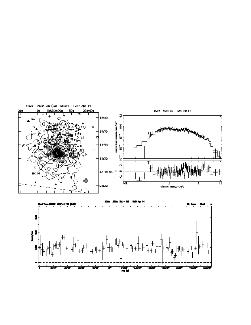
Figure 12: a: SIS image of the EC 95 field (top left panel). b: Light curves of EC 95 (bottom panel). c: SIS spectrum of EC 95 (top right panel).

A point-like source is detected within the error circle of EC 95 (Figure 12a). The nearest ROSAT X-ray source is 1.^′5 apart (Preibisch, 1998). ASCA would see the same source. The light curves show flare-like small fluctuations and reject a constant model (Figure 12b). Spectra of the SIS and GIS (Figure 12c for the SIS) are inconsistent in absolute flux. The SIS flux calibration is less reliable due to CCD degradation. We independently varied the model normalizations, and find an acceptable result. The flux is derived from the GIS data. The plasma temperature is quite high (kT $\sim$3.9 keV). N_H is large but about one fourth of the A_V ($\sim$36^m) converted N_H. The luminosity (log L_X $\sim$31.7 ergs s^-1) is therefore about an order of mag smaller than the ROSAT estimate.

5 X-ray Emission Mechanism

5.1 Could the X-ray Emission Come from a Low-Mass Companion?

More than 85% of HAeBes are visible or spectroscopic binaries (Pirzkal et al., 1997), whose companions could be low-mass stars, i.e. TTSs or protostars. Low-mass stars are known to emit strong X-rays compared with their faint optical and IR emission (L_X/L_bol up to 10^-3). We thus evaluate as whether the X-ray emission observed with ASCA could come from low-mass stars. Stelzer & Neuhäuser (2001) reports that, in the Taurus Auriga region, CTTSs and WTTSs with log L_X $\gtrsim$30 ergs s^-1 are around 5% and 25%, respectively. Multiplying the binary ratio, around 4% and 20% of the X-ray emission with log L_X $\gtrsim$30 ergs s^-1 could be really from low-mass companions. ASCA detected sources have log L_X $\gtrsim$ 30 ergs s^-1 and the detection rate is $\sim$30%. Contribution of the companion could be non-negligible if the companions follow the luminosity function of WTTSs. However, considering that the primary star and its companion tend to have similar ages (e.g. see Casey et al. (1998) for TY CrA), CTTSs with the similar ages to HAeBes ($\sim$10⁶-year-old) might be more appropriate for this estimate, then the contribution of the companion in our sample would be negligible. While there are almost no TTSs above 10³¹ ergs s^-1, therefore the X-ray emission would be responsible for the primary (i.e. early-type) star.

5.2 X-ray Properties

The X-ray properties of HAeBes and their relation to the stellar parameters may provide further insight into the origin of the X-ray emission. In this section, we examine the relation of L_X to other stellar parameters such as L_bol, T_eff and v_rot sin $i$, the X-ray time variability and the plasma temperature. We then compare the properties with those of low-mass and high-mass stars. In the discussion of X-ray luminosity, we included ROSAT samples of HAeBes (Zinnecker & Preibisch, 1994). Their L_X in the ASCA band (0.5–10 keV) is estimated by assuming an absorbed thin-thermal model with kT = 2 keV, abundance = 0.3Z_⊙ and N_H converted from A_V (Ryter, 1996). The errors are put between half and factor of two of their L_X to allow for uncertainty of kT $\sim$0.5$-$4 keV. The photon statistical errors are basically much smaller than this error range. Whereas, we also include EC 95 and SSV 63E+W as candidates of proto-HAeBes. SSV 63E+W is either a Class I protostar candidate SSV 63E or W in the Orion cloud. Zealey et al. (1992) mention that SSV 63E may have mass 1.5M_⊙ $<M<$5 M_⊙ assuming age less than 10⁶-years at a distance of 460 pc. The X-ray emission is reported by Ozawa et al. (1999). On the other hand, we did not include V921 Sco in the sample.

Figure 13a shows the L_X $vs.$ L_bol diagram. In our HAeBe samples ranging between 33 $<$log L_bol ergs s^-1 $<$38, the log L_X/L_bol ratio is between $-$4 and $-$7. The ratio is above the range of massive MS stars ($-$6 $\sim-$8), and rather close to, but slightly different from, that of low-mass stars (up to $-$3) (e.g. Gagné et al., 1995). The L_X/L_bol ratio of proto-HAeBe is close to $-$3. This might suggest that X-ray activity is enhanced in the very youngest stars (see also discussion in the section 5.3). Figure 13b shows the dependence of log L_X/L_bol on log T_eff. The log L_X/L_bol increases as log T_eff decreases, which resembles the trend of X-ray sources in the Orion cloud (Fig. 8 in Gagné et al., 1995). Figure 13c shows the log L_X/L_bol dependence on $v_{rot}$ sin $i$ (Grady et al., 1993; Böhm & Catala, 1995; Drew et al., 1997; Casey et al., 1998; van den Ancker et al., 1998; Corporon & Lagrange, 1999). The log L_X/L_bol of low-mass MS stars saturates at $\sim-$3 above $v_{rot}$ sin $i$ $>$ 15 km s^-1 (Stauffer et al., 1994), which represents a saturated dynamo on solar-like low-mass stars. Log L_X/L_bol for HAeBes is rather small for high $v_{rot}$ sin $i$, and does not seem to saturate at any specific velocity. The activity might not be generated by a magnetic dynamo as in solar-like low-mass stars.

The plasma temperature of HAeBes (kT $\sim$2 keV) is significantly higher than the typical temperature of high-mass MS stars, which is driven by high speed stellar winds (kT $\sim$1 keV, $v_{wind}\sim$1000$-$3000 km s^-1). We calculate the maximum plasma temperature produced by HAeBe stellar winds (Nisini et al., 1995; Benedettini et al., 1998) assuming that all wind kinetic energy is thermalized (Figure 14). Then the plasma temperature observed with ASCA is above the maximum temperature which can be made by HAeBe winds. While, X-ray emission from $\sim$2 keV plasma is usually seen on TTSs and protostars with magnetic activity.

MWC 297, VY Mon and TY CrA exhibited prominent variability (see Table 9). MWC 297 and TY CrA had strong flux increase from the pre-flare level and exponential decay seen on low-mass stellar flares, while VY Mon had rather steady decay. Variations of MWC 297 and TY CrA strongly indicate a flare magnetic activity although they could be on their companions. Their decay timescales derived by exponential model fits (10$-$60 ksec) are longer than those of low-mass MS and TTS flares (2$-$7 ksec, Stelzer et al., 2000) and as long as the flare decay of protostars (10$-$30 ksec, Tsuboi et al., 2000). X-ray flares on HAeBes might be similar to those on protostars.

Plasma temperatures and variability are similar to those of low-mass stars. This may suggest that X-ray emission from HAeBes originates from magnetic activity. We have enough reason to believe it because optical observations suggest that some HAes have azimuthal magnetic fields (AB Aur: MgII 2795Å, Praderie et al. 1986; HeI 5876Å, Böhm et al. 1996). On the other hand, the L_X/L_bol ratio and its dependence on stellar rotational velocity is different from those of low-mass stars, which may mean that magnetic activity is not by a magnetic dynamo. Actually, the stellar evolutional model of intermediate-mass stars (Palla & Stahler, 1990) predicts the absence of a surface convection zone necessary for a solar type dynamo. Another type of magnetic activity might be required for HAeBes.

5.3 Evolution of Stellar X-ray Activity

Circumstellar gases gradually dissipate through mass accretion, outflows and stellar winds. The hydrogen column density along the line of sight therefore decreases with age, although it might also depends on stellar mass, disk inclination and so on. We thus regard N_H as a rough indicator of stellar age. We then see kT rises from 2 to 5 keV as N_H increases (Figure 15). Points in the high N_H low kT area are missing simply because of the weak sensitivity to soft X-ray emission from large N_H sources, but plasma temperature tends to increase with N_H. Younger HAeBes tend to have hotter temperature.

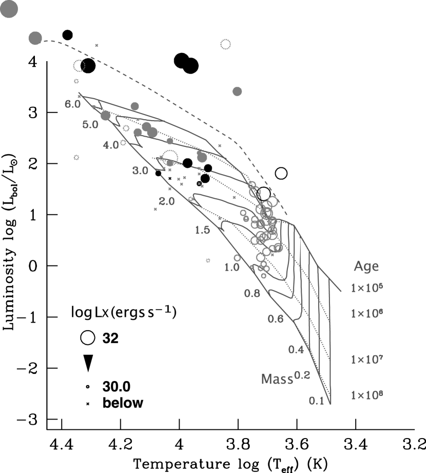
Figure 16: X-ray luminosity of young intermediate-mass stars in the HR diagram. Circle size is proportional to (log L_X ergs s^-1 $-$ 30) and crosses are log L_X $<$30 ergs s^-1 (both detected and upper limit sources). Luminosity upper limit on log L_X $\geq$30 ergs s^-1 is drawn by dotted circles. Black and grey are ASCA and ROSAT samples, respectively. HAeBes are drawn by filled circles and proto-HAeBe candidates (EC 95 and SVS 63E+W) are two black open circles. Grey open circles and crosses below log T${}_{\rm eff}\sim$3.8 K are sources in the Orion cloud (Gagné et al., 1995) (Undetected sources with upper limit above 10³⁰ ergs s^-1 are not included). The diagram is overlaid on a stellar evolutional track modeled by Palla & Stahler (1993). A broken line means the birth line when accretion rate is $\dot{M}$ = 10^-4 M_⊙ yr^-1.

L_X does not have clear correlation with N_H. We thus make a bubble chart of L_X in the HR diagram (Figure 16). Sources in the upper right region in the diagram have log L_X $\sim$32 ergs s^-1 and gradually decrease as they come close to the MS branch. A notable feature is the presence of an X-ray inactive region in the HR diagram: 3.8 $<$ log T_eff (K) $<$ 4.1 and 1.3 $<$ log L_bol (L_⊙) $<$ 1.9, which corresponds to the age older than 10⁶-year-old. Almost no source in this region has log L_X (ergs s^-1) $>$30. This X-ray inactive region may indicate that X-ray activity of HAeBes terminates after the age of $\sim 10^{6}$-year-old. Damiani et al. (1994) found a correlation between L_X and spectral type or L_bol, but Zinnecker & Preibisch (1994) did not. We now see that this difference is simply due to selection effects. Damiani et al. (1994) collected HAeBe samples close to the MS so that they found a similar X-ray characteristics to MS stars. Zinnecker & Preibisch (1994) examined young A-type samples such as V380 Ori and HR 5999. Their X-ray luminosity is comparable to early B-type stars and thus has no dependence on stellar spectral type.

The above discussion suggests that the X-ray activity decays with age and falls below log L_X (ergs s^-1) $\sim$30 at $\sim$10⁶-years-old. This age coincides with the end phase of outflow activity (Fuente et al., 1998). We therefore hypothesize that X-ray activity of HAeBes is triggered by reconnection of magnetic fields linking a star and its circumstellar disk (a star and disk dynamo activity) as it was claimed for the X-ray emission mechanism of low-mass protostars (e.g. Koyama et al., 1996; Hayashi et al., 1996; Montmerle et al., 2000). This model reconciles the lack of a magnetic dynamo on the stellar surface of HAeBes. To test the hypothesis, we correlate L_X of HAeBes with outflow activity by referring to tables in Maheswar et al. (2002) and Lorenzetti et al. (1999) and several individual papers (Table 10). Then, sources with log L_X $>$30 ergs s^-1 tend to have outflow activity, which might suggest a link between X-ray and outflow activity. Identification of outflow sources especially in crowded regions (e.g. EC 95, R CrA, T CrA) seems to have uncertainty, while the outflow from HD 200775 could be made by stellar winds (Fuente et al., 1998). More careful study would be required.

Our results suggest that X-ray emission from young HAeBes originates in magnetic activity. This means that magnetic activity plays an important role for both low-mass and intermediate-mass PMSs. We here propose a unified scenario for the X-ray activity of PMSs. In this scenario, stellar X-ray emission begins in the protostar phase when stars are deeply embedded in molecular cloud cores. In this phase, stars possess fossil magnetic fields from their parent clouds and exhibit violent magnetic activity linking a star and its disk, showing occasional X-ray flares. A part of the infalling gases goes out from the system with large amounts of angular momentum, which is later seen as molecular outflows or optical jets. After the star-disk dynamo activity disappears in $\sim$10⁶-year-old, low-mass stars still continue magnetic activity similar to a solar type dynamo. Stars between A - F5 lack any mechanism to produce hot plasma. X-ray activity ends for these stars, and the X-ray inactive region is seen in the HR diagram.

6 Relation of X-ray Activity to MS OB Stars

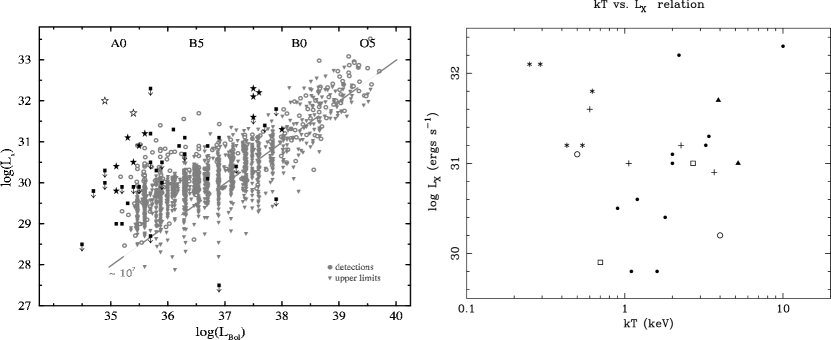
Figure 17: a: Log L_X $vs.$ log L_bol relation of HAeBes (black) overlaid on those of MSs (gray, figure 4 in Berghöfer et al. (1997)) (left panel). Marks of HAeBes are the same as those in Figure 13a. b: Log L_X $vs.$ kT relation of massive MS stars and HAeBes (right panel). Asterisks are cool components of 2T sources or 1T sources of massive MS stars. Crosses are hard X-ray tails of massive MS stars. Other marks for HAeBes and proto-HAeBes are the same as in Figure 15.

Figure 16 does not show any clear decrease of X-ray activity on B-type stars (log T${}_{eff}\gtrsim$ 4 (K)), but the L_X-L_bol ratio of Herbig Be stars is larger than MS B-type stars (see Figure 13b), which suggests some transition of X-ray activity close to the MS stage. We superimpose our HAeBe data on the L_X-L_bol graph of OB stars in the sky using ROSAT all-sky survey data (Figure 17a, the relation of OB stars referred to Berghöfer et al., 1997). Then, most of the HAeBe samples are above the higher end of OB MS stars. This would mean some transition of X-ray activity between HAeBe and MS phases. B-type stars are not generally thought to have accretion disks. The result may strengthen the star-disk dynamo hypothesis. On the other hand, we do not see any clear gap between MS and HAeBe plots. Berghöfer et al. (1997) suggests that the L_X/L_bol relation of early-type stars (log L_X/L_bol $\sim-$7), which is characteristic of a stellar wind origin, scatters later than B1$-$1.5 stars. This might imply that X-ray activity of HAeBes holds in the early stage of MS B-type stars.

Though no relation to the stellar evolution is claimed between O stars and HAeBes, comparison of their X-ray properties may help to understand X-ray activity. We thus made a kT and L_X graph (Figure 17b) of both types of stars (O stars$-$ $\delta$ Ori, $\lambda$ Ori; Corcoran et al. 1994: $\tau$ Sco; Cohen et al. 1997: $\zeta$ Oph, $\zeta$ Ori; Kitamoto et al. 2000). L_X for O stars are calculated from E.M. and kT from their references, using XSPEC 9.0. Some O stars have hard X-ray tail (e.g. Corcoran et al., 1993; Kitamoto & Mukai, 1996), which is separately shown in the figure. The hard tail component seems to share the region with HAeBe X-rays, while soft X-rays from O stars do not. Our results may suggest that the hard X-ray tail and HAeBe X-ray activity have something in common (e.g. high energy activity of fossil magnetic fields) though samples are quite limited.

7 Conclusion

X-ray emission from HAeBes has long been a puzzle. This is partly because the proper X-ray emission mechanism is not known for these intermediate-mass young stars and partly because satisfying observing results have not been obtained. By combining our ASCA analyses with previous ROSAT result, we find that the X-ray emission from HAeBes may originate in magnetic activity, which begins in the earliest phase of stars and continues to the MS stage. We list the results and implications below.

1. In the analyses of the ASCA data, 11 X-ray counterparts are detected. The X-ray luminosity ranges between log L_X = 30 – 32 ergs s^-1, which is significantly larger than the typical luminosity of low-mass stars.

2. Four (or five if we include TYHD) sources of the 11 detected sources (36$-$45%) exhibited time variation. Three HAeBes showed prominent variations with longer decay time scale (10$-$60 ksec).

3. X-ray spectra are reproduced by absorbed one or two temperature thin-thermal (MeKaL) models. The plasma temperature ranges between kT $\sim$1$-$5 keV, which is significantly higher than those of MS OB stars (kT $<$1 keV).

4. HAeBes have similar characteristics to low-mass YSOs in plasma temperature and time variability, but not in the L_X/L_bol ratio and $v_{rot}$ sin $i$ dependence. X-ray emission might originate from magnetic activity, but the activity might not be produced by solar-type magnetic dynamo.

5. If N_H is an indicator of stellar age, younger HAeBes tend to have hotter plasma. While L_X goes down below 10³⁰ ergs s^-1 after the stellar age of $\sim$10⁶-year-old. We propose that X-ray activity of HAeBes might be driven by magnetic interaction of a fossil field between the star and its accretion disk.

For statistical analyses of young intermediate and high-mass stars, Chandra will provide sophisticated data with little source contamination. Time profiles with high photon statistics can be obtained by XMM-Newton. While the micro-calorimeter onboard Astro-E2 will provide a powerful tool for performing high resolution spectroscopy in the hard X-rays above 2 keV.

Table 1: Stellar Parameters

Object	R.A. (2000)			Dec. (2000)			$d$	Sp. T	log Teff	log Lbol	AV	$v_{wind}$	$v_{rot}$ sin $i$
	(h	m	s)	(∘	′	′′)	(pc)		(K)	(L⊙)		(km s-1)	(km s-1)
BD +30 549	3	29	19.8	31	24	57	350	B8	4.08	1.1	1.9	$\cdots$	$\cdots$
V892 Tau	4	18	40.6	28	19	17	160	A6	$\cdots$	$\cdots$	4.1	250	$\cdots$
AB Aur	4	55	45.8	30	33	4	144	A0	3.98	1.7	0.5	260	140
V372 Ori	5	34	47.0	$-$5	34	15	460	B9.5+A0.5	3.93	2.2	0.5	$\cdots$	125
HD 36939	5	34	55.3	$-$5	30	22	460	B8–9	4.05	1.9	0.5	$\cdots$	275
HD 245185	5	35	9.6	10	1	52	400	A2	3.96	1.3	0.1	$\cdots$	150
LP Ori	5	35	9.8	$-$5	27	53	460	B2	4.29	3.1	0.7	$\cdots$	100
MR Ori	5	35	17.0	$-$5	21	46	460	A2	3.93	1.9	1.6	$\cdots$	$\cdots$
V361 Ori	5	35	31.4	$-$5	25	16	460	B1.5 or B4	4.14	2.6	0.4	$\cdots$	50
T Ori	5	35	50.0	$-$5	28	42	460	A3	3.93	1.6	1.1	$\cdots$	100
V380 Ori	5	36	25.4	$-$6	42	58	460	B9–A0	3.97	1.9	1.4	260	200
BF Ori	5	37	13.3	$-$6	35	1	430	A5–6	3.90	0.1	0.3	$\cdots$	100
MWC 120	5	41	2.3	$-$2	43	1	500	A2	3.95	1.3	0.03	$\cdots$	120
VY Mon	6	31	7.0	10	26	5	800	O9$-$B8	4.05	2.9	7.4	$\cdots$	$\cdots$
VY Mon G2	6	31	8.2	10	26	1	800	A0	(3.99)	4.0	1.6	$\cdots$	$\cdots$
V590 Mon	6	40	41.3	9	48	1	800	B7	4.09	2.6	0.6	$\cdots$	$\cdots$
LkH$\alpha$ 218	7	2	42.3	$-$11	26	10	1150	B9	4.03	2.1	1.5	$\cdots$	$\cdots$
Z CMa	7	3	43.2	$-$11	33	6	1150	F6	3.80	3.4	2.8	$\cdots$	$<$130
LkH$\alpha$ 220	7	4	5.4	$-$11	26	0	1150	B5	4.19	2.4	$\cdots$	$\cdots$	$\cdots$
HD 76534	8	55	8.7	$-$43	28	0	830	B2	4.34	3.9	1.2	$\cdots$	110
HD 97048	11	8	3.3	$-$77	39	17	180	B9–A0	4.00	1.6	1.2	$\cdots$	140
HD 97300	11	9	50.0	$-$76	36	48	188	B9	(4.03)	1.5	1.3	$\cdots$	$\cdots$
HD 104237	12	0	5.1	$-$78	11	35	116	A4	3.93	1.6	0.3	500	$\cdots$
IRAS 12496$-$7650	12	53	16.1	$-$77	7	2	200	A–F	(3.91)	1.7	12	$\cdots$	$\cdots$
HR 5999	16	8	34.3	$-$39	6	18	210	A5–7	3.90	1.9	0.5	100	180
HD 147889	16	25	24.3	$-$24	27	57	140	B2	4.34	3.3	3.3	$\cdots$	$\cdots$
Hen 3$-$1191	16	27	14.2	$-$48	39	28	$\cdots$	B0	$\cdots$	$\cdots$	$\cdots$	$\cdots$	$\cdots$
V921 Sco	16	59	6.9	$-$42	42	8	500	B4–5	(4.14)	3.0	7.1	500	$\cdots$
MWC 297	18	27	39.6	$-$3	49	52	250	B1.5	(4.38)	4.5	8	380	350
HD 176386	19	1	38.9	$-$36	53	27	122	B9	4.03	1.7	0.6	$\cdots$	$\cdots$
TY CrA	19	1	40.8	$-$36	52	34	130	B7–9	(4.07)	1.8	1.0	$\cdots$	10
R CrA	19	1	53.7	$-$36	57	8	130	B8	(4.06)	2.1	1.9	$\cdots$	$\cdots$
T CrA	19	1	59.0	$-$36	58	0	130	F0	(3.86)	0.9	1.7	$\cdots$	40
HD 200775	21	1	36.9	68	9	48	429	B2.5	4.31	3.9	1.9	280	60
MWC 1080	23	17	26.1	60	50	43	2200	A0–3	(3.96)	3.9	4.4	400	200
EC 95	18	29	57.9	1	12	47	310	K0–K4	(3.65)	1.8	36	$\cdots$	$\cdots$

Note. — Sp.T: spectral type, T_eff: parentheses show average temperature of their spectral type. References$-$ van den Ancker et al. (1997, 1998), Thé et al. (1994), Preibisch (1998), Nisini et al. (1995), Benedettini et al. (1998), Grady et al. (1993), Böhm & Catala (1995), Drew et al. (1997), Casey et al. (1998), van den Ancker et al. (1998), Corporon & Lagrange (1999).

Table 2: ASCA Observation Log

Seq. ID	Abbrevation	Date	Ontime	SIS Mode	Exposure
					SIS	GIS
			(ksec)		(ksec)	(ksec)
23021000	SVS13	1995 Aug 30	211.0	$\cdots$	$\cdots$	93.0
23009000	IC359	1995 Sep 2	104.6	4F/B LD 0.55	27.4	37.8
23042000	SU Aur	1995 Feb 25	114.5	2F/B	40.8	45.0
20004000	Ori Trap1	1993 Aug 30	51.4	4F/B	19.3	18.0
21005000	L1641N	1994 Mar 13	97.5	$\cdots$	$\cdots$	34.6
21025000	Lamb Ori	1994 Mar 12	51.3	2/1F	21.8	22.4
23019000	Ori OB1	1995 Oct 4	79.8	$\cdots$	$\cdots$	28.6
26007000	PSRJ0631	1998 Oct 16	157.2	$\cdots$	$\cdots$	81.6
25015000	15 Mon	1997 Oct 18	96.9	1F LD 0.48	36.6	36.1
23014000	Z CMa	1995 Mar 31	79.6	1F	30.5	37.6
55030000	Vela Shrap	1997 May 9	39.6	$\cdots$	$\cdots$	12.3
21009000	ChamI I	1994 May 14	39.3	4F/B	8.5	15.2
27017000	ChamI V	1999 Aug 7	258.9	2F	82.4	75.0
23003000	HD104237	1995 Apr 3	67.6	1F	29.9	27.1
24000000	ChamII	1996 Mar 10	69.1	$\cdots$	$\cdots$	24.9
24008000	Lupus3	1996 Feb 22	97.6	4F/B LD 0.7	18.2	41.3
20015010	Rho-Oph	1993 Aug 20	73.6	$\cdots$	$\cdots$	41.1
55003060	Gal R 1	1997 Sep 3	31.9	$\cdots$	$\cdots$	9.7
54004020	Gal R 2	1996 Aug 31	27.6	4F/B	12.2	11.8
21007000	MWC297 1	1994 Apr 8	49.9	1F	10.5	10.3
21007010	MWC297 2	1994 Apr 12	24.9	1F	5.3	5.0
21007020	MWC297 3	1994 Apr 12	45.4	1F	12.9	12.3
21001000	R CrA 1	1994 Apr 4	90.3	4F/B	38.4	39.4
21002000	R CrA 2	1994 Apr 8	97.5	4F/B	35.5	36.9
24016000	R CrA 3	1996 Apr 5	160.2	1F	65.2	48.8
24016010	R CrA 4	1996 Oct 18	30.8	1F	10.6	11.7
66017000	R CrA 5	1998 Apr 19	57.6	1F	17.1	16.2
26018000	R CrA 6	1998 Oct 19	108.3	1F	31.5	34.1
23029000	HD200775	1995 Nov 17	110.0	1F LD 0.55	46.0	48.7
21006000	MWC1080	1993 Dec 8	86.0	1F	36.1	38.4
25021000	Serp	1997 Apr 13	246.2	4F LD 0.7	87.4	89.9

Note. — Ontime: duration of observations, SIS Mode: number of CCD chips working (4/2/1), Data Format (Faint/Bright), Level Discri (Unit keV), Left values on slashes are CCD modes during the high telemetry mode and right values are modes during the medium and low telemetry modes.

Table 3: ROSAT Data Log

Object	Obs ID	Date	Exp.	Detector	Usage
			(ksec)
HD 245185	RH202047N00	1995 Mar 16	9.4	HRI	U
BF Ori	RH900010A01	1992 Mar 14	4.8	HRI	U
MWC 120	RP900189N00	1991 Sep 19	24.2	PSPC	U
VY Mon	RP900355N00	1992 Oct 6	5.6	PSPC	ID
	RP900355A01	1993 Mar 14	4.6	PSPC	ID
	RP900355A02	1993 Sep 16	5.4	PSPC	ID
	RP900355A03	1994 Mar 29	5.1	PSPC	ID
V590 Mon	RH200130A00	1991 Mar 20	19.6	HRI	U
LkH$\alpha$ 218	RP201011N00	1993 Apr 22	19.7	PSPC	U
LkH$\alpha$ 220	RH202153N00	1996 Apr 6	33.5	HRI	U
MWC 297	RH202048N00	1995 Sep 28	1.1	HRI	ID
HD 200775	RH202319N00	1997 Aug 11	4.8	HRI	ID

Note. — U: used for upper limit measurement (See also Table 6). ID: used for source identification.

Table 4: Selected Regions

Object	Det.	Region
		Source	Background
V892 Tau	S	c(3)	sym V1023 Tau
V380 Ori	G	c(3)	a(3/6)
VY Mon	G	e(4.5/2.5)	$sf$ (sym optical axis)
HD 104237	S	c(2.5)	whole chip excluding $sr$
	G	c(3)	a(3/6)
IRAS 12496$-$7650	G	c(3)	a(3/6)
HR 5999	S	e(0.66/0.25)	sym HR 6000
V921 Sco	G	c(3)	a(3/6)
MWC 297	S	c(3)	a(3/4.4)
	G	c(3)	a(3/6)
TY CrA	S	e(0.74/0.53)	sym HD 176386
HD 176386	S	e(0.64/0.42)	sym TY CrA
TYHD	G	c(2.5)	sym the R CrA protostar cluster
HD 200775	S	c(2.5)	$sf$
	G	c(3)	sym the SE source
MWC 1080	S	c(2.5)	$sf$
	G	c(3)	a(3/6)
EC 95	S	c(3)	b(9/3)
	G	c(3)	a(3/6)

Note. — c($num$): $num$ arcmin radius circle centered on a target, e($num1$/$num2$): ellipse with $num1$ arcmin long and $num2$ arcmin short axes, a($num1$/$num2$): annular circle with $num1$ arcmin inner and $num2$ arcmin outer radii, b($num1$/$num2$): $num1$ arcmin $\times$ $num2$ arcmin box, sym $sth$: symmetrical region with respect to $sth$, $sr$: source region, $sf$: source free region

Table 5: ASCA Detected Sources

Object	Obs. ID	Detected Position								Net Count
		R.A. (2000)			Dec. (2000)			Det.		SIS		GIS		Total
		(h	m	s)	(∘	′	′′)			(cnts)	(%)	(cnts)	(%)	(cnts)
V892 Tau	IC359	4	18	39.8	28	19	16	S		722	(59)	$\cdots$	( $\cdots$ )	722
V380 Ori	L1641N	5	36	23.8	$-$6	43	18	G2		$\cdots$	( $\cdots$ )	109	(33)	109
VY Mon (/G2)	PSRJ0631	6	31	3.1	10	26	46	G		$\cdots$	( $\cdots$ )	338	(36)	338
HD 104237	HD104237	12	0	6.2	$-$78	11	29	S		2427	(84)	916	(74)	3343
IRAS 12496$-$7650	ChamII	12	53	16.5	$-$77	7	6	G		$\cdots$	( $\cdots$ )	100	(31)	100
HR 5999	Lupus3	16	8	34.9	$-$39	6	12	S		143	(48)	$\cdots$	( $\cdots$ )	143
V921 Sco	Gal R 2	16	59	8.7	$-$42	42	30	G		$\cdots$	( $\cdots$ )	151	(38)	151
MWC 297	MWC297 1	18	27	37.9	$-$3	49	36	S		353	(62)	257	(67)	610
	MWC297 2									1023	(79)	904	(87)	1927
	MWC297 3									528	(64)	349	(70)	877
TY CrA	R CrA 1	19	1	40.8	$-$36	52	31	S		524	(67)	$\cdots$	( $\cdots$ )	524
	R CrA 4									75	(56)	$\cdots$	( $\cdots$ )	75
	R CrA 6									437	(71)	$\cdots$	( $\cdots$ )	437
HD 176386	R CrA 1	19	1	38.7	$-$36	53	18	S		227	(49)	$\cdots$	( $\cdots$ )	227
	R CrA 4									45	(52)	$\cdots$	( $\cdots$ )	45
	R CrA 6									228	(49)	$\cdots$	( $\cdots$ )	228
TYHD	R CrA 1									$\cdots$	( $\cdots$ )	1488	(78)	1488
	R CrA 2									$\cdots$	( $\cdots$ )	676	(64)	676
	R CrA 3									$\cdots$	( $\cdots$ )	1585	(78)	1585
	R CrA 4									$\cdots$	( $\cdots$ )	510	(73)	510
	R CrA 5									$\cdots$	( $\cdots$ )	543	(91)	543
	R CrA 6									$\cdots$	( $\cdots$ )	1029	(68)	1029
HD 200775	HD200775	21	1	34.9	68	10	1	S		3361	(85)	1641	(69)	5002
MWC 1080	MWC1080	23	17	24.0	60	50	43	S		273	(33)	185	(27)	458
EC 95	Serp	18	29	58.3	1	12	43	S		3216	(75)	3679	(70)	6895

Note. — Det.: detectors measuring source positions (S: SIS, G: GIS), Net Count: background subtracted source counts, Parentheses: source event ratio defined as “source counts / (source + background) counts”, Total: net counts of SIS + GIS, TYHD: GIS data merged with TY CrA and HD 176386.

Table 6: ASCA Non-detected Sources

Object	ASCA							ROSAT
	Obs. ID	Flux upper limit		Det.	Log LX	Note		Ref.	Flux		Log LX	Note	Log $\frac{L_{X}}{L_{bol}}$
		Photon	Energy						Photon	Energy
BD +30 549	SVS13	2.1 10-2	1.1 10-12	G	$<$31.2	con.		1	$\cdots$	$\cdots$	$<$29.8	$\cdots$	$<-$4.9
AB Aur	SU Aur	3.1 10-2	7.4 10-13	S	$<$30.3	con.		2	$\cdots$	$\cdots$	29.5	$\cdots$	$-$5.7
V372 Ori	Ori Trap1	3.5 10-2	1.3 10-12	G	$<$31.5	$\cdots$		3	$\cdots$	$\cdots$	30.3	$\cdots$	$-$5.5
HD 36939	Ori Trap1	4.6 10-2	1.7 10-12	G	$<$31.6	$\cdots$		3	$\cdots$	$\cdots$	$<$29.9	$\cdots$	$<-$5.6
HD 245185	Lamb Ori	1.6 10-2	3.3 10-13	S	$<$30.8	$\cdots$		4	$<$2.4 10-3	$<$9.7 10-14	$<$30.3	$\cdots$	$<-$4.6
LP Ori	Ori Trap1	3.6 10-1	9.2 10-12	S	$<$32.4	con.		3	$\cdots$	$\cdots$	30.1	$\cdots$	$-$6.6
MR Ori	Ori Trap1	2.7	9.4 10-11	S	$<$33.4	con.		3	$\cdots$	$\cdots$	$<$29.9	$\cdots$	$<-$5.2
V361 Ori	Ori Trap1	9.8 10-1	2.3 10-11	S	$<$32.8	con.		3	$\cdots$	$\cdots$	30.9	$\cdots$	$-$5.4
T Ori	Ori Trap1	6.5 10-2	1.6 10-12	S	$<$31.6	con.		3	$\cdots$	$\cdots$	29.9	$\cdots$	$-$5.3
BF Ori	L1641N	$\cdots$	5.8 10-13	G	$<$31.1	ano.		4	$<$2.2 10-3	$<$6.7 10-14	$<$30.2	$\cdots$	$<-$3.5
MWC 120	Ori OB1	9.5 10-3	3.1 10-13	G	$<$31.0	$\cdots$		4	$<$2.7 10-3	$<$3.3 10-14	$<$30.0	$\cdots$	$<-$4.9
V590 Mon	15 Mon	4.8 10-2	1.2 10-12	S	$<$32.0	$\cdots$		4	4.2 10-3	2.4 10-13	31.3	$\cdots$	$-$4.8
LkH$\alpha$ 218	Z CMa	9.9 10-2	4.4 10-12	G	$<$32.8	$\cdots$		4	$<$3.7 10-2	$<$1.2 10-12	$<$32.3	con.	$<-$3.4
Z CMa	Z CMa	1.9 10-2	8.9 10-13	S	$<$32.1	$\cdots$		2	$\cdots$	$\cdots$	31.1	$\cdots$	$-$5.8
LkH$\alpha$ 220	Z CMa	8.5 10-3	2.8 10-13†	G	$<$31.6	con.		4	$<$7.0 10-4	$<$2.2 10-14	$<$30.5	$\cdots$	$<-$5.4
HD 76534	Vela Shrap	1.0 10-2	4.3 10-13	G	$<$31.6	$\cdots$		5	$\cdots$	$\cdots$	$\cdots$	$\cdots$	$<-$5.9
HD 97048	ChamI V	$\cdots$	1.8 10-13	S	$<$29.8	ano.		2	$\cdots$	$\cdots$	29.0	$\cdots$	$-$6.2
HD 97300	ChamI I	5.1 10-2	2.3 10-12	G	$<$31.0	con.		6	$\cdots$	$\cdots$	29.0	$\cdots$	$-$6.1
HD 147889	Rho-Oph	$\cdots$	1.7 10-12	G	$<$30.6	ano.		7	$\cdots$	$\cdots$	$<$27.5	$\cdots$	$<-$9.4
Hen 3-1191	Gal R 1	2.3 10-2	7.5 10-13†	G	$\cdots$	$\cdots$		5	$\cdots$	$\cdots$	$\cdots$	$\cdots$	$\cdots$
R CrA	R CrA 1	1.4 10-1	5.2 10-12	S	$<$31.0	con.		2	$\cdots$	$\cdots$	$<$28.7	$\cdots$	$<-$7.0
T CrA	R CrA 1	4.0 10-2	1.5 10-12	S	$<$30.5	con.		2	$\cdots$	$\cdots$	$<$28.5	$\cdots$	$<-$6.0

Note. — The column of ASCA, flux upper limit (0.5–10 keV), Photon [cnts s^-1 ]: 3$\sigma$ level or count rate of source contamination estimated from a 40^′′ and 80^′′ square regions for the SIS and GIS, respectively. Energy [ergs cm^-2 s^-1 ]: unabsorbed energy flux upperlimit calculated using the PIMMS package, assuming thin-thermal plasma with kT $\sim$2 keV and N_H converted from the A_V, Log L_X [ergs s^-1 ] (0.5–10 keV): absorption corrected X-ray luminosity, Det.: detectors measuring count rates (S: SIS, G: GIS), Sources marked as “con.” have source contamination, Sources marked as “ano.” are identified as the other objects. ^† assuming no absorption (N_H = 0.0 cm^-2). The column of ROSAT, ref.: reference of log L_X, 1: Preibisch (1997), 2: Zinnecker & Preibisch (1994), 3: Gagné et al. (1995), 4: this work, 5: no pointing observation, 6: Feigelson et al. (1993), 7: Casanova et al. (1995), Flux (0.1–2.4 keV): Photon [cnts s^-1 ], Energy [ergs cm^-2 s^-1 ], absorption corrected energy flux assuming thin-thermal plasma of kT $\sim$2 keV and N_H converted from A_V, Log L_X [ergs s^-1 ] (0.1–2.4 keV): absorption corrected X-ray luminosity. Sources marked as “con.” have source contamination.

Table 7: Result of ASCA Timing Analysis

Object	St.	Det.	Bin	Constant Fittings
				Mean	Reduced $\chi^{2}(d.o.f)$		Var.
			(sec)	(cnts s-1)
V892 Tau		S	2048	1.5 10-2	1.42	(27)	n
V380 Ori		G2	2048	2.4 10-3	0.94	(33)	n
VY Mon (/G2)		G	2048	8.9 10-3	1.69	(70)	y
HD 104237		SG	2048	2.8 10-2	2.62	(31)	y
IRAS 12496$-$7650		G	2048	1.6 10-3	1.00	(30)	n
HR 5999		S	2048	3.4 10-3	1.08	(21)	n
V921 Sco		G	2048	6.3 10-3	0.51	(11)	n
MWC 297	1	SG	2048	1.5 10-2	0.25	(10)	n
	2	SG	2048	9.0 10-2	4.51	(7)	y
	3	SG	2048	1.6 10-2	4.56	(13)	y
TY CrA	1	S	2048	6.4 10-3	0.79	(34)	n
	4	S	2048	5.8 10-3	1.09	(12)	n
	6	S	2048	6.7 10-3	0.90	(39)	n
HD 176386	1	S	2048	2.8 10-3	0.83	(33)	n
	4	S	2048	4.4 10-3	0.40	(12)	n
	6	S	2048	2.1 10-3	1.21	(39)	n
TYHD	1	G	2048	1.4 10-2	1.67	(36)	y
	2	G	2048	1.3 10-2	1.42	(37)	n
	3	G	4096	4.0 10-2	3.14	(33)	y
	4	G	2048	1.5 10-2	1.79	(14)	n
	5	G	2048	1.8 10-2	0.84	(21)	n
	6	G	2048	6.7 10-3	0.90	(39)	n
HD 200775		S1G	2048	2.1 10-2	1.71	(47)	y
MWC 1080		SG	4096	3.0 10-3	0.79	(19)	n
EC 95		SG	2048	1.7 10-2	2.28	(92)	y

Note. — St.: number of observation ID., Det.: detector (S: SIS, G: GIS, SG: SIS + GIS), Bin.: binning time scales of light curves, Mean: average count rates derived from constant fittings, Var.: sources showing time variation above 96% confidence level, TYHD: GIS data merged with TY CrA and HD 176386.

Table 8: Result of ASCA Spectral Analysis

Object	St.	Det.	Model	kT		$E.M.$		NH		Reduced $\chi^{2}(d.o.f.)$		Flux	LX	LX/Lbol
V892 Tau		S	1T	2.0	(1.6–2.5)	54.0	(53.9–54.1)	1.2	(0.9–1.6)	0.99	(51)	1.22	$\cdots$	$\cdots$
		S	2T	2.0	(fix)	54.0	(fix)	1.8	(fix)	0.87	(54)	1.02	31.0	–4.4
				0.5	(0.3–0.7)	54.3	(53.9–55.4)	1.7	(1.2–2.8)	$\cdots$		0.20	31.3	$\cdots$
V380 Ori		G2	1T	3.2	(0.7–11.0)	54.1	(53.9–54.3)	0.0	(0.0–1.5)	1.31	(14)	0.59	31.2	–4.4
		G2	1TF	2.4	(1.3–6.1)	54.2	(54.0–54.4)	0.3	(fix)	1.25	(15)	0.68	31.2	–4.3
VY Mon (/G2)	LS	G	1T	2.9	(2.0–4.6)	55.1	(55.0–55.3)	0.6	(0.2–1.0)	1.40	(42)	1.21	32.2	–5.4
	LS	G	1TG	2.2	(1.6–3.3)	55.2	(55.0–55.4)	0.8	(0.4–1.2)	1.23	(40)	1.18	32.2	–5.4
	HS	G	1T	6.0	(3.8–12.3)	55.2	(55.1–55.3)	0.4	(0.1–0.8)	1.29	(45)	2.49	32.4	–4.1
	HS	G	1TLS	20.3	(3.0–)	54.8	(54.7–55.2)	0.6	(0.0–2.5)	1.28	(45)	1.24	32.1	–4.4
HD 104237		SG	1T	2.1	( $\cdots$ )	53.3	( $\cdots$ )	0.0	( $\cdots$ )	3.82	(89)	$\cdots$	$\cdots$	$\cdots$
		SG	2T	0.7	(0.6–0.7)	52.9	(52.8–53.1)	0.1	(0.0–0.2)	1.57	(87)	0.43	29.9	–5.2
				4.0	(3.3–4.8)	53.1	(53.0–53.1)	0.1	(com.)	$\cdots$		0.93	30.2	–4.9
IRAS 12496$-$7650		G	1T	2.0	(0.9–7.2)	54.1	(53.4–55.3)	13	(6.2–24)	0.93	(14)	0.29	31.1	–4.2
HR 5999		S	1T	0.9	(0.6–1.7)	53.9	(53.5–54.3)	0.7	(0.0–1.2)	1.15	(11)	0.37	30.9	–4.6
		S	1TF	1.6	(1.2–2.4)	53.5	(53.4–53.6)	0.1	(fix)	1.27	(12)	0.44	30.4	–5.1
V921 Sco		G	1T	2.8	(1.1–9.1)	55.0	(54.6–56.1)	4.9	(2.3–14)	0.96	(18)	1.14	32.1	–4.5
MWC 297	1	SG	1T	3.4	(2.4–5.1)	54.2	(54.1–54.4)	2.4	(1.8–3.1)	0.92	(43)	1.18	31.3	–6.8
	2	SG	1T	6.5	(4.7–9.6)	54.9	(54.8–55.0)	2.5	(2.1–2.8)	1.04	(105)	9.23	32.1	–6.0
	3	SG	1T	3.4	(2.6–4.8)	54.2	(54.1–54.3)	1.9	(1.5–2.4)	0.89	(63)	1.31	31.3	–6.7
TY CrA	1	S	1T	1.8	(0.8–2.3)	53.4	(53.3–53.5)	0.3	(0.1–0.5)	1.02	(28)	0.76	30.4	–5.1
	4	S	1TF	1.8	(1.2–3.4)	53.5	(53.3–53.7)	0.4	(fix)	1.33	(5)	0.89	30.5	–4.9
	6	S	1T	1.2	(1.0–1.4)	53.7	(53.5–53.8)	0.6	(0.3–0.9)	0.87	(25)	0.82	30.6	–4.8
HD 176386	1	S	1T	1.3	(1.0–1.8)	52.8	(52.7–52.9)	0.0	(0.0–0.2)	0.90	(16)	0.32	29.8	–5.5
	4	S	1TF	1.0	(0.7–1.5)	53.0	(52.8–53.2)	0.0	(fix)	0.56	(4)	0.50	30.0	–5.3
	6	S	1T	1.9	(1.3–2.8)	52.9	(52.8–53.9)	0.0	(0.0–0.2)	1.93	(13)	0.39	29.8	–5.4
TYHD	1	G	1T	2.1	(1.9–2.4)	53.6	(53.6–53.6)	0.0	(0.0–0.1)	1.87	(26)	1.86	$\cdots$	$\cdots$
	2	G	1T	1.7	(1.2–2.0)	53.6	(53.6–53.8)	0.0	(0.0–0.5)	0.66	(41)	1.74	$\cdots$	$\cdots$
	3LS	G3	1T	2.6	(2.1–3.1)	53.7	(53.6–53.7)	0.0	(0.0–0.1)	0.79	(65)	2.43	$\cdots$	$\cdots$
	3HS	G3	1T	3.0	(2.4–3.8)	53.8	(53.8–53.9)	0.0	(0.0–0.2)	0.88	(22)	3.87	$\cdots$	$\cdots$
	4	G	1T	2.5	(2.0–3.3)	53.6	(53.5–53.6)	0.0	(0.0–0.2)	1.18	(30)	1.92	$\cdots$	$\cdots$
	5	G	1T	2.1	(1.3–2.6)	53.7	(53.6–53.9)	0.0	(0.0–0.4)	0.98	(25)	2.26	$\cdots$	$\cdots$
	6	G	1T	1.7	(1.4–1.9)	53.5	(53.5–53.6)	0.0	(0.0–0.2)	1.03	(64)	1.49	$\cdots$	$\cdots$
HD 200775		SG	1T	1.7	(1.6–1.9)	54.5	(54.5–54.6)	0.1	(0.0–0.2)	1.39	(211)	1.11	31.5	–6.0
		SG	2T	0.5	(0.4–0.7)	55.2	(55.1–55.4)	0.9	(0.8–1.0)	1.15	(209)	0.59	32.1	–5.3
				2.8	(1.9–3.8)	54.2	(54.1–54.5)	0.9	(com.)	$\cdots$		0.47	31.3	–6.2
MWC 1080		SG	1T	10.0	(3.8–)	55.1	(55.0–55.3)	1.0	(0.3–2.2)	1.02	(56)	0.26	32.3	–5.1
		SG	1TGe	7.2	(3.0–)	55.1	(54.9–55.3)	1.0	(0.3–2.2)	0.97	(54)	0.27	32.3	–5.1
EC 95		SG	1T	3.9	(3.5–4.4)	54.5	(54.5–54.6)	2.3	(2.0–2.5)	1.20	(205)	1.97	31.7	–3.7

.

Note. — St.: number of observation ID and/or status (HS: high or flare state, LS: low or quiescent state), Det.: S: SIS, G: GIS, SG: SIS+GIS, Model: 1T: 1-temperature, 2T: 2-temperature, ^G/LS: adding the components of Gaussian/low state, ^F: fixing N_H value, kT [keV], E.M. [log, cm^-3], N_H [10²² cm^-2 ], com.: common N_H values with the above column, fix: parameter is fixed, Parentheses show 90% confidence level, Reduced $\chi^{2}$: parentheses denote number of degree of freedom ($d.o.f$), Flux [10^-12 ergs cm^-2 s^-1 ]: observed flux (0.5–10 keV), L_X [log, ergs s^-1 ]: absorption corrected X-ray luminosity between 0.5–10 keV, L_X/L_bol [log], TYHD: GIS data merged with TY CrA and HD 176386

Table 9: Fitting Results of the Flare Light Curves

Object	Obs. ID	Det.	Iqui	Ipeak	$\tau_{ris}$	$\tau_{dec}$
			(cnts s-1)	(cnts s-1)	(104 sec)	(104 sec)
MWC 297	MWC297 2,3	SG	2.3 (2.1–2.4) 10-2	$>$ 1.2 10-1	$\cdots$	5.6 (4.5–7.0)
VY Mon	PSRJ0631	G	2.5 (1.7–2.9) 10-3	$>$ 3.8 10-3	$\cdots$	3.6 (2.0–7.4)
TYHD	R CrA3	G	3.6 (3.4–3.8) 10-2	$\sim$ 7.5 10-2	$\sim$ 1	2.4 (1.3–8.0)

Note. — Det.: detector, S: SIS, G: GIS., $\tau_{dec}$: $e$-folding time fit by a constant and exponential decay model. $\tau_{ris}$: the period between the constant level to the flux peak.

Table 10: Outflow Activity

log LX	Outflow Activity
(ergs s-1)	Yes	No activity found
Above 30	V380 Ori1,2, Z CMa2, IRAS 12496-76503,5, HD 2007752,4, MWC 10802,6, EC 957,	V892 Tau2, HD 1042378, HR 59992, MWC2973
Below 30	R CrA2,3, T CrA2	T Ori2, HD 765342, HD 970483

Note. — References: ¹Corcoran & Ray (1995), ²Maheswar et al. (2002) (Table 2, column 8), ³Lorenzetti et al. (1999) (Table 2, column 5), ⁴Fuente et al. (1998), ⁵Hughes et al. (1989), ⁶Poetzel et al. (1992), ⁷Eiroa & Casali (1989), ⁸Knee & Prusti (1996). Sources with blanks in the columns of Maheswar et al. (2002) and Lorenzetti et al. (1999) are listed in ”no activity found”.

Figure 1: a: ASCA image of the V892 Tau field (12^′ $\times$12^′) (top left panel). The contour image smoothed with a Gaussian function of $\sigma\sim$2 pixel (SIS: 6.^′′4 pixel^-1, GIS: 14.^′′7 pixel^-1) is drawn by 0.4 cnts pixel^-1 for the SIS and 0.5 cnts pixel^-1 for the GIS. A dot-dash line represents 5$\sigma$ detection levels of the Poisson-distributed photon error of the background. Dash-lines are the detector rims. The filled circle on the bottom right shows the typical error circle of the SIS (20^′′) and the GIS (40^′′). The coordinate system is J2000. Legend $-$ star: HAeBe, diamond: infrared source, triangle: young star and PMS object, square: radio source, cross: normal star, asterisk: galaxy. The source category is referred to the SIMBAD database. b: SIS light curves of V892 Tau (top right panel). The background is subtracted. The vertical axis is averaged detector count rates. Dotted lines are the zero level. 1 bin is 2,048 sec. c: SIS spectrum of V892 Tau including the component of V410 X-ray 7 (2T model in Table 8, bottom left panel). The solid and dotted lines show the best-fit model of the total and each component, respectively. The residual of the best-fit model is displayed in the lower section.

Figure 2: a: GIS image of the V380 Ori field (left panel). See Figure 1a for details. b: GIS spectrum of V380 Ori (right panel). See Figure 1c for details.

Figure 5: a: GIS image of IRAS 12496$-$7650 (left panel). b: GIS spectrum of IRAS 12496$-$7650 (right panel).

Figure 7: a: GIS image of V921 Sco (left panel). b: GIS spectrum of V921 Sco (right panel).

Figure 11: a: SIS image of MWC 1080 (top left panel). The count rate per solid-line is 0.2 cnts pixel^-1. b: Light curves of MWC 1080 (top right panel). c: SIS spectrum of MWC 1080 (bottom left panel).

Figure 13: a: Log L_X $vs.$ log L_bol relation (top left panel), b: log L_X/L_bol $vs.$ log T_eff relation (top right panel), c: log L_X/L_bol $vs.$ $v_{rot}$ sin $i$ (bottom left panel). Filled and open stars represent HAeBes and proto-HAeBes of ASCA samples, respectively. Filled squares represent HAeBes of ROSAT samples. Points with arrows represent upper-limit. L_X of ROSAT is converted to the ASCA band assuming kT = 2 keV, abundance = 0.3Z_⊙ and N_H converted from A_V (Ryter, 1996). The plot in the upper left box represents typical error ranges of ROSAT samples if kT changes between 0.5–4 keV. Barred lines in the figure (a) show log L_X/L_bol = $-$3, $-$5 and $-$7 from the top, respectively.

Figure 14: kT $vs.$ terminal velocity of the stellar wind ($v_{wind}$). Dots are 1T sources. Open circles and squares are dominant (i.e. large L_X) and minor (i.e. small L_X) components of 2T sources, respectively. The solid line denotes the plasma temperature when whole kinetic energy converts to the thermal energy (i.e. 3$kT$=$m_{p}v_{wind}^{2}/2$, $m_{p}$: proton mass).

Figure 15: kT dependence on N_H. Dots, open circles and squares are the same as in Figure 14. Proto-HAeBes (1T) are shown as filled triangles. N_H less than 10²¹ cm^-2 is referred to the A_V-converted N_H.

References

- Benedettini et al. (1998) Benedettini, M., Nisini, B., Giannini, T., Lorenzetti, D., Tommasi, E., Saraceno, P., & Smith, H. A. 1998, A&A, 339, 159
- Berghöfer et al. (1997) Berghöfer, T. W., Schmitt, J. H. M. M., Danner, R., & Cassinelli, J. P. 1997, A&A, 322, 167
- Bertout et al. (1999) Bertout, C., Robichon, N., & Arenou, F. 1999, A&A, 352, 574
- Bibo et al. (1992) Bibo, E. A., Thé, P. S., & Dawanas, D. N. 1992, A&A, 260, 293
- Böhm & Catala (1995) Böhm, T., & Catala, C. 1995, A&A, 301, 155
- Böhm et al. (1996) Böhm, T., Catala, C., Donati, J. F., Welty, A., Baudrand, J., Butler, C. J., Carter, B., Collier-Cameron, A., Czarny, J., Foing, B., Ghosh, K., Hao, J., Houdebine, E., Huang, L., Jiang, S., Neff, J. E., Rees, D., Semel, M., Simon, T., Talavera, A., Zhai, D., & Zhao, F. 1996, A&AS, 120, 431
- Briceño et al. (1998) Briceño, C., Hartmann, L., Stauffer, J., & Martín, E. 1998, AJ, 115, 2074
- Brooke et al. (1993) Brooke, T. Y., Tokunaga, A. T., & Strom, S. E. 1993, AJ, 106, 656
- Burke et al. (1994) Burke, B. E., Mountain, R. W., Daniels, P. J., & Dolat, V. S. 1994, IEEE Trans. NS-41, 375
- Cantó et al. (1984) Cantó, J., Rodríguez, L. F., Calvet, N., & Levreault, R. M. 1984, ApJ, 282, 631
- Cardelli & Wallerstein (1989) Cardelli, J. A., & Wallerstein, G. 1989, AJ, 97, 1099
- Casanova et al. (1995) Casanova, S., Montmerle, T., Feigelson, E. D., & André, P. 1995, ApJ, 439, 752
- Casey et al. (1993) Casey, B. W., Mathieu, R. D., Suntzeff, N. B., Lee, C., & Cardelli, J. A. 1993, AJ, 105, 2276
- Casey et al. (1995) Casey, B. W., Mathieu, R. D., Suntzeff, N. B., & Walter, F. M. 1995, AJ, 109, 2156
- Casey et al. (1998) Casey, B. W., Mathieu, R. D., Vaz, L. P. R., Andersen, J., & Suntzeff, N. B. 1998, AJ, 115, 1617
- Casey & Harper (1990) Casey, S. C., & Harper, D. A. 1990, ApJ, 362, 663
- Cohen et al. (1997) Cohen, D. H., Cassinelli, J. P., & Waldron, W. L. 1997, ApJ, 488, 397
- Cohen & Kuhi (1979) Cohen, M., & Kuhi, L. V. 1979, ApJS, 41, 743
- Corcoran & Ray (1995) Corcoran, D., & Ray, T. P. 1995, A&A, 301, 729
- Corcoran et al. (1993) Corcoran, M. F., Swank, J. H., Serlemitsos, P. J., Boldt, E., Petre, R., Marshall, F. E., Jahoda, K., Mushotzky, R., Szymkowiak, A., Arnaud, K., Smale, A. P., Weaver, K., & Holt, S. S. 1993, ApJ, 412, 792
- Corcoran et al. (1994) Corcoran, M. F., Waldron, W. L., MacFarlane, J. J., Chen, W., Pollock, A. M. T., Torii, K., Kitamoto, S., Miura, N., Egoshi, M., & Ohno, Y. 1994, ApJ, 436, L95
- Corporon & Lagrange (1999) Corporon, P., & Lagrange, A. M. 1999, A&AS, 136, 429
- Damiani et al. (1994) Damiani, F., Micela, G., Sciortino, S., & Harnden, F. R. J. 1994, ApJ, 436, 807
- di Francesco et al. (1997) di Francesco, J., Evans, N. J., Harvey, P. M., Mundy, L. G., Guilloteau, S., & Chandler, C. J. 1997, ApJ, 482, 433
- Dotani et al. (1997) Dotani, T., Yamashita, A., Ezuka, H., Takahashi, K., Crew, G., Mukai, K., & the SIS team. 1997, ”Recent Progress of SIS Calibration and Software”, Tech. Rep. 5, ISAS
- Drew et al. (1997) Drew, J. E., Busfield, G., Hoare, M. G., Murdoch, K. A., Nixon, C. A., & Oudmaijer, R. D. 1997, MNRAS, 286, 538
- Eiroa & Casali (1989) Eiroa, C., & Casali, M. M. 1989, A&A, 223, L17
- Feigelson et al. (1993) Feigelson, E. D., Casanova, S., Montmerle, T., & Guibert, J. 1993, ApJ, 416, 623
- Fuente et al. (1998) Fuente, A., Martín-Pintado, J., Rodríguez-Franco, A., & Moriarty-Schieven, G. D. 1998, A&A, 339, 575
- Gagné et al. (1995) Gagné, M., Caillault, J. P., & Stauffer, J. R. 1995, ApJ, 445, 280
- Gotthelf et al. (2000) Gotthelf, E. V., Ueda, Y., Fujimoto, R., Kii, T., & Yamaoka, K. 2000, ApJ, 543, 417
- Grady et al. (1993) Grady, C. A., Pérez, M. R., & Thé, P. S. 1993, A&A, 274, 847
- Graham (1991) Graham, J. A. 1991, ”Star Formation in the Corona Australis Region”, Tech. Rep. 11, ESO
- Grankin et al. (1992) Grankin, K. N., Shevchenko, V. S., Chernyshev, A. V., Ibragimov, M. A., Kondratiev, W. B., Melnikov, S. Y., Yakubov, S. D., Melikian, N. D., & Abramian, G. V. 1992, Informational Bulletin on Variable Stars, 3747, 1
- Hamaguchi et al. (2000) Hamaguchi, K., Terada, H., Bamba, A., & Koyama, K. 2000, ApJ, 532, 1111
- Hayashi et al. (1996) Hayashi, M. R., Shibata, K., & Matsumoto, R. 1996, ApJ, 468, L37
- Henning et al. (1998) Henning, T., Burkert, A., Launhardt, R., Leinert, C., & Stecklum, B. 1998, A&A, 336, 565
- Herbig (1960) Herbig, G. H. 1960, ApJS, 4, 337
- Herbst & Shevchenko (1999) Herbst, W., & Shevchenko, V. S. 1999, AJ, 118, 1043
- Hillenbrand et al. (1992) Hillenbrand, L. A., Strom, S. E., Vrba, F. J., & Keene, J. 1992, ApJ, 397, 613
- Hu et al. (1991) Hu, J. Y., Blondel, P. F. C., Catala, C., Talavera, A., Thé, P. S., Tjin A Djie, H. R. E., & de Winter, D. 1991, A&A, 248, 150
- Hughes et al. (1989) Hughes, J. D., Emerson, J. P., Zinnecker, H., & Whitelock, P. A. 1989, MNRAS, 236, 117
- Hughes et al. (1991) Hughes, J. D., Hartigan, P., Graham, J. A., Emerson, J. P., & Marang, F. 1991, AJ, 101, 1013
- Hutsemékers & van Drom (1990) Hutsemékers, D., & van Drom, E. 1990, A&A, 238, 134
- Kamata et al. (1997) Kamata, Y., Koyama, K., Tsuboi, Y., & Yamauchi, S. 1997, PASJ, 49, 461
- Kardopolov et al. (1981) Kardopolov, V. I., Sahanionok, V. V., & Philipjev, G. K. 1981, Peremennye Zvezdy, 21, 589
- Kitamoto & Mukai (1996) Kitamoto, S., & Mukai, K. 1996, PASJ, 48, 813
- Kitamoto et al. (2000) Kitamoto, S., Tanaka, S., Suzuki, T., Torii, K., Corcoran, M. F., & Waldron, W. 2000, Advances in Space Research, 25, 527
- Knee & Prusti (1996) Knee, L. B. G., & Prusti, T. 1996, A&A, 312, 455
- Koyama et al. (1996) Koyama, K., Hamaguchi, K., Ueno, S., Kobayashi, N., & Feigelson, E. D. 1996, PASJ, 48, L87
- Leinert et al. (1997) Leinert, C., Richichi, A., & Haas, M. 1997, A&A, 318, 472
- Li et al. (1994) Li, W., Evans, N. J., Harvey, P. M., & Colomé, C. 1994, ApJ, 433, 199
- Lorenzetti et al. (1999) Lorenzetti, D., Tommasi, E., Giannini, T., Nisini, B., Benedettini, M., Pezzuto, S., Strafella, F., Barlow, M., Clegg, P. E., Cohen, M., di Giorgio, A. M., Liseau, R., Molinari, S., Palla, F., Saraceno, P., Smith, H. A., Spinoglio, L., & White, G. J. 1999, A&A, 346, 604
- Maheswar et al. (2002) Maheswar, G., Manoj, P., & Bhatt, H. C. 2002, A&A, 387, 1003
- Makishima et al. (1996) Makishima, K., Tashiro, M., Ebisawa, K., Ezawa, H., Fukazawa, Y., Gunji, S., Hirayama, M., Idesawa, E., Ikebe, Y., Ishida, M., Ishisaki, Y., Iyomoto, N., Kamae, T., Kaneda, H., Kikuchi, K., Kohmura, Y., Kubo, H., Matsushita, K., Matsuzaki, K., Mihara, T., Nakagawa, K., Ohashi, T., Saito, Y., Sekimoto, Y., Takahashi, T., Tamura, T., Tsuru, T., Ueda, Y., & Yamasaki, N. Y. 1996, PASJ, 48, 171
- Mewe et al. (1995) Mewe, R., Kaastra, J. S., & Liedahl, D. A. 1995, Legacy, 6, 16
- Montmerle et al. (2000) Montmerle, T., Grosso, N., Tsuboi, Y., & Koyama, K. 2000, ApJ, 532, 1097
- Mundt & Ray (1994) Mundt, R., & Ray, T. P. 1994, in ASP Conf. Ser. 62: The Nature and Evolutionary Status of Herbig Ae/Be Stars, 237
- Nisini et al. (1995) Nisini, B., Milillo, A., Saraceno, P., & Vitali, F. 1995, A&A, 302, 169
- Ohashi et al. (1996) Ohashi, T., Ebisawa, K., Fukazawa, Y., Hiyoshi, K., Horii, M., Ikebe, Y., Ikeda, H., Inoue, H., Ishida, M., Ishisaki, Y., Ishizuka, T., Kamijo, S., Kaneda, H., Kohmura, Y., Makishima, K., Mihara, T., Tashiro, M., Murakami, T., Shoumura, R., Tanaka, Y., Ueda, Y., Taguchi, K., Tsuru, T., & Takeshima, T. 1996, PASJ, 48, 157
- Ozawa et al. (1999) Ozawa, H., Nagase, F., Ueda, Y., Dotani, T., & Ishida, M. 1999, ApJ, 523, L81
- Palla & Stahler (1990) Palla, F., & Stahler, S. W. 1990, ApJ, 360, L47
- Palla & Stahler (1993) —. 1993, ApJ, 418, 414
- Pezzuto et al. (1997) Pezzuto, S., Strafella, F., & Lorenzetti, D. 1997, ApJ, 485, 290
- Pirzkal et al. (1997) Pirzkal, N., Spillar, E. J., & Dyck, H. M. 1997, ApJ, 481, 392
- Poetzel et al. (1992) Poetzel, R., Mundt, R., & Ray, T. P. 1992, A&A, 262, 229
- Praderie et al. (1986) Praderie, F., Simon, T., Catala, C., & Boesgaard, A. M. 1986, ApJ, 303, 311
- Pravdo & Marshall (1981) Pravdo, S. H., & Marshall, F. E. 1981, ApJ, 248, 591
- Preibisch (1997) Preibisch, T. 1997, A&A, 324, 690
- Preibisch (1998) —. 1998, A&A, 338, L25
- Preibisch (1999) —. 1999, A&A, 345, 583
- Prusti et al. (1994) Prusti, T., Natta, A., & Palla, F. 1994, A&A, 292, 593
- Rodriguez et al. (1980) Rodriguez, L. F., Moran, J. M., Ho, P. T. P., & Gottlieb, E. W. 1980, ApJ, 235, 845
- Rosner et al. (1985) Rosner, R., Golub, L., & Vaiana, G. S. 1985, ARA&A, 23, 413
- Rossi et al. (1999) Rossi, C., Errico, L., Friedjung, M., Giovannelli, F., Muratorio, G., Viotti, R., & Vittone, A. 1999, A&AS, 136, 95
- Ryter (1996) Ryter, C. E. 1996, Ap&SS, 236, 285
- Schmitt & Favata (1999) Schmitt, J. H. M. M., & Favata, F. 1999, Nature, 401, 44
- Siebenmorgen et al. (2000) Siebenmorgen, R., Prusti, T., Natta, A., & Müller, T. G. 2000, A&A, 361, 258
- Skinner et al. (1993) Skinner, S. L., Brown, A., & Stewart, R. T. 1993, ApJS, 87, 217
- Skinner & Yamauchi (1996) Skinner, S. L., & Yamauchi, S. 1996, ApJ, 471, 987
- Smith et al. (1999) Smith, K., Güdel, M., & Benz, A. O. 1999, A&A, 349, 475
- Smith et al. (1993) Smith, M. A., Grady, C. A., Peters, G. J., & Feigelson, E. D. 1993, ApJ, 409, L49
- Snell & Bally (1986) Snell, R. L., & Bally, J. 1986, ApJ, 303, 683
- Stauffer et al. (1994) Stauffer, J. R., Caillault, J. P., Gagné, M., Prosser, C. F., & Hartmann, L. W. 1994, ApJS, 91, 625
- Stecklum et al. (1995) Stecklum, B., Eckart, A., Henning, T., & Löwe, M. 1995, A&A, 296, 463
- Stelzer & Neuhäuser (2001) Stelzer, B., & Neuhäuser, R. 2001, A&A, 377, 538
- Stelzer et al. (2000) Stelzer, B., Neuhäuser, R., & Hambaryan, V. 2000, A&A, 356, 949
- Strom & Strom (1994) Strom, K. M., & Strom, S. E. 1994, ApJ, 424, 237
- Tagliaferri et al. (1997) Tagliaferri, G., Covino, S., Fleming, T. A., Gagné, M., Pallavicini, R., Haardt, F., & Uchida, Y. 1997, A&A, 321, 850
- Tanaka et al. (1994) Tanaka, Y., Inoue, H., & Holt, S. S. 1994, PASJ, 46, L37
- Testi et al. (1998) Testi, L., Palla, F., & Natta, A. 1998, A&AS, 133, 81
- Testi et al. (1999) —. 1999, A&A, 342, 515
- Thé et al. (1994) Thé, P. S., de Winter, D., & Pérez, M. R. 1994, A&AS, 104, 315
- Thé et al. (1996) Thé, P. S., Pérez, M. R., Voshchinnikov, N. V., & van den Ancker, M. E. 1996, A&A, 314, 233
- Tjin A Djie et al. (1989) Tjin A Djie, H. R. E., Thé, P. S., Andersen, J., Nordström, B., Finkenzeller, U., & Jankovics, I. 1989, A&AS, 78, 1
- Tsuboi et al. (2000) Tsuboi, Y., Imanishi, K., Koyama, K., Grosso, N., & Montmerle, T. 2000, ApJ, 532, 1089
- Tsuboi et al. (1998) Tsuboi, Y., Koyama, K., Murakami, H., Hayashi, M., Skinner, S., & Ueno, S. 1998, ApJ, 503, 894
- van den Ancker et al. (1998) van den Ancker, M. E., de Winter, D., & Tjin A Djie, H. R. E. 1998, A&A, 330, 145
- van den Ancker et al. (1997) van den Ancker, M. E., Thé, P. S., Tjin A Djie, H. R. E., Catala, C., de Winter, D., Blondel, P. F. C., & Waters, L. B. F. M. 1997, A&A, 324, L33
- Waters & Waelkens (1998) Waters, L. B. F. M., & Waelkens, C. 1998, ARA&A, 36, 233
- Weintraub (1990) Weintraub, D. A. 1990, ApJS, 74, 575
- Yamashita et al. (1999) Yamashita, A., Dotani, T., Ezuka, H., Kawasaki, M., & Takahashi, K. 1999, Nucl. Instrum. Methods Phys. Res. A, 436, 68
- Yamauchi et al. (1998) Yamauchi, S., Hamaguchi, K., Koyama, K., & Murakami, H. 1998, PASJ, 50, 465
- Yamauchi et al. (1996) Yamauchi, S., Koyama, K., Sakano, M., & Okada, K. 1996, PASJ, 48, 719
- Yoshida et al. (1992) Yoshida, S., Kogure, T., Nakano, M., Tatematsu, K., & Wiramihardja, S. D. 1992, PASJ, 44, 77
- Zealey et al. (1992) Zealey, W. J., Williams, P. M., Sandell, G., Taylor, K. N. R., & Ray, T. P. 1992, A&A, 262, 570
- Zinnecker & Preibisch (1994) Zinnecker, H., & Preibisch, T. 1994, A&A, 292, 152