BOUNDS ON ISOCURVATURE PERTURBATIONS FROM CMB AND LSS

Using both cosmic microwave background and large scale structure data, we put stringent bounds on the possible cold dark matter, baryon and neutrino isocurvature contributions to primordial fluctations in the Universe. Neglecting the possible effects of spatial curvature, tensor perturbations and reionization, we perform a Bayesian likelihood analysis with nine free parameters, and find that the relative amplitude of the isocurvature component cannot be larger than about a few % for uncorrelated models. On the other hand, for correlated adiabatic and isocurvature components, the ratio could be slightly larger. However, the cross-correlation coefficient is strongly constrained, and maximally correlated/anticorrelated models are disfavored.

Thanks to the tremendous developments in observational cosmology during the last few years, it is possible to speak today of a Standard Model of Cosmology, whose parameters are known within systematic errors of just a few percent. Moreover, the recent measurements of both temperature and polarization anisotropies in the cosmic microwave background (CMB) has opened the possibility to test not only the basic paradigm for the origin of structure, namely inflation, but also the precise nature of the primordial fluctuations that gave rise to the CMB anisotropies and the density perturbations responsible for the large scale structure (LSS) of the Universe.

The simplest realizations of the inflationary paradigm predict an approximately scale invariant spectrum of adiabatic and Gaussian curvature fluctuations, whose amplitude remains constant outside the horizon, and therefore allows cosmologists to probe the physics of inflation through observations of the CMB anisotropies and the LSS matter distribution. However, this is certainly not the only possibility. Multiple-field inflation predicts that, together with the adiabatic component, there should also be entropy or isocurvature perturbations $\!{}^{{\bf?},{\bf?},{\bf?},{\bf?},{\bf?},{\bf?}}$, associated with fluctuations in number density between different components of the plasma before decoupling, with a possible statistical correlation between the adiabatic and isocurvature modes $\!{}^{{\bf?}}$. Baryon and cold dark matter (CDM) isocurvature perturbations were proposed long ago $\!{}^{{\bf?}}$ as an alternative to adiabatic perturbations. Recently, two other modes, neutrino isocurvature density and velocity perturbations, have been added to the list $\!{}^{{\bf?}}$. Topological defects also predict a significant isocurvature component. Moreover, it is well known that entropy perturbations seed curvature perturbations outside the horizon $\!{}^{{\bf?},{\bf?}}$, so it is possible that a significant component of the observed adiabatic mode could be strongly correlated with an isocurvature mode. Such models are generically called curvaton models $\!{}^{{\bf?}}$, and are now widely studied as an alternative to the standard paradigm. Furthermore, isocurvature modes typically induce non-Gaussian signatures in the spectrum of primordial perturbations.

I will review here our recent results $\!{}^{{\bf?}}$ constraining the various isocurvature components, using data from the temperature power spectrum and temperature-polarization cross-correlation recently measured by the WMAP satellite $\!{}^{{\bf?}}$; from the small-scale temperature anisotropy probed by ACBAR $\!{}^{{\bf?}}$; and from the matter power spectrum measured by the 2-degree-Field Galaxy Redshift Survey (2dFGRS) $\!{}^{{\bf?}}$. We do not use the data from Lyman-$\alpha$ forests, since they are based on non-linear simulations carried under the assumption of adiabaticity. We will not assume any specific model of inflation, or any particular mechanism to generate the perturbations (late decays, phase transitions, cosmic defects, etc.), and thus will allow all five modes – adiabatic (AD), baryon isocurvature (BI), CDM isocurvature (CDI), neutrino isocurvature density (NID) and neutrino isocurvature velocity (NIV) – to be correlated (or not) among eachother, and to have arbitrary tilts. However, we will only consider the mixing of the adiabatic mode and one of the isocurvature modes at a time. This choice has the advantage of restricting considerably the parameter space, and reflects the fact that most of the proposed mechanisms for the generation of isocurvature perturbations lead to only one mode. The first bounds on isocurvature perturbations assumed uncorrelated modes $\!{}^{{\bf?}}$, but recently also correlated ones were considered in Refs. $\!{}^{{\bf?},{\bf?},{\bf?},{\bf?}}$.

For simplicity, we also neglect the possible effects of spatial curvature, tensor perturbations and reionization. Therefore, each model is described by nine parameters: the cosmological constant $\Omega_{\Lambda}$, the baryon density $\omega_{\rm B}=\Omega_{\rm B}h^{2}$, the cold dark matter density $\omega_{\rm cdm}=\Omega_{\rm cdm}h^{2}$, the overall normalisation $A$, the relative amplitude $\alpha$ of the isocurvature to adiabatic modes, and their correlation $\beta$, the adiabatic and isocurvature tilts, $n_{\rm ad}$ and $n_{\rm iso}$, and finally a matter bias $b$ associated to the 2dF power spectrum. We generate a 5-dimensionnal grid of models ($A$, $\alpha$, $\beta$, and $b$ are not discretized) and perform of Bayesian analysis in the full 9-dimensional parameter space. At each grid point, we store some $C_{l}$ values in the range $0<l<1800$ and some $P(k)$ values in the range probed by the 2dF data. The likelihood of each model is then computed using the software or the detailed information provided on the experimental websites, using 1398 points from WMAP, 11 points from ACBAR and 32 points from the 2dFGRS. For parameter values which do not coincide with grid points, our code first performs a cubic interpolation of each power spectrum, accurate to better than one percent, and then computes the likelihood of the corresponding model. From the limitation of our grid, we impose a flat prior on the isocurvature tilt: $n_{\rm iso}>0.6$ – inflation predicts the tilts of both adiabatic and isocurvature modes to be close to one. The other grid ranges are wide enough in order not to affect our results.

For the theoretical analysis, we will use the notation and some of the approximations of Refs. $\!{}^{{\bf?},{\bf?}}$. During inflation more than one scalar field could evolve sufficiently slowly that their quantum fluctuations perturb the metric on scales larger than the Hubble scale during inflation. These perturbations will later give rise to one adiabatic mode and several isocurvature modes. We will restrict ourselves here to the situation where there are only two fields, $\phi_{1}$ and $\phi_{2}$, and thus only one isocurvature and one adiabatic mode. The evolution during inflation will draw a trajectory in field space. Perturbations along the trajectory (i.e. in the number of e-folds N) will give rise to curvature perturbations ${\cal R}_{k}=\delta N_{k}=H\,\delta_{k}=H\,\delta\rho_{k}/\dot{\rho}$ on comoving hypersurfaces, while perturbations orthogonal to the trajectory will give rise to gauge invariant entropy (isocurvature) perturbations, ${\cal S}=\delta\ln(n_{i}/n_{j})=\delta\rho_{i}/(\rho_{i}+p_{i})-\delta\rho_{j}/(\rho_{j}+p_{j})$.

In order to relate these perturbations during inflation with those produced during the radiation era, one has to follow the evolution across reheating. During inflation we can always perform an instantaneous rotation along the field trajectory and relate perturbations in the fields, $\delta\phi_{1}$ and $\delta\phi_{2}$, with perturbations along and orthogonal to the trajectory, $\delta\sigma$ and $\delta s$,

$$\left(\begin{array}[]{c}\delta\sigma\\[5.69054pt] \delta s\end{array}\right)=\left(\begin{array}[]{lr}\cos\theta&\sin\theta\\[5.69054pt] -\sin\theta&\cos\theta\end{array}\right)\left(\begin{array}[]{c}\delta\phi_{1}\\[5.69054pt] \delta\phi_{2}\end{array}\right)\,.$$ (1)

In this case, the curvature and entropy perturbations can be written, in the slow-roll approximation, as $\!{}^{{\bf?},{\bf?}}$

$${\cal R}_{k}=H\,{\dot{\phi}_{1}\delta\phi_{1}+\dot{\phi}_{2}\delta\phi_{2}\over\dot{\phi}_{1}^{2}+\dot{\phi}_{2}^{2}}=H\,{\delta\sigma_{k}\over\dot{\sigma}}\,,$$ (2)

$$\,{\cal S}_{k}=H\,{\dot{\phi}_{1}\delta\phi_{2}-\dot{\phi}_{2}\delta\phi_{1}\over\dot{\phi}_{1}^{2}+\dot{\phi}_{2}^{2}}=H\,{\delta s_{k}\over\dot{\sigma}}\,.$$ (3)

The problem however is that, contrary to the case of purely adiabatic perturbations, the amplitude of the curvature and entropy perturbations does not remain contant on superhorizon scales, but evolve with time. In particular, due to the conservation on the energy momentum tensor, the entropy perturbation seeds the curvature perturbation, and thus their amplitude during the radiation dominated era evolves according to

$$\dot{\cal R}_{k}=\alpha(t)H\,{\cal S}_{k}\,,$$ (4)

$$\,\dot{\cal S}_{k}=\beta(t)H\,{\cal S}_{k}\,,$$ (5)

where $\alpha$ and $\beta$ are time-dependent functions characterizing the evolution during inflation and radiation eras. A formal solution can be found in terms of a transfer matrix, relating the amplitude at horizon crossing during inflation (*) with that at a later time during radiation,

$$\left(\begin{array}[]{c}{\cal R}\\[5.69054pt] {\cal S}\end{array}\right)=\left(\begin{array}[]{lr}1&T_{{\cal R}{\cal S}}\\[5.69054pt] 0&T_{{\cal S}{\cal S}}\end{array}\right)\left(\begin{array}[]{c}{\cal R}_{*}\\[5.69054pt] {\cal S}_{*}\end{array}\right)\,,$$ (6)

where the transfer functions are given by

$$T_{{\cal S}{\cal S}}(t,t_{*})=\exp\left[\int_{t_{*}}^{t}\beta(t^{\prime})H(t^{\prime})dt^{\prime}\right]\,,$$ (7)

$$T_{{\cal R}{\cal S}}(t,t_{*})=\int_{t_{*}}^{t}\alpha(t^{\prime})H(t^{\prime})T_{{\cal S}{\cal S}}(t^{\prime},t_{*})dt^{\prime}\,.$$ (8)

Note that in the absence of primordial isocurvature perturbation, ${\cal S}_{*}=0$, the curvature perturbation remains constant and no isocurvature perturbation is generated during the evolution. This is the reason for the entries $T_{{\cal R}{\cal R}}=1$ and $T_{{\cal S}{\cal R}}=0$, respectively, in the transfer matrix.

Since $\phi_{1}$ and $\phi_{2}$ are essentially massless during inflation, we can treat them as free fields whose fluctuations at horizon crossing have an amplitude $\delta\phi_{i}=(H_{k}/\sqrt{2k^{3}})\,e_{i}({\bf k})$, where $H_{k}$ is the rate of expansion at the time the perturbation crossed the horizon $(k_{*}=aH)$, and $e_{i}({\bf k})$ are gaussian random fields with zero mean, $\langle e_{i}({\bf k})\rangle=0$ and $\langle e_{i}({\bf k})e_{j}^{*}({\bf k}^{\prime})\rangle=\delta_{ij}\,\delta({\bf k}-{\bf k}^{\prime})$. Now, since $\delta\sigma_{k}$ and $\delta s_{k}$ and just rotations of the field fluctuations, they are also gaussian random fields of amplitude $H_{k}/\sqrt{2k^{3}}$. However, the time evolution (4) will mix those modes and will generically induce correlations and non-gaussianities.

Therefore, the two-point correlation function or power spectra of both adiabatic and isocurvature perturbations, as well as their cross-correlation, can be parametrized with three power laws, i.e. three amplitudes and two spectral indices,

$$\Delta_{\cal R}^{2}(k)\! \equiv \!{k^{3}\over 2\pi^{2}}\langle{\cal R}^{2}\rangle=A^{2}\,\left({k\over k_{0}}\right)^{n_{\rm ad}-1}\,,$$

$$\Delta_{\cal S}^{2}(k)\! \equiv \!{k^{3}\over 2\pi^{2}}\langle{\cal S}^{2}\rangle=B^{2}\,\left({k\over k_{0}}\right)^{n_{\rm iso}-1}\,,$$ (9)

$$\Delta_{{\cal R}{\cal S}}^{2}(k)\! \equiv \!{k^{3}\over 2\pi^{2}}\langle{\cal R}{\cal S}\rangle=A\,B\,\cos\Delta\ \left({k\over k_{0}}\right)^{(n_{\rm ad}+n_{\rm iso})/2-1}\,,$$

where $k_{0}$ is some pivot scale, typically of the order of the present horizon. Note that we have assumed here that the correlation coefficient $\cos\Delta$ is scale-independent. In general there will be a small scale dependence coming from that of $t_{*}(k)$ in the transfer functions (7). We will ignore it for the moment.

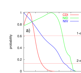
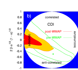
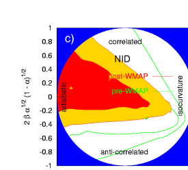
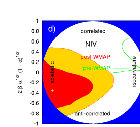
Figure 1: a) the likelihood function of the isocurvature fraction $\alpha$, for the three different types of uncorrelated isocurvature modes (i.e., with the prior $\beta=0$); b) the 1- and 2-$\sigma$ contours of $\alpha$ and the cross-correlated mode coefficient $2\beta\sqrt{\alpha(1-\alpha)}$, for the CDM isocurvature mode: the small (red) contours are based on all the data, with one flat prior $n_{\rm iso}>0.6$, while the large (green) ones show the situation before WMAP, with an additional prior $\omega_{B}<0.037$; c) same as b) for NID; d) same as b) for NIV.

The CMB temperature fluctuations on large scales, the Sachs-Wolfe contribution, can be written as

$${\Delta T\over T}={1\over 3}\Phi^{\rm ad}_{\rm rad}+2\Phi^{\rm iso}_{\rm rad}={1\over 5}{\cal R}_{\rm rad}-{2\over 5}{\cal S}_{\rm rad}\,,$$ (10)

in terms of the initial conditions during the radiation era, $\Phi^{\rm ad}_{\rm rad}=(3/5){\cal R}_{\rm rad}$ and $\Phi^{\rm iso}_{\rm rad}=-(1/5){\cal S}_{\rm rad}$. However, in order to evaluate the temperature and polarization anisotropies seen in the CMB today, one has to calculate the radiation transfer functions for adiabatic and isocurvature perturbations, $g_{l}^{\rm ad}(k),\ g_{l}^{\rm iso}(k)$ and $g_{l}^{\rm corr}(k)$. The angular power spectrum for each individual mode is therefore

$$C_{l}^{\rm ad}\! \equiv \!{1\over 25}\,\int{dk\over k}\,g_{l}^{\rm ad}(k)\,\left({k\over k_{0}}\right)^{n_{\rm ad}-1}\,,$$

$$C_{l}^{\rm iso}\! \equiv \!{4\over 25}\,\int{dk\over k}\,g_{l}^{\rm iso}(k)\,\left({k\over k_{0}}\right)^{n_{\rm iso}-1}\,,$$

$$C_{l}^{\rm corr}\! \equiv \!-{4\over 25}\,\int{dk\over k}\,g_{l}^{\rm corr}(k)\,\left({k\over k_{0}}\right)^{(n_{\rm ad}+n_{\rm iso})/2-1}\,,$$

and the total angular power spectrum is computed as $\!{}^{{\bf?}}$

$$C_{l}=C_{l}^{\rm ad}+B^{2}\,C_{l}^{\rm iso}+2B\,\cos\Delta\,C_{l}^{\rm corr}\,,$$ (11)

where $A\equiv 1$ has been marginalized over, and $B$ is now the entropy to curvature perturbation ratio during radiation era, $B\equiv{\cal S}_{\rm rad}/{\cal R}_{\rm rad}$. We will use here a slightly different notation, used before by other groups $\!{}^{{\bf?},{\bf?}}$, where $A^{2}\equiv(1-\alpha)$ and $B^{2}\equiv\alpha$,

$$C_{l}=(1-\alpha)\,C_{l}^{\rm ad}+\alpha\,C_{l}^{\rm iso}+2\beta\,\sqrt{\alpha(1-\alpha)}\,C_{l}^{\rm corr}\,.$$ (12)

Here the parameter $\alpha$ runs from purely adiabatic ($\alpha=0$) to purely isocurvature ($\alpha=1$), while $\beta$ defines the correlation coefficient, with $\beta=+1/-1$ corresponding to maximally correlated/anticorrelated modes. There is an obvious relation between both parametrizations:

$$\alpha=B^{2}/(1+B^{2})\,,\hskip 28.45274pt\beta=\cos\Delta\,.$$ (13)

This notation has the advantage that the full parameter space of $(\alpha,\ 2\beta\sqrt{\alpha(1-\alpha)})$ is contained within a circle of radius $1/2$. The North and South rims correspond to fully correlated ($\beta=+1$) and fully anticorrelated ($\beta=-1$) perturbations, with the equator corresponding to uncorrelated perturbations ($\beta=0$). The East and West correspond to purely isocurvature and purely adiabatic perturbations, respectively. Any other point within the circle is an arbitrary admixture of adiabatic and isocurvature modes.

In order to compute the theoretical prediction for the $C_{l}$ coefficients of the temperature and polarization power spectra, as well as the matter spectra $P(k)$, for all four different components, we have used a CMB code developed by one of us (A.R.) which coincides, within 1% errors, with the values provided by CMBFAST for AD and CDI modes, and also includes the neutrino isocurvature modes as well as the cross-correlated power spectra. Note that the code defines the tilt of each power spectrum with respect to a pivot scale $k_{0}$ corresponding the present value of the Hubble radius, while CMBFAST uses $k_{0}=0.05$ Mpc^-1. Thus, the comparison of our results with those of WMAP $\!{}^{{\bf?}}$ for the CDI mixed model is not straightforward.

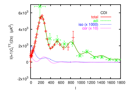
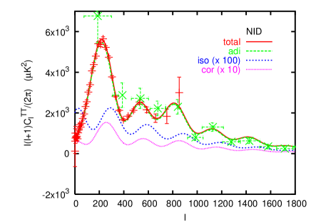
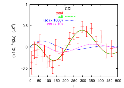
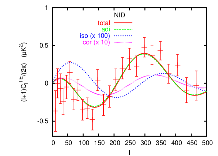
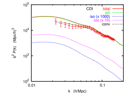
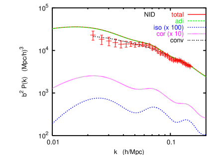
Figure 2: Some best fit models compared to data. The left plots correspond to correlated CDM isocurvature modes, the right plots to neutrino density isocurvature modes. The parameters of these models can be seen in Table 1. From top to bottom, we show the $C_{l}^{\rm TT}$, $C_{l}^{\rm TE}$ and $P(k)$ power spectra, as well as the contribution of each component: adiabatic (ad), isocurvature (iso), cross-correlated (corr). The last two components have been rescaled by a factor indicated in each figure. We also show the data points that we use throughout the analysis, from WMAP, ACBAR and 2dF. In the case of the matter power spectrum, we plot in addition the theoretical spectrum convolved with the experimental window function (conv), in order to allow for a visual comparison with the data (which is not possible directly with the unconvolved power spectrum, due to the shape of the window functions). Note that these two best-fit models are extremely close to the pure adiabatic one: the differences in the respective power spectra would be indistinguishable by eye.

Table 1: The best fit values of cosmological parameters for both adiabatic, mixed-isocurvature and correlated models, with their $\chi^{2}$ per degree of freedom.

model	$\omega_{\rm B}$	$\omega_{\rm cdm}$	$\Omega_{\Lambda}$	$n_{\rm ad}$	$n_{\rm iso}$	$\alpha$	$\beta$	$\chi^{2}/\nu$
AD	0.021	0.12	0.70	0.95	$-$	$-$	$-$	1478.8/1435
CDI	0.023	0.12	0.73	0.99	1.02	0.10	$-$	1478.3/1433
BI	0.023	0.12	0.73	0.99	1.02	0.72	$-$	1478.3/1433
NID	0.023	0.12	0.73	0.99	0.95	0.37	$-$	1478.2/1433
NIV	0.021	0.12	0.70	0.95	$-$	0.0	$-$	1478.8/1433
c-CDI	0.022	0.12	0.71	0.97	1.23	0.001	1.0	1478.0/1432
c-BI	0.022	0.12	0.71	0.97	1.23	0.03	1.0	1478.0/1432
c-NID	0.022	0.12	0.73	0.97	1.04	0.10	0.26	1477.7/1432
c-NIV	0.021	0.12	0.71	0.95	0.71	0.03	$-1.0$	1477.5/1432

Conclusions. Using the recent measurements of temperature and polarization anisotropies in the CMB by WMAP, as well as the matter power spectrum measured by 2dFGRS, one can obtain stringent bounds on the various possible isocurvature components in the primordial spectrum of density and velocity fluctuations. We have considered both correlated and uncorrelated adiabatic and isocurvature modes, and find no significant improvement in the likelihood of a cosmological model by the inclusion of an isocurvature component. For instance, a model allowed at the 2$\sigma$ level by the present observations (WMAP + ACBAR + 2dFGRS) with a correlated admixture of adiabatic and CDM isocurvature modes, with $\alpha=0.46$ and $\beta=-0.3$, and tilts $n_{\rm ad}=1.03$ and $n_{\rm iso}=0.79$, together with cosmological parameters $\Omega_{\Lambda}=0.744$, $\omega_{\rm cdm}=0.112$ and $\omega_{\rm B}=0.0246$, has a $\chi^{2}$ per d.o.f. of 1.0349, while the corresponding c-CDI best fit model (see Table. 1) has $\chi^{2}/\nu=1.0321$, and the pure adiabatic best fit model has $\chi^{2}/\nu=1.0305$. Therefore, we conclude that for the moment there is no significant improvement in the likelihood of a model by the inclusion of a small admixture of isocurvature perturbations. In other words, the basic paradigm of single field inflation passes for the moment all observational constraints with flying colors. It is expected $\!{}^{{\bf?}}$ that in the near future, with better data, we will be able to constrain further a possible isocurvature fraction, or perhaps even discover it.

References

References

- [1] A. D. Linde, Phys. Lett. B 158, 375 (1985); L. A. Kofman and A. D. Linde, Nucl. Phys. B 282, 555 (1987); S. Mollerach, Phys. Lett. B 242, 158 (1990); A. D. Linde and V. Mukhanov, Phys. Rev. D 56, 535 (1997); M. Kawasaki, N. Sugiyama and T. Yanagida, Phys. Rev. D 54, 2442 (1996); P. J. E. Peebles, Astrophys. J. 510, 523 (1999).
- [2] D. Polarski and A. A. Starobinsky, Phys. Rev. D 50, 6123 (1994); M. Sasaki and E. D. Stewart, Prog. Theor. Phys. 95, 71 (1996); M. Sasaki and T. Tanaka, Prog. Theor. Phys. 99, 763 (1998).
- [3] J. García-Bellido and D. Wands, Phys. Rev. D 53, 5437 (1996).
- [4] C. Gordon, D. Wands, B. A. Bassett and R. Maartens, Phys. Rev. D 63, 023506 (2001); N. Bartolo, S. Matarrese and A. Riotto, Phys. Rev. D 64, 123504 (2001).
- [5] D. Wands, N. Bartolo, S. Matarrese and A. Riotto, Phys. Rev. D 66, 043520 (2002).
- [6] F. Finelli and R. H. Brandenberger, Phys. Rev. D 62, 083502 (2000); F. Di Marco, F. Finelli and R. Brandenberger, Phys. Rev. D 67, 063512 (2003).
- [7] D. Langlois, Phys. Rev. D 59, 123512 (1999); D. Langlois and A. Riazuelo, Phys. Rev. D 62, 043504 (2000).
- [8] G. Efstathiou and J. R. Bond, Mon. Not. R. Astron. Soc. A 218, 103 (1986); 227, 33 (1987); P. J. E. Peebles, Nature 327, 210 (1987). H. Kodama and M. Sasaki, Int. J. Mod. Phys. A 1, 265 (1986); 2, 491 (1987); S. Mollerach, Phys. Rev. D 42, 313 (1990).
- [9] M. Bucher, K. Moodley and N. Turok, Phys. Rev. D 62, 083508 (2000); Phys. Rev. Lett. 87, 191301 (2001).
- [10] D. H. Lyth and D. Wands, Phys. Lett. B 524, 5 (2002); D. H. Lyth, C. Ungarelli and D. Wands, Phys. Rev. D 67, 023503 (2003).
- [11] P. Crotty, J. García-Bellido, J. Lesgourgues and A. Riazuelo, Phys. Rev. Lett. 91, 171301 (2003).
- [12] C. L. Bennett et al., Astrophys. J. Suppl. 148, 1 (2003); D. N. Spergel et al., Astrophys. J. Suppl. 148, 175 (2003); H. V. Peiris et al., Astrophys. J. Suppl. 148, 213 (2003).
- [13] C. l. Kuo et al., Astrophys. J. 600, 32 (2004);
- [14] J. H. Goldstein et al., Astrophys. J. 599, 773 (2003).
- [15] J. A. Peacock et al., Nature 410, 169 (2001); W. J. Percival et al., Mon. Not. R. Astron. Soc. A 327, 1297 (2001); 337, 1068 (2002).
- [16] R. Stompor, A. J. Banday and K. M. Gorski, Astrophys. J. 463, 8 (1996); P. J. E. Peebles, Astrophys. J. 510, 531 (1999); E. Pierpaoli, J. García-Bellido and S. Borgani, JHEP 9910, 015 (1999); M. Kawasaki and F. Takahashi, Phys. Lett. B 516, 388 (2001); K. Enqvist, H. Kurki-Suonio and J. Väliviita, Phys. Rev. D 62, 103003 (2000); 65, 043002 (2002).
- [17] R. Trotta, A. Riazuelo and R. Durrer, Phys. Rev. Lett. 87, 231301 (2001); Phys. Rev. D 67, 063520 (2003).
- [18] L. Amendola, C. Gordon, D. Wands and M. Sasaki, Phys. Rev. Lett. 88, 211302 (2002).
- [19] C. Gordon and A. Lewis, Phys. Rev. D 67, 123513 (2003); New Astron. Rev. 47, 793 (2003).
- [20] J. Valiviita and V. Muhonen, Phys. Rev. Lett. 91, 131302 (2003).
- [21] R. Trotta and R. Durrer, arXiv:astro-ph/0402032.