Search for Cosmic Strings in CMB Anisotropies

Abstract

We have searched the 1st-year WMAP W-Band CMB anisotropy map for evidence of cosmic strings. We have set a limit of $\delta=8\pi G\mu/c^{2}<8.2\times 10^{-6}$ at 95% CL for statistical search for a significant number of strings in the map. We also have set a limit using the uniform distribution of strings model in the WMAP data with $\delta=8\pi G\mu/c^{2}<7.34\times 10^{-5}$ at 95% CL. And the pattern search technique we developed here set a limit $\delta=8\pi G\mu/c^{2}<1.54\times 10^{-5}$ at 95% CL.

1 Introduction

Current theories of particle physics predict that topological defects would almost certainly be formed during the early evolution of the universe [1]. Just as liquids turn to solids when the temperature drops, so the interactions between elementary particles run through distinct phases as the typical energy of those particles decreases with the expansion of the universe. When conditions favor the appearance of a new phase, the new phase crops up in many places at the same time, and when separate regions of the new phase run into each other, topological defects are the result. The detection of defects in the modern universe would provide precious information on events in the earliest moments after the Big Bang. Their absence, on the other hand, would force a major revision of current physics theories. The least of which would be to have the phase transitions be second or higher order.

The potential role of cosmic topological defects in the evolution of our universe has interested the astrophysical community for many years. Combined theoretical and experimental work has led to the development of observational signatures in a variety of diverse data sets. These have, on one hand removed one major motivation of the primary role in structure formation and on the other raised new motivations. These have also narrowed the range of allowable topological defects so that most viable models are likely to produce some variety of cosmic strings.

CMB anisotropy power spectrum observations rule out topological defects as the primary source of structure in the universe [2,3]. Observations strongly favor adiabatic random fluctuations from something like inflation rather than the structure formation from topological defects (e.g. cosmic strings). These CMB results, while confirming inflation, do not rule out lower level contributions from topological defects. Interest in cosmic strings has, in fact, been renewed with recent theoretical work on hybrid inflation, D-Brane inflation and SUSY GUTS. The idea that inflationary cosmology might lead to cosmic string production is not new; however, it has received new impetus from the brane world scenario suggested by superstring theory. A seemingly unavoidable outcome of brane inflation is the production of a network of cosmic strings [4], whose effects on cosmological observables range from negligible to substantial, depend on the specific brane inflationary scenario [5]. A number of theory papers [12,13,14], anticipating that searches from cosmic strings will be negative and set significant limits, have begun developing modified theories so as not to produce them. At minimum these modified models must introduce a new field (also warping brane).

Since a moving string would produce a steplike discontinuity in the CMB, it will cause temperature distribution deviate from Gaussian. We may be able to detect non-Gaussian aspects of temperature distribution provided sufficient resolution. We search for strings in two ways: statistical and pattern-discovery methods. Statistical analysis determines how much the distribution of temperature fluctuation deviates from Gaussian distribution or what fraction of the fluctuations might be due to strings. In the second approach, we can search for cosmic strings directly from temperature map by their distinctive pattern of anisotropy. The latter approach is much easier and more straight forward when CMB signal is not contaminated seriously. These methods are distinctly different than a simple fitting to angular power spectrum [4].

2 Effect of Cosmic Strings on CMB

2.1 Signal from a moving Cosmic String

Consider a cosmic string with mass per unit length $\mu$, velocity $\vec{\beta}$ and direction $\hat{s}$ both of which are perpendicular to the line of sight and is backlighted by a uniform blackbody radiation background of temperature $T$. Due to its angular defect $\delta=8\pi G\mu/c^{2}$, there is a Doppler effect of one side of the string relative to the other which causes a temperature step across the string [8,9]

$$\frac{\delta T}{T}=8\pi G\mu\gamma\beta/c^{2}.$$ (1)

where $\gamma=1/\sqrt{1-\beta^{2}}$. This expression was generalized for arbitrary angles between the string direction $\hat{s}$, its velocity $\vec{\beta}$, and the line of sight $\hat{n}$ [6,7]

$$\frac{\delta T}{T}=8\pi G\mu\gamma\beta\hat{n}\cdot(\hat{\beta}\times\hat{s})/c^{2}.$$ (2)

2.1.1 Probability distributions for relevant parameters

Figure 1: Probability distributions for temperature steps in equation (2). The solid curve represents the probability with both string direction $\hat{s}$ and string velocity $\vec{\beta}$ having random directions while the flat dotted line assumes $\hat{\beta}\bot\hat{s}$ ($\sin\phi=1$) but the direction of $\hat{\beta}\times\hat{s}$ is random relative to the line of sight ($\cos\theta$ random).

$\delta T/T$ in equation (2) is determined by three factors $G\mu/c^{2}$, $\gamma\beta$ and $\hat{n}\cdot(\hat{\beta}\times\hat{s})$ which arise from different sources. $G\mu/c^{2}$ is related to symmetry breaking scale, we can assume $\gamma\beta\sim 1$ except near cusps where one can have $\gamma\gg 1$ and $\hat{n}\cdot(\hat{\beta}\times\hat{s})$ depends on the combination of relative angles among $\hat{\beta}$, $\hat{s}$ and $\hat{n}$. We can also assume that $\hat{\beta}\times\hat{s}$ is random in direction to the line of sight $\hat{n}$ in 3-D space. If we denote $\hat{\beta}\times\hat{s}$ as $\hat{u}\,\sin\phi$, then

$$\hat{n}\cdot(\hat{\beta}\times\hat{s})=\hat{n}\cdot\hat{u}\,\sin\phi=\cos\theta\,\sin\phi\;.$$ (3)

The infinitesimal probability that $\cos\theta$ has an arbitrary value is $2\pi\sin\theta d\theta/4\pi=\frac{1}{2}d\cos\theta$ and thus its probability distribution is uniform in $\cos\theta$. If the string velocity $\vec{\beta}$ and its direction $\hat{n}$ are uncorrelated, the probability distribution for $\sin\phi$ is $y$ is $y/\sqrt{1-y^{2}}$. Then, the probability distribution for $k\equiv\hat{n}\cdot(\hat{\beta}\times\hat{s})$ being an arbitrary value $-1<k<1$ becomes, substituting $\cos\theta=x$,

$$P(k) = \int^{1}_{-1}\frac{1}{2}dx\int^{1}_{0}\frac{y}{\sqrt{1-y^{2}}}\delta(k-x\,y)dy$$ (4)

$$= \frac{1}{2}\int^{1}_{|k|}\frac{k\,dx}{x\sqrt{x^{2}-k^{2}}}$$

$$= \frac{1}{2}\cos^{-1}|k|\,.$$

Often string velocity and direction will be perpendicular to each other so that $\sin\phi\simeq 1$ and in this case the probability reduces to $P(k)=\frac{1}{2}$. These probability distributions are plotted in Figure 1.

In a matter dominated universe the projected angular length of string in the redshift interval [$z_{1},~{}z_{2}$] scales as $\sqrt{z_{1}}-\sqrt{z_{2}}$ [10]. The standard cosmological model ($\Omega_{DE}\sim 0.7,\>\Omega_{m}\sim 0.3$) gives $z_{ls}\sim 1100$ [10]. The apparent angular size of the horizon at the CMB last scattering redshift $z_{ls}$ is

$$\theta_{H}=\frac{1}{\sqrt{z_{ls}}}radians=1.8^{\circ}\left(\frac{1000}{z_{ls}}\right)^{1/2}\sim 1.7^{\circ}.$$ (5)

The average distance between strings is roughly $d_{H}/3$. Thus the typical angular distance between the discontinuities on the sky to be of the order of $\theta_{H}$. The rough expected magnitude of the jumps in temperature are of order $\delta T/T\sim 13G\mu/c^{2}~{}{\rm to}~{}19G\mu/c^{2}$. With angular resolution of $2^{\prime}$ (2 arcmin) there could be sharp jumps up to about $\delta T/T\sim 40G\mu/c^{2}$. (i.e. peak range of temperature steps in a distribution of possible steps.) If the angular resolution is poorer, then the blurring effectively smooths the steps that the maximum range of steps are at a somewhat smaller level.

2.2 Statistical Fluctuations

Figure 2: Temperature Distribution of full sky from WMAP. Pixels with $|\Delta T|>1mK$ or $|$Galactic latitude$|<10^{\circ}$ are excluded because these signals are mainly due to the Galaxy or bright sources. The dashed curve is the best-fitted Gaussian with $\mu=23.6\mu K$ and $\sigma=201.25\mu K$. $\chi^{2}/DOF$ for the Gaussian fit is 4085.87/398 and the solid curve represents 2.6M-Gaussians fit with $\mu=23.6\mu K$, $\sigma_{0}=6682.22\mu K$ and $\sigma_{CMB}=80.25\mu K$. $\chi^{2}/DOF$ for 2.6M-Gaussians fit is 435.76/398.

The signal in a microwave sky map will be made of several components: noise from the instrument, foreground signals (expected to be small away from the galactic plane and with strong sources punched out), CMB fluctuations from adiabatic (or appropriate) fluctuations, and potential signals from the strings.The signal observed at any pixel is then

$$T_{pixel}=Noise_{pixel}+T_{foreground}+\delta T_{CMB}+\delta T_{string}.$$ (6)

Since the nature of signal is the superposition of random Gaussian signal (noise, $\delta T_{CMB}$) and non-Gaussian contribution ($\delta T_{string}$), there are two basic forms of distribution functions (foreground will be removed from the beginning).

Here and later on in this paper, we use two identical variables $T$ and $\Delta T$ confusingly, i.e, $T=\Delta T=T_{absolute}-T_{0}(2.73K)$.
(1)Gaussian signal
Major portion of CMB signal obeys Gaussian distribution,

$$f_{1}(T) = \frac{1}{\sigma\sqrt{2\pi}}e^{-\frac{1}{2}{\left(\frac{T-\mu}{\sigma}\right)}^{2}}$$ (7)

$$\sigma^{2} = \sigma^{2}_{0}/n_{i}+\sigma^{2}_{CMB}$$

where $\sigma_{0}$ and $\sigma_{CMB}$ are variances from noise and CMB fluctuations each, $n_{i}$ is the number of observations for $i_{\mathrm{th}}$ pixel. We make use of the information that the noise is Gaussian (actually Gaussian per observation and thus variance inversely proportional to the number of observations per pixel) and the intrinsic CMB fluctuations are gaussianly distributed.
(2)Non-Gaussian signal from strings
When a straight moving string is added to a region, we can expect a temperature distribution that is the sum of two Gaussians rather than single Gaussian because of the blue- and redshift by a transversely moving string. Then the probability distribution in equation (7) is modified to

$$f_{2}(T)=\frac{1}{\sigma\sqrt{2\pi}}\left[p\,e^{-\frac{1}{2}{\left(\frac{T-\mu-\delta T/2}{\sigma}\right)}^{2}}+q\,e^{-\frac{1}{2}{\left(\frac{T-\mu+\delta T/2}{\sigma}\right)}^{2}}\right]$$ (8)

where $p=N_{blue}/N_{total}$, the ratio blueshifted pixels to total pixels, $q=1-p$ and $\delta T/2$ is half of the effective height of step across the string as given in equation (2). If we denote $\nu$ and $\sigma_{obs}$ as mean and standard deviation calculated from observation, they are related to $\mu$ and $\sigma$ as follows

$$\nu = \mu+p\,\delta T/2+(1-p)(-\delta T/2)$$ (9)

$$= \mu+(2p-1)\delta T/2$$

$$\sigma_{obs}^{2} = <(T-\nu)^{2}>$$ (10)

$$= \int^{\infty}_{-\infty}(T-\nu)^{2}f_{2}(T)\,dT$$

$$= \sigma^{2}+4p(1-p)(\delta T/2)^{2}\;.$$

Here we used an approximation on the integration interval as $-1mK<T<1mK\longrightarrow-\infty<T<\infty$. It is a good approximation because, $\sigma\sim 200\mu K$ and thus $1mK\sim 5\sigma$, the variance integral in equation (10) over $[-5\sigma,5\sigma]$ covers 99.9985% of that over $[-\infty,\infty]$. This approximation is also implied in equation (19).

Signal	Limit $\sigma_{string}$	$\delta T/T$	Limit $G\mu/c^{2}$	GUT symmetry breaking
	$\mu$K	$\delta=8\pi G\mu\gamma\beta/c^{2}$	$\times 10^{6}$	scale $\eta_{SB}$ ($\times 10^{16}$GeV)
Total	201.25	7.37 $\times 10^{-5}$	2.93	2.05
Total - Noise 6.7mK/obs	80.26	2.94$\times 10^{-5}$	1.17	1.30
Total - Noise - Adiabatic CMB	22.49	0.82 $\times 10^{-5}$	0.33	0.69
Uniform Distribution of Strings	57.82	7.34$\times 10^{-5}$	2.92	2.05
Pattern Search	N/A	1.54$\times 10^{-5}$	0.61	0.94

Table 1: Variance Limits on Cosmic Strings. All the values presented are at 95% CL. The model ’Uniform Distribution of Strings’ on the fourth row is the distribution given in the equation (18). The GUT symmetry breaking scales, $\eta_{SB}$, in the last column are calculated using the relation $\eta_{SB}\sim m_{pl}\sqrt{G\mu/c^{2}}$ with $m_{pl}=1.2\times 10^{19}$GeV.

Temperature distribution of sky may be explained with appropriate combinations of $f_{1}(T)$ and $f_{2}(T)$. All the models introduced in the following sections are based on these two primary patterns of temperature distribution.

2.2.1 Variance: Quadratic Estimator Test for String Contribution

Assuming that the signals are all statistically independent, we can find the variance in the map

$$\sigma^{2}_{S}=\sigma^{2}_{noise}+\sigma^{2}_{foreground}+\sigma^{2}_{CMB}+\sigma^{2}_{string}$$ (11)

We remove the significant foreground contribution by dropping pixels with $|$Galactic latitude$|<10^{\circ}$ or $|\Delta T|>1mK$. The first condition is to exclude galactic area where non-CMB signal is dominant. We lose 217 more pixels by imposing the condition $|\Delta T|<1mK$, 4 pixels are less than $-1mK$ and 213 pixels are greater than $1mK$. Since Gaussian tail probability allows $\sim 1.7$ pixels in $|\Delta T|>1mK$ region and they mostly form clusters, we can drop those pixels as they are from unusual bright sources. We introduce a temperature distribution based on the Gaussianity of signal for each pixel in WMAP 1st-year data and calculate $\sigma_{CMB}$ which contains all the contributions except instrumental noise,

$$f_{2.6M}(T)\! = \!\frac{1}{N}\sum_{i}\frac{1}{\sigma_{i}\sqrt{2\pi}}e^{-\frac{1}{2}{\left(\frac{T-\mu}{\sigma_{i}}\right)}^{2}}$$

$$\sigma^{2}_{i}\! = \!\frac{\sigma_{0}^{2}}{n_{i}}+\sigma^{2}_{CMB}$$ (12)

where $N$ is the total number of pixels, 2,598,695, $i$ is pixel number with maximum resolution of WMAP 1st-year data, $\sigma_{0}^{2}$ is variance due to noise per measuremet and $n_{i}$ is effective number of measurements for $i_{th}$ pixel. The distribution $f_{2.6M}(T)$ in equation (2.2.1) has minimum $\chi^{2}$ for $\sigma_{CMB}=80.25^{+0.05}_{-1.65}\mu K$ and $\sigma_{0}=6682.22^{+21.78}_{-3.22}\mu K$ and thus $\sigma_{S}=200.68^{+0.57}_{-0.74}\mu K$ each with 95$\%$ CL. This observation in turn allows an upper limit of order $\sigma_{string}\stackrel{{\scriptstyle<}}{{\sim}}200\mu K$ and thus providing a limit of $8\pi G\mu/c^{2}\stackrel{{\scriptstyle<}}{{\sim}}200\mu K/2.73K=73.5\times 10^{-6}$.

We obtain a better upper limit, if we know the mean contribution of instrumental noise and other signals. According to the WMAP 1st-year data release, the sum over pixels of (number of measurements per pixel)^-1 for 2,598,695 pixels included here is 1968.96. Thus the effective variance due to noise is

$$\sigma^{2}_{noise}\! = \!(\sigma^{2}_{0}\sum_{i}\frac{1}{n_{i}})/N$$ (13)

$$= \!(6682.22^{+21.78}_{-3.22})^{2}\frac{1968.96}{2598695}$$

$$= \!(183.93^{+0.6}_{-0.08}\>\mu K)^{2},\;95\%\;{\mathrm{CL}}$$

where $n_{i}$ is the effective number of measurements for $i_{th}$ pixel.

Figure 3: Temperature distribution of full sky excluding the pixels with $|$Galactic latitude$|<10^{\circ}$ or $|\Delta T|>1mK$. Solid curve represents the best-fitted curve of uniformly distributed strings model and the dotted curve shows actual WMAP 1st-year data.

Under the assumption that the signals other than noise and from strings are negligible,

$$\sigma^{2}_{string}\leq\sigma^{2}_{S}-\sigma^{2}_{noise}=(80.25^{+0.05}_{-1.65}\>\mu K)^{2},\;95\%\;{\mathrm{CL}}.$$ (14)

And we are able, by taking the instrument noise into account, to set a lower upper limit.

Figure 4: $\chi^{2}$ distribution for the uniformly distributed strings model. $\chi^{2}_{min}=435.43$ with 398 degrees of freedom. Parameters span $0<\delta T<200.3\,\mu K$ and $192.1\,\mu K<\sigma<200.8\,\mu K$ at 95% CL. Here $\sigma^{2}$ represents the total variance except string contribution, $\sigma^{2}=\frac{\sigma^{2}_{0}}{N}\sum_{i}1/{n_{i}}+\sigma^{2}_{CMB}$. The outer contour is for 95% CL which is almost overlapped with the 68% CL contour in vertical direction.

Taking into account the CMB anisotropy spectrum is characteristic of anisotropies that arise from stochastic, Gaussianly-distributed, adiabatic primordial perturbations. We decompose the variance $\sigma^{2}_{CMB}$ computed in equation (14) into two contributions, one from adiabatic fluctuation and one from strings, $\sigma^{2}_{CMB}=\sigma^{2}_{adiabatic}+\sigma^{2}_{string}$. Since $\sigma^{2}_{CMB}=\sum_{l}(2l+1)C_{l}B_{l}^{2}/4\pi$ and string contribution in $C_{l}$ is $\sim 10\%$ [4] where $B_{l}$ is beam filter function, we estimate the upper limit of $\sigma^{2}_{string}\sim\sigma^{2}_{CMB}/10=(25.38^{+0.50}_{-1.04}\>\mu K)^{2}$, thus

$$0<\sigma_{string}<25.38^{+0.50}_{-1.04}\mu K,\;95\%\;{\mathrm{CL}}.$$ (15)

We can also calculate $\sigma_{adiabatic}^{2}$ directly from the relation between $\sigma_{CMB}^{2}$ and the power spectrum coefficients $C_{l}$. Using the $C_{l}$’s of best-fitted modeled cosmological parameters ($\Omega_{\Lambda}=0.73,\;\Omega_{b}=0.046,\;\Omega_{cdm}=0.224)$, $B_{l}$’s from WMAP 1st-year data and convolving with finite pixel size, we have

$$\sigma_{CMB}^{2}\!\! = \!\!\frac{1}{4\pi}\sum_{l}(2l+1)C_{l}B_{l}^{2}$$ (16)

$$= \!\!(79.085\pm 0.376\mu K)^{2},\;95\%\;{\mathrm{CL}}.$$

for beam and finite pixel size. Assuming that $\sigma_{CMB}^{2}$ in equation (16) is solely from adiabatic fluctuation, we have even lower upper limit on $\sigma_{string}$,

$$\sigma_{string}^{2} \!\leq\>\sigma^{2}_{S}-\sigma^{2}_{noise}-\sigma^{2}_{adiabatic}$$ (17)

$$= \!\!\!\!\!(201.25\mu K)^{2}-(183.85\mu K)^{2}-(78.709\mu K)^{2}$$

$$= \!\!\!\!\!(22.49\mu K)^{2},\;95\%\;{\mathrm{CL}}.$$

Both of these last two are model dependant as one could refit all cosmological parameters to include a small addition of string. Presumably that is what was done in [4].

2.2.2 Statistical Test for Temperature Step Expected from Random Strings

Figure 5: Generating the vector field $\vec{L}$. Pixels left demoted to middle pixels, middle $\rightarrow$ right: defining gradient of temperature $\nabla T$ and $\vec{L}$ which lies along temperature step.

For the anticipated distribution of strings, one would expect a random distribution of temperature steps which has roughly equal probability between the plus and minus the maximum temperature step amplitude. We also fitted to a distribution that was a Gaussian for the other signals convolved with a uniform distribution of temperature steps. Let ${\delta T_{0}}=8\pi G\mu\gamma\beta/c^{2}T_{0}$ be the characteristic value for a string, then the actual effect of temperature step left on the measured CMB is $k{\delta T_{0}}/2$ where $-1<k=\cos\theta\,\sin\phi<1$ from the equation (4) and $T_{0}=2.73K$. Assuming $\sin\phi\sim 1$ $i.e$ direction of a string and its velocity are most likely perpendicular, we have $P(k)\sim\frac{1}{2}$. Then, we obtain the distribution function of temperature

$$f_{T}(T)=\frac{1}{N}\sum_{i}\int^{1}_{-1}f_{2}^{(i)}(T,k{\delta T_{0}}/{2},\sigma)dk$$ (18)

where $f_{2}^{(i)}(T,k{\delta T_{0}}/{2},\sigma)$ is the two-Gaussians form with $p=0.5$ and $\delta T=k{\delta T_{0}}$ of $i$-th Gaussian in equation (2.2.1). Then, the apparent variance $\sigma_{uniform}^{2}$ for this distribution becomes, in terms of $\sigma$ and ${\delta T_{0}}$,

$$\sigma_{uniform}^{2}\!\! = \!\!<(T-\mu)^{2}>$$ (19)

$$= \!\!\int^{\infty}_{-\infty}(T-\mu)^{2}f_{T}(T)dT$$

$$= \!\!\frac{\sigma^{2}_{0}}{N}\sum_{i}\frac{1}{n_{i}}+\sigma^{2}_{CMB}+\frac{\delta T_{0}^{2}}{12}$$

where the first 2 terms are directly from the equation (2.2.1) and the last term is the contribution















from strings. From the $\chi^{2}$ distribution in Figure 4, we have $192.1\,\mu K<\sigma<200.8\,\mu K$ and $0<\delta T_{0}<200.3\,\mu K$ at $95\%$ CL. Thus, temperature variation by a moving string can be limited to, in terms of deficit angle,

$$0<\frac{\delta T_{0}}{T_{0}}=\frac{8\pi G\mu}{c^{2}}<7.34\times 10^{-5}\;,\;95\%{\mathrm{CL}}.$$ (20)

2.3 Search for Temperature Steps

One can directly search for temperature steps from the CMB sky map by their topological configuration or pattern. We define an algorithm to search for CMB temperature steps produced by cosmic strings in a background of CMB adiabatic fluctuations and (at present even more dominant) receiver noise. (For the WMAP 1st-year data release the signal-to-noise ratio for an average W-band pixel is about 0.5.) As a smoothing process, we demote $2^{2n}$ pixels of maximum resolution to one pixel with representative temperature value (average) assigned. This demoted pixel can be obtained by repeating demotion process shown in Figure 5 until we reach desired value of signal/noise. Since $\sigma_{S}\sim 201\mu K$ and $\sigma_{noise}\sim 184\mu K$ for the WMAP 1st-year data, it is reasonable to take 16 pixels demotion or more because we have $\sigma_{S}^{\left(16\right)}\sim 104\mu K$ and $\sigma_{noise}^{\left(16\right)}=\sigma_{noise}/\sqrt{16}\sim 46\mu K$, thus the contribution from noise becomes subdominant. Then a vector can be derived out of 4 neighboring demoted pixels. $\nabla T$ is defined as

$$(\nabla T)_{x} = \frac{1}{2}\left(T_{2}+T_{4}-T_{1}-T_{3}\right)$$ (21)

$$(\nabla T)_{y} = \frac{1}{2}\left(T_{3}+T_{4}-T_{1}-T_{2}\right)\;.$$ (22)

Figure 6: $\vec{L}$ field for the full sky with 64-pixel demotion. The center of the map is ($\theta=0^{\circ}$, $\phi=0^{\circ}$) in Galactic coordinates. Each arrow represents local temperature step and the temperature steps greater than $100\mu K$ are set to $100\mu K$. The pattern along the equator is due to the Galaxy.

We build up a vector field for the full sky which contains $12\times 2^{16-2n}$ $\nabla T$’s where $2^{2n}$ is the demotion factor. For each $\nabla T$, the perpendicular direction to $\nabla T$ represents the direction of step discontinuity. So if there is a consistent elongated line of discontinuity, we may interpret it as the signal due to moving string. After covering full sky with $\nabla T$-field, we rotate the vector field $-\pi/2$ to define $\vec{L}$-field so that each arrow lies along the local isothermal line with lefthand side of arrow being higher temperature. Figure 6 shows the $\vec{L}$-field map for the entire sky. The length of each arrow represents the magnitude of temperature gradient on that point and any temperature step greater than $100\mu K$ is set to $100\mu K$ to make steps visible which are less than $100\mu K$. It shows a long coherent structure along the galactic plane, this is because there is a steep temperature rise approaching the galactic plane.

2.4 Evaluating String Pattern

We define the connectedness of two neighboring temperature steps with two smoothness conditions for the heights of steps and the curve that links neighboring $\vec{L}$’s.
(1) Component Definition of Connectedness
We assume that the temperature distribution of WMAP 1st-year data is approximately Gaussian (Figure 2), $f_{T}(T)=(\sigma_{S}\sqrt{2\pi})^{-1}e^{\frac{1}{2}(\frac{T-\mu}{\sigma_{S}})^{2}}$ with $\mu\simeq 25\mu K$ and $\sigma_{S}\simeq 200\mu K$. Starting with this temperature distribution $f_{T}(T)$, after taking $n$-pixel demotion, we can derive the distributions of $L_{x}$ and $L_{y}$,

$$f_{comp}(L_{x})=\frac{1}{\sigma_{n}\sqrt{2\pi}}e^{-\frac{L^{2}_{x}}{2\sigma^{2}_{n}}}$$ (23)

where $\sigma^{2}_{n}$ is the variance for temperature distribution for $n$-pixel demoted pixels for example, $\sigma_{16}\simeq 104\mu K$. $L_{y}$ also has almost same distribution as equation (23), so we use equation (23) for both $L_{x}$ and $L_{y}$. This gives the probability distribution function for change of $x$-component, $\Delta_{x}\equiv L_{x}^{i}-L_{x}^{i+1}$,

$$f_{\Delta_{x}}(\Delta_{x})=\frac{1}{2\sigma_{n}\sqrt{\pi}}e^{-\frac{\Delta^{2}_{x}}{4\sigma^{2}_{n}}}.$$ (24)

and the same function for $y$-component. Since a pattern formed by moving string should have relatively constant height of step along the curve of pattern, we can impose a condition for connectedness as

$$|\Delta_{x}|<\Delta L_{c},\>\>|\Delta_{y}|<\Delta L_{c}$$ (25)

then, the probability that two adjacent vectors $\vec{L}_{i}$ and $\vec{L}_{i+1}$ meet these conditions is given by

$$P_{i,i+1} = \left[\int^{\Delta L_{c}}_{-\Delta L_{c}}f_{\Delta_{x}}(\Delta_{x})d\Delta_{x}\right]^{2}$$ (26)

$$= \left[erf(\frac{\Delta L_{c}}{2\sigma_{n}})\right]^{2}$$

where $\Delta L_{c}$ is the maximum value allowed for $\Delta_{x}$ and $\Delta_{y}$.

We set another condition for connectedness

$$\theta_{i,i+1}\equiv\cos^{-1}(\hat{D}_{i}\cdot\hat{D}_{i+1})<\theta_{c}$$ (27)

for a sequence to avoid too sharp turns (Figure 7) where $\theta_{c}$ is the maximum angle allowed for $\theta_{i,i+1}$ to claim $\vec{L}_{i}$ and $\vec{L}_{i+1}$ are connected. Figure 8 and 9 show examples of patterns which comply the definition described in equations (25) and (27) found in the WMAP 1st-year data. Here, we set $\Delta L_{c}=\sigma_{16}=104\mu K$ and $\theta_{c}=\pi/6$.

Figure 7: Relative angles defined for connectedness. $\hat{D}_{i}$ is a unit vector along the line that connects $\vec{L}_{i-1}$ and $\vec{L}_{i}$. $\theta_{i,i+1}$ is defined by the angle between $\hat{D}_{i}$ and $\hat{D}_{i+1}$, $\theta_{i,i+1}\equiv\cos^{-1}(\hat{D}_{i}\cdot\hat{D}_{i+1})$

.

Figure 8: A long temperature discontinuity pattern found at $(l=45^{\circ}$, $b=43^{\circ})$ in Galactic coordinates. The vector field is derived from 16-pixel demoted temperature sky map. This sequence has its maximum likelihood defined in the equation (28) at $\delta T=12\mu K$.

Figure 9: A short pattern with 16-pixel demotion from WMAP 1st-year data located at $l=127^{\circ}$, $b=20^{\circ}$ in Galactic coordinates. $\delta T_{opt}$ for this pattern is $0\mu K$, i.e, no preferred bias is found which is against its apparent feature. This is because the temperature step vectors on the left-half of the curve have wrong direction relative to expected string velocity at this part while those on the right-half are aligned correctly and these two opposite contributions cancel out the bias.

(2) Likelihood of sequence
Given that a sequence of temperature steps defined in the previous paragraph, we can estimate its likelihood for a signal due to a moving string. If a long temperature step is formed solely by a moving string, the $\vec{L}$’s assigned on the curve should be tangent to the curve. After allowing contamination by noise, adiabatic fluctuation or by other possible sources, each $\vec{L}$ on the curve will be off from local tangent. But if the contamination is not overwhelming, there should be still a bias seeded by string. We define the bias of a sequence with $N$-connected arrows quantitatively in terms of relative likelihood function as follows

$${\cal{L}}^{\left(N\right)}_{bias}(\delta T) = \prod^{N}_{i=1}e^{-\left(\vec{L_{i}}-\phi_{i}\vec{\delta T_{i}}\right)^{2}/2\sigma^{2}_{n}}$$ (28)

$$\phi_{i} = \left\{\begin{array}[]{r@{\quad:\quad}l}+1&{\mathrm{right\!-\!handed\>curve}}\\ 0&{\mathrm{straight\>line}}\\ -1&{\mathrm{left\!-\!handed\>curve}}\end{array}\right.$$ (32)

where $\vec{\delta T_{i}}$ is a tangent vector at $i_{th}$ grid point on the curve at which $\vec{L}_{i}$ is located and $|\vec{\delta T_{i}}|=\delta T$. $\phi_{i}$ is a phase factor defined at $i_{\mathrm{th}}$ grid point on the curve to give correct direction of string velocity on the curve. If the sequence turns right(left) locally at $i_{\mathrm{th}}$ grid, then $\phi_{i}=+1(-1)$ and it is zero when the sequence is straight at that point. On both the head and tail of a sequence, the phase factors are set to zero. This is an approximate prescription to describe realistic model of string motion. When $\vec{L_{i}}$’s are perfectly coincident with $\vec{\delta T_{i}}$, then ${\cal{L}}^{\left(N\right)}_{bias}(\delta T)$ become 1 and if $\vec{L_{i}}$’s are off by either direction or magnitude or both from $\vec{\delta T_{i}}$’s, then ${\cal{L}}^{\left(N\right)}_{bias}(\delta T)$ decays exponentially. So, if there is nonzero $\delta T$ that gives maximum ${\cal{L}}^{\left(N\right)}_{bias}(\delta T)$, then it is relatively more likely that there is a constant temperature step with height $\delta T$ imbedded in the sequence. Figure 10 shows the comparison of results between actual data (WMAP 1st-year data) and a simulated white noise. We can estimate from the curve the height of temperature discontinuity in equation (1),

$$\delta T\lesssim 42\mu K,\>\>95\%{\mathrm{CL}}$$ (33)

which is equivalent to symmetry breaking scale $\eta_{SB}\sim 0.94\times 10^{16}$GeV.

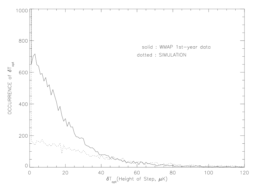
Figure 10: Distribution of $\delta T_{opt}$ at which likelihood function defined in equation (28) becomes maximum for a sequence. Each data set takes 16-pixel demotion. We included sequences which contain five or more arrows connected. There are many more sequences in the actual data than in the simulation which has identical size, mean and variance but white noise.

3 Conclusion

We have investigated WMAP 1st-year data to search directly or set limit on cosmic strings. For statistics of full sky map, we set the limit of contribution to variance by the strings as $0<\sigma_{string}<22.5\mu K$ which gives upper limit on deficit angle $0<\delta=8\pi G\mu/c^{2}<0.82\times 10^{-5}$. And we set up a model with a random distribution of strings with random orientation with which the relation between $\sigma_{string}$ and height of temperature step $8\pi G\mu\gamma\beta/c^{2}$ can be found. A limit on deficit angle is obtained from the model of uniform distribution of strings, $0<\delta=8\pi G\mu/c^{2}<7.34\times 10^{-5}$. This corresponds to symmetry breaking energy scale $\eta_{SB}\sim m_{pl}\sqrt{\frac{G\mu}{c^{2}}}\sim 2\times 10^{16}$GeV.

We developed a pattern search algorithm that can visualize the landscape of CMB temperature variation of the sky. There were some fairly long temperature rows but we didn’t find any compelling pattern of cosmic strings predicted by theory. Instead, by considering the distribution of heights of temperature discontinuities, we roughly estimated $0<\delta=8\pi G\mu/c^{2}<1.54\times 10^{-5}$ or equivalently $\eta_{SB}\sim 0.94\times 10^{16}$GeV.

The precision of data is yet to be refined and we expect WMAP 2nd-year data will provide much better chance to pin down the effects of topological defects on cosmic microwave background radiation and at that point refined analysis will be appropriate.

4 Acknowledgements

This work was supported by the U.S Department of Energy under Contract No. DE-AC03-76SF00098 at LBNL Physics Division and Physics Department at University of California, Berkeley. Some of the results in this paper have been derived using the HEALPix (Górski, Hivon, and Wandelt 1999). We would like to thank E. Canudas, K. Howley, J. Lamoreaux, T. Watari and L. Zuniga for discussion and comments.

References

• Jeannerot (2003) [1] R. Jeannerot, J. Rocher, M. Sakellariadou, astro-ph/0308134 (2003)
• (2) [2] H.V. Peiris, et al., astro-ph/0302225 (2003)
• (3) [3] L. Pogosian, S.-H. Henry Tye, I. Wasserman, M. Wyman, astro-ph/0304188 (2003)
• (4) [4] S. Sarangi and S-H.H. Tye, Phys. Lett. B536 (2002) 185, hep-th/0204074
• (5) [5] N. Jones, H. Stoica and S.-H.H. Type hep-th/0303269
• (6) [6] Vachaspati, T. 1986 ’Gravitational effects of cosmic strings’ Nucl. Phys. B277, 593.
• (7) [7] Vilenkin, A 1986 ”Looking for Cosmic Strings’, Nature 322, 613.
• (8) [8] Kaiser, N. & Stebbins, A. 1984 ’Microwave anisotropy due to cosmic strings’, Nature 310, 391.
• (9) [9] Gott, J.R. “Gravitational Lensing Effects of Vacuum String: Exact Results’ Ap. J. 288, 422.
• (10) [10] S. Bonometto, V. Gorini, U. Moschella Modern Cosmology IOP(2002)
• (11) [11] J. Lamoureaux, L.Zuniga, K. Howley, G. F. Smoot, “A New Technique for the Detection of Cosmic Strings in the GOODS Data”, in preparation (2004).
• (12) [12] J. Urrestilla, A. Ach\a’ucarro, A. C Davis, hep-th/0402032
• (13) [13] Taizan Watari, T. Yanagida, hep-ph/0402125
• (14) [14] Keshav Dasgupta, Jonathan P. Hsu, Renata Kallosh, Andrei Linde, Marco Zagermann, hep-th/0405247