The masses of the cataclysmic variables AC Cancri and V363 Aurigae
)
Abstract
We present time–resolved spectroscopy and photometry of the double–lined eclipsing cataclysmic variables AC Cnc and V363 Aur (= Lanning 10). There is evidence of irradiation on the inner hemisphere of the secondary star in both systems, which we correct for using a model that reproduces the observations remarkably well. We find the radial velocity of the secondary star in AC Cnc to be = 176 3 km s-1 and its rotational velocity to be = 135 3 km s-1. From these parameters we obtain masses of = 0.76 0.03 for the white dwarf primary and = 0.77 0.05 for the K2 1V secondary star, giving a mass ratio of = 1.02 0.04. We measure the radial and rotational velocites of the G7 2V secondary star in V363 Aur to be = 168 5 km s-1 and = 143 5 km s-1 respectively. The component masses of V363 Aur are = 0.90 0.06 and = 1.06 0.11 , giving a mass ratio of = 1.17 0.07. The mass ratios for AC Cnc and V363 Aur fall within the theoretical limits for dynamically and thermally stable mass transfer. Both systems are similar to the SW Sex stars, exhibiting single–peaked emission lines with transient absorption features, high–velocity S–wave components and phase–offsets in their radial velocity curves. The Balmer lines in V363 Aur show a rapid increase in flux around phase 0 followed by a rapid decrease, which we attribute to the eclipse of an optically thick region at the centre of the disc. This model could also account for the behaviour of other SW Sex stars where the Balmer lines show only a shallow eclipse compared to the continuum.
keywords:
accretion, accretion discs – binaries: eclipsing – binaries: spectroscopic – stars: individual: AC Cnc – stars: individual: V363 Aur – novae, cataclysmic variables.1 Introduction
Cataclysmic variables (CVs) are close binary stars consisting of a red dwarf secondary transferring material onto a white dwarf primary via an accretion disc or magnetic accretion stream. AC Cnc and V363 Aur are both examples of nova–likes (NLs), defined as CVs which have never been observed to undergo nova or dwarf–nova type outbursts. See ? for a comprehensive review of CVs.
A knowledge of the masses of the component stars in CVs is fundamental to our understanding of the origin, evolution and behaviour of these systems. Population synthesis models and the disrupted magnetic braking model of CV evolution can be observationally tested only if the number of reliably known CV masses increases. One of the most reliable ways to measure the masses of CVs is to use the radial velocity and the rotational broadening of the secondary star in eclipsing systems; the radial velocity of the disc emission lines may not represent the white dwarf’s orbital motion. At present, reliable masses are known for only 20 CVs, partly due to the difficulties in measurement (see ? for a review).
AC Cnc was classified as an eclipsing variable star by ? with an orbital period of 7.2 hours. ? suggested that AC Cnc is a NL based on colours, and the CV nature of AC Cnc was confirmed spectroscopically by ? through broad H and He emission lines and the later study of ?. ? discovered secondary star features in the spectra leading to the first mass determination by ?, who found = 0.82 0.13 and = 1.02 0.14 from the radial velocities of the primary and secondary components.
V363 Aur (= Lanning 10) was discovered by ? as a UV–bright source and later found to be a CV through broad Balmer and HeII emission by ?, and its typical CV energy distribution (?). ? obtained the first spectroscopic and photometric data, finding that V363 Aur is an eclipsing system with a period of 7.7 hours. ? calculated the component masses of V363 Aur to be = 0.86 0.08 and = 0.77 0.04 from the radial velocities of the HeII 4686Å emission line and the –band absorption.
The existing component masses of AC Cnc and V363 Aur use emission line radial velocity curves that exhibit phase shifts, suggesting that they could be unreliable. In addition to this, the mass ratio of AC Cnc found by ? of = 1.24 0.08 is the highest known of any CV and is very close to the upper limit of mass transfer stability computed by the models of ?. In this study, we present photometry and spectroscopy of AC Cnc and V363 Aur to calculate new masses using the secondary star properties alone.
2 Observations and Reduction
On the nights of 2001 January 9–14 we obtained blue and red spectra of AC Cnc and V363 Aur with the 2.5-m Isaac Newton Telescope (INT) + IDS spectrometer on La Palma. The blue setup comprised of the 235-mm camera with the R1200B grating and the EEV10 CCD chip, which gave a wavelength coverage of approximately 4490–5580Å at 0.95-Å (57 km s-1) resolution. In the red we used the 500-mm camera with the R1200Y grating and the TEK5 CCD chip resulting in a wavelength range of 6320–6720Å at a resolution of 0.8-Å (36 km s-1). Simultaneous photometry in the Johnson–Cousins and bands was recorded with the 1-m Jacobus Kapteyn Telescope (JKT) using the SITe2 CCD chip. Full phase coverage was achieved for both objects – a full journal of observations is given in Table 1, including the exposure times used.
We also collected 19 spectral type templates ranging from G5V–M2V, telluric stars to remove atmospheric features and flux standards on both the INT and JKT. Seeing varied between 1.0 and 1.5 arcsec over the observing run and conditions were photometric on all nights except for January 10 when some patchy cloud was present.
The spectra and images were reduced using standard procedures (e.g. ?; ?). Comparison arc spectra were taken every 40–50 min to calibrate instrumental flexure. The arcs were fitted with a sixth–order polynomial in blue and a fourth–order polynomial in red with rms scatters of better than 0.01Å. The photometry data were corrected for the effects of atmospheric extinction by subtracting the magnitude of a nearby comparison star (AC Cnc–9 and V363 Aur–3; ?) and using values obtained by the CAMC telescope (?). The absolute photometry is accurate to approximately 0.5 mJy; the relative photometry 0.03 mag. Slit losses were then corrected for by dividing each AC Cnc and V363 Aur spectrum by the ratio of the flux in the spectrum (summed over the whole spectral range) to the corresponding photometric flux.
| UT Date | Object | INT | No. of | Exposure | JKT | No. of | Exposure | UT | UT | Epoch | Epoch | ||||
|---|---|---|---|---|---|---|---|---|---|---|---|---|---|---|---|
| setup | spectra | time (s) | filter | images | time (s) | start | end | start | end | ||||||
| 2001 Jan 09 | V363 Aur | Red | 61 | 300 | 323 | 30 | 22: | 35 | 03: | 55 | 22915. | 74 | 22916. | 43 | |
| 2001 Jan 10 | V363 Aur | Blue | 39 | 400 | 272 | 30 | 20: | 07 | 04: | 36 | 22918. | 53 | 22919. | 63 | |
| 2001 Jan 11 | V363 Aur | Blue | 70 | 400 | 474 | 30 | 19: | 33 | 04: | 06 | 22921. | 57 | 22922. | 67 | |
| 2001 Jan 12 | V363 Aur | Red | 64 | 300 | 348 | 30 | 22: | 32 | 04: | 11 | 22925. | 97 | 22926. | 79 | |
| 2001 Jan 12 | AC Cnc | Red | 33 | 300 | 179 | 30 | 04: | 26 | 07: | 21 | –6. | 14 | –5. | 74 | |
| 2001 Jan 13 | AC Cnc | Red | 96 | 300 | 530 | 30 | 22: | 39 | 07: | 04 | –3. | 31 | –2. | 45 | |
| 2001 Jan 14 | AC Cnc | Blue | 90 | 300 | 521 | 30 | 22: | 27 | 06: | 33 | –0. | 32 | 0. | 80 | |
3 Results
3.1 Ephemeris
We derived new ephemerides for AC Cnc and V363 Aur, which are used to phase all data presented in this paper. The times of mid–eclipse were determined by fitting a parabola to the eclipse minima in the JKT data.
In the case of AC Cnc, a least–squares fit to the 29 eclipse timings listed in Table 2 (a) yields the ephemeris:
| (1) |
A least–squares fit to the 17 eclipse timings of V363 Aur listed in Table 2 (b) gives the ephemeris:
| (2) |
We see no evidence for any systematic variation in the O–C values shown in Table 2 in either AC Cnc or V363 Aur.
| (a) AC Cnc | |||||
| Cycle | HJD | O–C | Reference | ||
| (E) | at mid–eclipse | (secs) | |||
| (2,400,000+) | |||||
| –59456 | 34059. | 348 | –37. | 03 | KS80 |
| –50866 | 36640. | 446 | –336. | 27 | KS80 |
| –50813 | 36656. | 367 | –708. | 29 | KS80 |
| –47342 | 37699. | 327 | –474. | 74 | KS80 |
| –33860 | 41750. | 380 | 886. | 55 | KS80 |
| –31241 | 42537. | 320 | –20. | 02 | KS80 |
| –30136 | 42869. | 344 | –331. | 40 | KS80 |
| –29177 | 43157. | 504 | –149. | 38 | KS80 |
| –29074 | 43188. | 450 | –424. | 07 | KS80 |
| –29061 | 43192. | 362 | 76. | 43 | KS80 |
| –29038 | 43199. | 275 | 250. | 81 | KS80 |
| –28848 | 43256. | 368 | 447. | 87 | KS80 |
| –28785 | 43275. | 293 | 8. | 90 | KS80 |
| –28165 | 43461. | 579 | –857. | 79 | KS80 |
| –26867 | 43851. | 619 | 891. | 34 | KS80 |
| –26598 | 43932. | 439 | 162. | 19 | KS80 |
| –26588 | 43935. | 443 | 95. | 25 | KS80 |
| –26578 | 43938. | 448 | 114. | 72 | KS80 |
| –26525 | 43954. | 376 | 347. | 49 | KS80 |
| –23098 | 44984. | 1119 | 313. | 96 | YOK83 |
| –23094 | 44985. | 3141 | 339. | 02 | YOK83 |
| –23088 | 44987. | 1165 | 298. | 86 | YOK83 |
| –21522 | 45457. | 6637 | 254. | 17 | SKH84 |
| –19342 | 46112. | 7032 | 134. | 62 | Z87 |
| –19335 | 46114. | 8053 | 27. | 29 | Z87 |
| –19312 | 46121. | 7177 | 149. | 82 | Z87 |
| –6 | 51922. | 7339 | –8. | 03 | This Paper |
| –3 | 51923. | 6350 | –36. | 75 | This Paper |
| 0 | 51924. | 5367 | –13. | 63 | This Paper |
| (b) V363 Aur | |||||
| 0 | 44557. | 9495 | –168. | 03 | HLG82 |
| 3 | 44558. | 9128 | –204. | 81 | HLG82 |
| 6 | 44559. | 8772 | –146. | 54 | HLG82 |
| 105 | 44591. | 6813 | –46. | 80 | HLG82 |
| 106 | 44592. | 0023 | –67. | 70 | HLG82 |
| 4694 | 46065. | 8614 | 51. | 42 | SHK86 |
| 4700 | 46067. | 7877 | –48. | 05 | SHK86 |
| 4703 | 46068. | 7544 | 208. | 94 | SHK86 |
| 4706 | 46069. | 7182 | 215. | 37 | SHK86 |
| 9365 | 47566. | 3817 | 8. | 49 | RvPT92 |
| 9368 | 47567. | 3466 | 109. | 96 | RvPT92 |
| 10057 | 47788. | 6818 | 70. | 93 | RvPT92 |
| 10060 | 47789. | 6457 | 85. | 99 | RvPT92 |
| 10082 | 47796. | 7142 | 187. | 84 | RvPT92 |
| 10088 | 47798. | 6401 | 53. | 81 | RvPT92 |
| 22916 | 51919. | 5301 | –12. | 64 | This Paper |
| 22922 | 51921. | 4577 | 0. | 21 | This Paper |
3.2 Average Spectrum
The average spectra of AC Cnc and V363 Aur are shown in Fig. 1, and in Table 3 we list fluxes, equivalent widths (EW) and velocity widths of the most prominent lines measured from the average spectra.
Both systems show broad, symmetric, single–peaked Balmer emission lines instead of the double–peaked profiles one would expect from a high inclination accretion disc, much like other nova–like systems (e.g. ?). The HeI lines, however, are broad and double–peaked in nature. The line strength of HeII 4686Å is much stronger in V363 Aur than AC Cnc and even more dominant than H emission. Another high excitation feature, the CIII/NIII 4640–4650Å blend, is only present in V363 Aur and is very broad. The emission lines are characteristic of the SW Sex stars (e.g. ?), but unlike others in this sub–class, these systems show clear secondary star features (no doubt due to their longer periods and hence earlier type secondaries). Both AC Cnc and V363 Aur show the absorption features of the neutral metals CaI, FeI and MgI, even in the average spectrum shown in Fig. 1, which has not been corrected for orbital motion. The secondary star features appear to be stronger relative to the continuum in AC Cnc than in V363 Aur. The weak feature at 6614Å in the V363 Aur red spectrum is an interstellar absorption line.


|
| (a) AC Cnc | ||||||||
| Line | Flux | EW | FWHM | FWZI | ||||
| 10-14 | (Å) | (km s-1) | (km s-1) | |||||
| (ergs cm-2 s-1) | ||||||||
| H | 7.57 | 0.01 | 16.55 | 0.03 | 1100 | 100 | 2900 | 500 |
| H | 4.63 | 0.01 | 8.57 | 0.03 | 1250 | 100 | 2800 | 300 |
| HeI6678Å | 0.94 | 0.01 | 2.17 | 0.02 | 1100 | 100 | 1900 | 500 |
| HeII4686Å | 1.36 | 0.01 | 2.32 | 0.02 | 1600 | 100 | 2300 | 300 |
| (b) V363 Aur | ||||||||
| H | 8.07 | 0.02 | 11.82 | 0.02 | 1150 | 100 | 3100 | 500 |
| H | 3.60 | 0.02 | 4.88 | 0.02 | 1250 | 100 | 2900 | 300 |
| HeI6678Å | 0.86 | 0.01 | 1.31 | 0.02 | 1100 | 100 | 2300 | 500 |
| HeII4686Å | 4.84 | 0.02 | 6.19 | 0.03 | 1150 | 100 | 3400 | 500 |
| CIII/NIII4640–4650Å | 2.05 | 0.03 | 2.58 | 0.03 | 1950 | 100 | 4900 | 500 |
| HeII + CIII/NIII | 7.35 | 0.02 | 9.37 | 0.03 | ||||
3.3 Light Curves
The top panels of Fig. 2(a) and 2(b) show the and –band JKT light curves. The remaining panels show emission–line light curves, which were produced by subtracting a polynomial fit to the continuum and summing the residual flux. All light curves are plotted as a function of phase following our new ephemerides.
The and –band JKT light curves of AC Cnc show deep, symmetrical primary eclipses with out-of-eclipse magnitudes of 14.30 0.05 mag in and 14.00 0.05 in . The primary eclipse depth is 1.8 mag in and 0.73 mag in . We measured the phase half–width of eclipse at the out-of-eclipse level () by timing the first and last contacts of the and –band photometry eclipses and dividing by two. Our average value of = 0.09 0.01 phases is smaller than, but consistent with, the value of 0.108 0.008 quoted in ?. Ellipsoidal modulation of the red star is clearly present, although flaring around phases 0.3–0.4 contaminates the effect in . There is also evidence for a secondary eclipse at phase 0.5. We see no evidence for a bright–spot in the light curves but flickering is present, particularly just after primary eclipse. A notable feature of the and –band JKT light curves is the U–shaped eclipse minima, in contrast to the V–shaped minima seen in many SW Sex systems (?). The eclipses of the Balmer lines show the usual V–shape, but the HeII line has a U–shaped eclipse minimum and is completely eclipsed, suggesting an origin close to the white dwarf. The H flux increases markedly after eclipse before slowly declining – there is also the suggestion of a sharp decrease in flux around phase 0.5. This secondary eclipse is possibly also seen in the HeI line, although the primary eclipse here is much broader and shallower. The H flux seems more erratic in behaviour, closely resembling the higher–excitation HeII emission line. Note that when the Balmer flux increases, the flickering in the JKT light curves is more prominent.
The V363 Aur JKT light curves in both the and –bands are deep and symmetrical with V–shaped eclipse minima, much like the SW Sex systems (?). The –band out-of-eclipse magnitude is 14.50 0.10, and the eclipse depth is 0.88 mag; in the –band, the out-of-eclipse magnitude is 13.65 0.05 with an eclipse depth of 0.63 mag. Our measured phase half–width of eclipse at the out-of-eclipse level, = 0.078 0.005 (the average from the and –band photometry eclipses) is lower than the value of 0.120 0.010 quoted by ?. There is evidence of either a shallow secondary eclipse or orbital modulation in the –band light curve but not so in . One of the most notable features of the light curves is the high level of flickering present. The red emission–line light curves of H and HeI are similar in that they both show a maximum flux around phase 0.7. Perhaps the most interesting feature of the emission–line lightcurves is in the primary eclipse of the Balmer lines; the flux seems to drop entering eclipse but at phase 0 there in a sharp increase in Balmer line emission followed by a rapid decrease. This is particularly prominent in H, but also seems to be present in the H line and possibly the HeI line. The effect is definitely not present in the high excitation HeII and CIII/NIII complex.
| (a) AC Cnc |
 |
| (b) V363 Aur |
 |
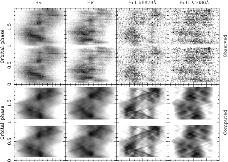
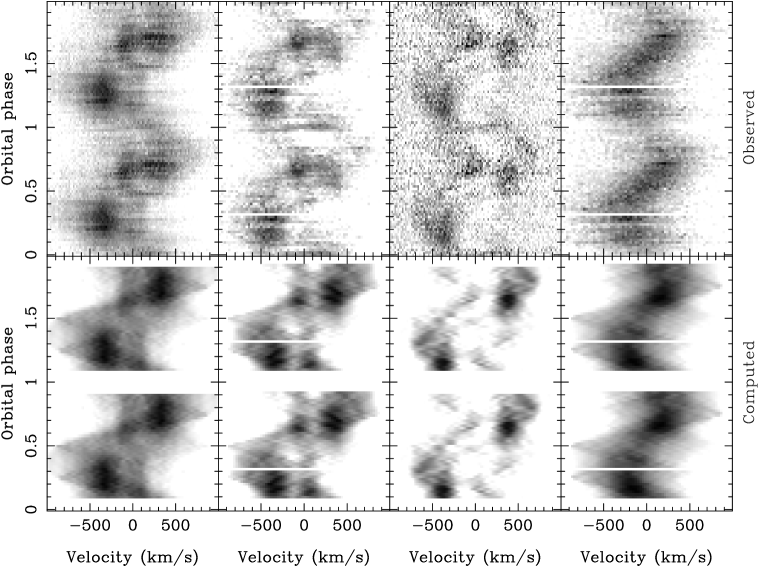
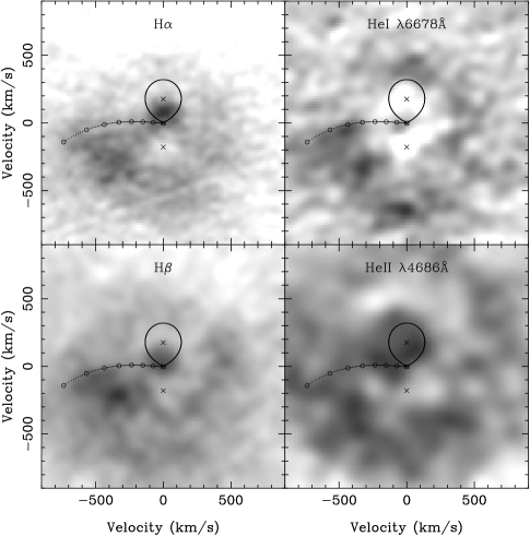
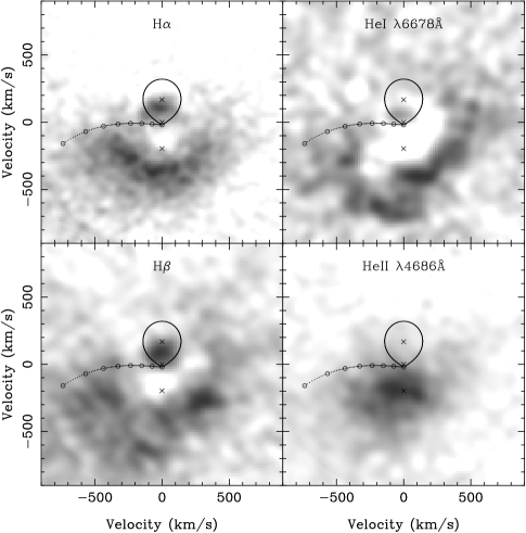
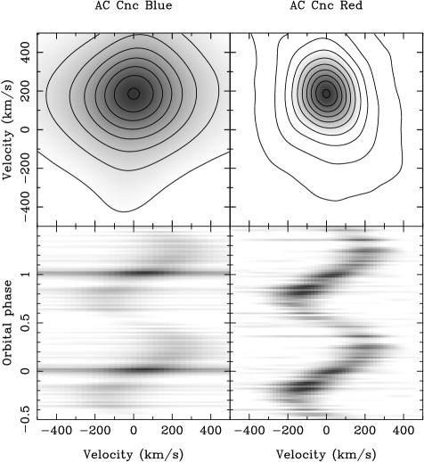
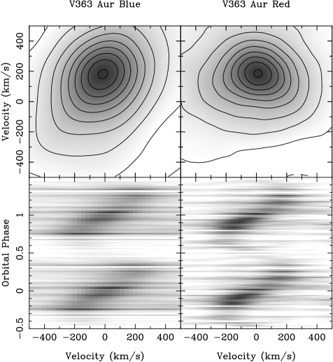
3.4 Trailed spectrum & Doppler Tomography
We subtracted polynomial fits to the continuum from the spectra and then rebinned the spectra onto a constant velocity–interval scale centred on the rest wavelength of the H, H, HeI 6678Å and HeII 4686Å lines. The data were then phase–binned into 50 bins, all of which were filled except for 1 empty bin at phase 0.31–0.33 in the blue V363 Aur data set. The trailed spectra of the lines are shown in the upper panels of Fig. 3 (a) and (b). We then constructed Doppler tomograms from the trailed spectra, a technique which maps the velocity–space distribution of the emission lines (e.g. ?). The Doppler maps are shown in Fig. 4 and trailed spectra reconstructed from the maps are presented in the lower panels of Fig. 3 (a) and (b).
The trailed spectra of AC Cnc show two clearly–defined components. The first is a high–amplitude S–wave with a semi–amplitude of 500km s-1, which crosses zero velocity from red to blue around phase 0.15. The emission is particularly noticable in H but can be seen in the other lines. This component appears in the Doppler map superimposed upon a ring of emission characteristic of an accretion disc at . This is what one would expect from the bright–spot, although it appears slightly downstream from where the computed gas stream joins the accretion disc, a trait also seen in other CVs (e.g. WZ Sge; ?). The second, lower–velocity component seen in the Balmer lines, seemingly in anti-phase with the higher–velocity component, shows up clearly in the Doppler maps as originating on the inner hemisphere of the secondary star. There is possibly another component visible in the HeI 6678Å line, which could be interpreted as the signature of a faint double–peaked accretion disc. All of the low–excitation lines exhibit the rotational disturbance expected from a high inclination accretion disc, but interestingly this is not seen in the HeII 4686Å line. These emission features are very similar to those seen in the novalike SW Sex (?).
The high–amplitude S–wave and the low–amplitude emission are also seen in V363 Aur, although the anti–phase sinusoid of the secondary is less well pronounced. The high–amplitude Balmer emission in the Doppler maps appears as a bright–spot downstream from where the gas stream meets the disc, as well as from the opposite side of the disc. There is clearly Balmer emission from the inner hemisphere of the secondary which is likely to be caused by irradiation by the accretion regions or white dwarf. The HeI trailed spectrum gives the visual impression of an absorption feature (moving at ) super–imposed on a high–velocity S–wave. The strange increase in Balmer line and HeI 6678Å emission at phase zero seen in the lightcurves is clearly visible in the trailed spectra. Possible explanations for this are given in Section 4. The high-excitation HeII 4686Å line is single-peaked throughout the orbit and the emission lies on the white dwarf centre of mass in the Doppler map.
| (a) AC Cnc |
 |
| (b) V363 Aur |
 |
|
3.5 Radial velocity of the white dwarf
We measured the radial velocities of the emission lines in AC Cnc and V363 Aur by applying the double–Gaussian method of ?, since this technique is sensitive mainly to the line wings and should therefore reflect the motion of the white dwarf with the highest reliability. We used Gaussians of widths 200, 300 and 400 km s-1 and varied their separation from 200 to 2500 km s-1. We then fitted
| (3) |
to each set of measurements, where is the radial velocity, the semi–amplitude, the orbital phase, and is the phase at which the radial velocity curve crosses from red to blue.
Examples of the radial velocity curves for AC Cnc and V363 Aur are shown in Fig. 5. The most striking feature of all of the radial velocity curves are the phase shifts, where the spectroscopic conjunction of each line occurs after photometric eclipse. This phase shift implies an emission line source trailing the accretion disc, such as a bright spot, and is a common feature of SW Sex stars (e.g. DW UMa, ?; V1315 Aql, ?; SW Sex, ?). There is clear evidence of rotational disturbance in the Balmer lines of AC Cnc, where the radial velocities measured just prior to eclipse are skewed to the red, and those measured after eclipse are skewed to the blue. This confirms the detection of a similar feature in the trailed spectra, and indicates that at least some of the emission must originate in the disc. We tried to measure white dwarf radial velocity () values from the emission lines in AC Cnc and V363 Aur using a diagnostic diagram (e.g. ?) and a light centres diagram (e.g. ?) but with no success. This is not surprising given that the Doppler maps (Fig. 4) show that the accretion disc does not dominate the emission in these systems. We conclude that the emission lines of AC Cnc and V363 Aur are unreliable indicators of the white dwarf radial velocity due to the phase shifts.


|
3.6 Radial velocity of the secondary star
The secondary star in both AC Cnc and V363 Aur is clearly visible in Fig. 1 through absorption lines of MgI, FeI and CaI. We compared regions of the spectra rich in absorption lines with a number of red dwarfs of spectral types G5V–M2V. A technique known as skew mapping was used to enhance the secondary features and obtain a radial velocity () measurement (see ? for a detailed critique of the method and ? for a successful application to BT Mon).
The first step was to shift the spectral type template stars to correct for their radial velocities. We then normalized each spectrum by dividing by a first–order polynomial fit, and then subtracting a higher order fit to the continuum. This ensures that line strength is preserved along the spectrum. The AC Cnc and V363 Aur spectra were normalized in the same way. The template spectra were artificially broadened to account for the orbital smearing of the CV spectra due to their exposure times () using the formula
| (4) |
(e.g. ?), and then by the rotational velocity of the secondary (). Estimated values of and were used in the first instance, before iterating to find the best–fitting values given in Section 3.10. Regions of the spectrum devoid of emission lines were then cross–correlated with each of the templates yielding a time series of cross–correlation functions (CCFs) for each template star. To produce the skew maps, these CCFs were back–projected in the same way as time–resolved spectra in standard Doppler tomography (?). If there is a detectable secondary star, we expect a peak at (0,) in the skew map. This can be repeated for each of the templates, and the final skew map is the one that gives the strongest peak.
The AC Cnc skew maps show well–defined peaks at 186 km s-1 – the skew map for the K2V template is shown in Fig. 6 together with the trailed CCFs and the regions used for the cross–correlation can be seen in Fig. 7. A systemic velocity of = 40 km s-1 was applied in order to shift the skew map peaks onto the = 0 axis. The value varies little with in practice, as in the back–projections (e.g. ?). We adopt = 40 5 km s-1 as the systemic velocity of the AC Cnc, in contrast to values of 122 km s-1 and 107 km s-1 found by ? using Balmer emission lines. Our adopted value of 186 3 km s-1 is derived from the best–fitting template (K2V), with the error incorporating the spread of values obtained by using different templates (see Table 4). The uncertainty also reflects the scatter in the radial velocity fits shown in Fig. 8. Note the remarkable agreement in the () values obtained from the red and blue data sets in Table 4. The small scatter in assures us that is robust, and the small scatter in around zero indicates that our assumed is correct.
The final V363 Aur skew maps for the G7V template (blue) and G5V template (red) and trailed CCFs are shown in Fig. 6, with the regions used for the cross–correlation marked in Fig. 7. For V363 Aur, the systemic velocity was less simple to determine, as the blue skew map suggested = –10 km s-1 and the red skew map gave = 10 km s-1. We can find no explanation for this discrepancy, so adopt a systemic velocity of = 0 10 km s-1. ? find systemic velocities ranging from 10 3 km s-1 for the HeII 4686Å line–wings to 35 3 km s-1 for the G-band absorption line. However, the peaks in the skew maps appear consistently at 184 km s-1. Our adopted value of = 184 5 km s-1 once again acknowledges the uncertainty in using different templates and the scatter in the radial velocity curves.
|
3.7 Rotational velocity and spectral type of the secondary star
In order to maximise the strength of the secondary features, we averaged the orbitally–corrected eclipse spectra of AC Cnc and V363 Aur. The spectral–type templates were broadened for smearing due to orbital motion as before and rotationally broadened by a range of velocities (50–240 km s-1). We then ran an optimal subtraction routine, which subtracts a constant times the normalized template spectrum from the normalized, orbitally–corrected CV spectrum, adjusting the constant to minimize the residual scatter between the spectra. The scatter is measured by carrying out the subtraction and then computing the between the residual spectrum and a smoothed version of itself. By finding the value of rotational broadening that minimizes the , we obtain an estimate of both and the spectral type of the secondary star. Note that the values of the template stars are much lower than the instrumental resolution, so do not affect our measurements of for the secondary star.
The value of obtained using this method varies depending on the spectral type template, the wavelength region for optimal subtraction, the amount of smoothing of the residual spectrum in the calculation of and the value of the limb–darkening coefficient used in the broadening procedure. The values of found from the G and K templates in the red and blue wavelength ranges, calculated using a limb–darkening coefficient of 0.5 and smoothed using a Gaussian of FWHM = 15km s-1, are listed in Table 4, together with the minimum . The optimal subtraction technique also tells us the value of the constant by which the template spectra were multiplied, which, for normalized spectra, is the fractional contribution of the secondary star to the total light in eclipse. These results are also summarised in Table 4.
For AC Cnc, the spectral types with the lowest values are G7V and K2V in blue and G9V in red, by no means offering a definitive answer. However, the fractional contribution of the secondary star must be less than one, ruling out a G type companion. By visually inspecting each of the spectra, we settle on a spectral type for the secondary star in AC Cnc of K2 1V. A plot of the AC Cnc average eclipse spectrum, a broadened template spectrum and the residual of the optimal subtraction is shown in Fig. 7. The analysis using a K2V template results in a measurement of 136 km s-1 in blue and 134 km s-1 in red, prompting us to adopt = 135 3 km s-1. This encompasses the value for all the G and early–mid K templates (except for the blue G5V) within 2. The error also reflects all of the other variations noted at the beginning of the previous paragraph. ? conclude that the secondary is a late G or early K star, not later than K3. We further limit this to an early K star, most likely K2V, agreeing with the studies of ? and ?. The results, however, conflict with the K5 estimate of ? based on colours. We find that, in eclipse, the secondary star in AC Cnc contributes 85 5 per cent of the total light in the blue and 74 19 per cent in the red, assuming a K2 1V spectral type.
For V363 Aur, the G7V template yields the lowest value in blue, and the G5V proves the best in red. Unfortunately, we did not record spectra of the G6V and G7V templates in red, so we can only conclude from this analysis and by visual inspection that V363 Aur has a secondary of G7 2V. The average is 147 5 km s-1 in the blue and 139 5 km s-1 in the red. We therefore adopt a compromise value of = 143 5 km s-1, encompassing all measurements for a G or early–mid K type secondary star. ? conclude that the spectral type is late G, and can be no later than K3, in agreement with this study. We do, however, rule out the estimate of a G0V star by ?. Using our adopted spectral type of G7 2V, we find that in eclipse the secondary contributes 25 3 per cent of the light in the blue and 45 8 per cent in the red.
At first glance, the fractional contributions of the secondary stars in the two systems during eclipse appear to be inconsistent. The K2 1V secondary star in AC Cnc contributes a larger fraction in blue than red, whereas the (intrinsically bluer) G7 2V secondary in V363 Aur contributes a smaller fraction. This can be explained by considering the different geometries of the two systems. In AC Cnc, almost all of the disc is obscured during eclipse, leaving only the redder outer disc uneclipsed. In V363 Aur, however, a large portion of the blue inner parts of the disc are still visible during eclipse (seen in Fig. 11), contributing significantly to the blue eclipse light. Outside eclipse, we measure the fractional contribution of the secondary star in AC Cnc to be 19 2 per cent in blue and 40 11 per cent in red. Similar values are found for V363 Aur with out-of-eclipse contributions of 19 4 per cent in blue and 35 7 per cent in red.
 |
 |
| (a) AC Cnc | ||||||||||||
| Templates | min | min | Fractional | Fractional | () from | () from | ||||||
| (blue) | at min | (red) | at min | contribution | contribution | skew map | skew map | |||||
| (blue) | (red) | of secondary | of secondary | (blue) | (red) | |||||||
| km s-1 | km s-1 | (blue) | (red) | km s-1 | km s-1 | |||||||
| G5V | 1.081 | 142 | 1.106 | 136 | 1.24 | 0.03 | 1.13 | 0.10 | (3, | 187) | (–4, | 185) |
| G6V | 1.066 | 140 | – | – | 1.15 | 0.03 | – | (3, | 186) | – | ||
| G7V | 1.038 | 140 | – | – | 1.18 | 0.03 | – | (–2, | 185) | – | ||
| G8V | 1.046 | 141 | 1.100 | 137 | 1.20 | 0.03 | 1.22 | 0.11 | (–1, | 186) | (–4, | 187) |
| G9V | 1.080 | 139 | 1.097 | 136 | 1.19 | 0.03 | 1.37 | 0.12 | (3, | 186) | (–4, | 186) |
| K0V | 1.043 | 138 | 1.107 | 135 | 1.04 | 0.02 | 0.99 | 0.09 | (1, | 185) | (–4, | 187) |
| K1V | – | – | 1.112 | 134 | – | 0.93 | 0.08 | – | (–9, | 186) | ||
| K2V | 1.038 | 136 | 1.112 | 134 | 0.85 | 0.02 | 0.74 | 0.07 | (0, | 187) | (0, | 185) |
| K3V | 1.127 | 134 | – | – | 0.82 | 0.02 | – | (–2, | 186) | – | ||
| K4V | 1.406 | 138 | 1.137 | 131 | 0.62 | 0.02 | 0.46 | 0.04 | (3, | 189) | (–2, | 185) |
| K5V | 1.288 | 135 | 1.128 | 131 | 0.67 | 0.02 | 0.56 | 0.05 | (0, | 187) | (–10, | 186) |
| K7V | 1.319 | 136 | 1.125 | 130 | 0.65 | 0.02 | 0.55 | 0.05 | (4, | 186) | (–3, | 186) |
| K8V | 1.437 | 136 | 1.138 | 129 | 0.63 | 0.02 | 0.50 | 0.05 | (0, | 188) | (–4, | 184) |
| (b) V363 Aur | ||||||||||||
| G5V | 1.081 | 148 | 1.119 | 139 | 0.25 | 0.01 | 0.43 | 0.07 | (–7, | 184) | (10, | 185) |
| G6V | 1.081 | 146 | – | – | 0.25 | 0.01 | – | (–8, | 184) | – | ||
| G7V | 1.054 | 148 | – | – | 0.27 | 0.01 | – | (–13, | 181) | – | ||
| G8V | 1.068 | 148 | 1.122 | 138 | 0.26 | 0.01 | 0.46 | 0.08 | (–11, | 184) | (12, | 184) |
| G9V | 1.098 | 143 | 1.120 | 140 | 0.24 | 0.01 | 0.52 | 0.09 | (–4, | 183) | (13, | 185) |
| K0V | 1.086 | 143 | 1.126 | 140 | 0.21 | 0.01 | 0.37 | 0.07 | (–6, | 185) | (15, | 184) |
| K1V | – | – | 1.120 | 138 | – | 0.37 | 0.06 | – | (7, | 189) | ||
| K2V | 1.107 | 142 | 1.136 | 146 | 0.17 | 0.01 | 0.29 | 0.06 | (–9, | 186) | (13, | 185) |
| K3V | 1.150 | 139 | – | – | 0.17 | 0.01 | – | (–10, | 184) | – | ||
| K4V | 1.294 | 134 | 1.140 | 146 | 0.10 | 0.01 | 0.19 | 0.04 | (0, | 191) | (9, | 186) |
| K5V | 1.234 | 134 | 1.132 | 141 | 0.11 | 0.01 | 0.24 | 0.04 | (5, | 188) | (8, | 188) |
| K7V | 1.252 | 132 | 1.134 | 145 | 0.11 | 0.01 | 0.23 | 0.04 | (0, | 191) | (12, | 187) |
| K8V | 1.297 | 134 | 1.138 | 148 | 0.10 | 0.01 | 0.22 | 0.04 | (–4, | 188) | (8, | 187) |
3.8 The Correction
The irradiation of the secondary stars in CVs by the emission regions around the white dwarf and the bright spot has been shown to influence the measured (e.g. ? and ?). For example, if absorption lines are quenched on the irradiated side of the secondary, the centre of light will be shifted towards the back of the star. The measured will then be larger than the true (dynamical) value.
We must now determine whether the secondary stars in AC Cnc and V363 Aur are irradiated, which can be observationally tested in two ways. Firstly, the rotationally broadened line profile would be distorted if there was a non–uniform absorption distribution across the surface of the secondary star (?). This would result in a non–sinusoidal radial velocity curve. Secondly, one would expect a depletion of absorption line flux from the secondary star at phase 0.5, where the quenched inner–hemisphere is pointed towards the observer (e.g. ?). We applied these tests to the AC Cnc and V363 Aur data.
The secondary star radial velocity curves were produced by cross–correlating the CV spectra with the best–fitting smeared and broadened template spectra as described in Section 3.6. This time the cross–correlation peaks were plotted against phase to produce the radial velocity curves shown in the lower panels of Fig. 8. The radial velocity curves of both AC Cnc and V363 Aur are clearly eccentric in comparison to the sinusoidal fits represented by the thin solid lines.
The variation of secondary star absorption line flux with phase for AC Cnc and V363 Aur is shown in the top panels of Fig. 8. These lightcurves were produced by optimally subtracting the smeared and rotationally broadened best–fitting template from the individual CV spectra (with the secondary radial velocity shifted out) as described in Section 3.7. This time, however, the spectra were continuum subtracted rather than normalised to ensure that the measurements were not affected by a fluctuating disc brightness. The constants produced by the optimal subtraction are secondary star absorption line fluxes, correct relative to each other, but not in an absolute sense. The dashed lines super–imposed on the lightcurves represent the variation of flux with phase for a Roche lobe with a uniform absorption distribution. The sinusoidal nature is the result of the changing projected area of the Roche lobe through the orbit. The lightcurves of AC Cnc and V363 Aur exhibit a drop in flux at phase 0.5 in comparison with the uniform Roche lobe.
These two pieces of evidence, as well as the observed Balmer emission from the inner hemisphere of the secondary stars seen in Figs. 3 and 4, and the weakening of the CCFs around phase 0.5 seen in Fig. 6 suggest that the secondary stars in AC Cnc and V363 Aur are indeed irradiated and we must correct the values accordingly.
It is possible to correct for the effects of irradiation by modelling the secondary star absorption line flux distribution. In our model, we divided the secondary Roche lobe into 40 vertical slices of equal width. We then produced a series of model lightcurves, varying the numbers of slices omitted from the inner hemisphere of the secondary which contribute to the total flux. The model lightcurves were then scaled to match the observed data, and the best–fitting model found by measuring the between the two. In all models, we used a gravity–darkening parameter and limb–darkening coefficient (e.g. ?). There is evidence for a secondary eclipse in both systems, so we have omitted points around phase 0.5 from the fits. (We tried a model which included an accretion disc to reproduce the secondary eclipse, but the results were exactly the same as omitting the points.) Once the best–fitting lightcurve was found, we produced fake CV spectra from the models, which were cross-correlated with a fake template star to produce a synthetic radial velocity curve. In the first instance, the synthetic curve mimicked the non-sinusoidal nature of the observed data, but with a larger semi–amplitude. This was expected, as the model input parameters used the uncorrected derived in Section 3.10. We then lowered and repeated the process, until the semi–amplitude of the model and observed radial velocity curves were in agreement, each time checking the lightcurve models for goodness of fit. The resulting was then adopted as the real (or dynamical) value.
For AC Cnc, the best–fitting model lightcurve was produced by omitting 8 slices when fitting both the blue and red data. The model lightcurves omitting 7, 8 and 9 slices are shown by the solid lines in Fig. 8. Our final model, which has an input of 176 km s-1, produces the radial velocity curve shown as the thick solid line in Fig. 8. There is excellent agreement between this and the observed data. The best–fitting lightcurve models for V363 Aur have 10 slices omitted in blue and 8 slices in red. Model lightcurves omitting 9, 10 and 11 slices in blue and 7, 8 and 9 slices in red are once again shown as solid lines in Fig. 8. The red data are very noisy, so we used the blue data to obtain a corrected of 168 km s-1. The model with this input value has the radial velocity curve plotted as the thick solid line in Fig. 8. It should be noted that if gravity–darkening and limb–darkening are neglected, the best fit lightcurves remain the same in all cases, and produce values which are 3 km s-1 lower.
The points around primary eclipse in the blue lightcurve of AC Cnc were also omitted from the above fit, as they show a very sharp decrease in flux. Although some of this can be attributed to the reduced projected area of the secondary at phase 0, the feature is too sharp and too deep for this to be the only explanation. It is likely that this feature is an artefact of the slit–loss correction procedure, where –band photometry has been used to correct secondary features which actually lie closer to the –band. Because the –band eclipse is deeper than the –band eclipse, we get a residual sharp dip in the secondary star flux at phase 0. There is no corresponding dip in the red data, as the photometry and spectroscopy wavelengths are closely matched. There is no corresponding dip in flux at phase 0 in the blue V363 Aur data, even though both objects have been reduced in the same way. We believe this is because the –band eclipse depth is approximately the same as the –band eclipse depth in V363 Aur.
In summary, we correct the of AC Cnc from 186 km s-1 to 176 km s-1 and the of V363 Aur from 184 km s-1 to 168 km s-1.
| (a) AC Cnc |
 |
| (b) V363 Aur |
 |
3.9 The distances to AC Cnc and V363 Aur
By finding the apparent magnitude of the secondary star from its contribution to the total light during eclipse, and estimating its absolute magnitude, we can calculate the distance () to each system using the equation:
| (5) |
where is the visual interstellar extinction in magnitudes per kpc.
There are a number of ways of estimating the absolute magnitude of the secondary star, assuming it is on the main sequence (e.g. ?; ?; ?). The distance estimates given below take into account all of these techniques.
Another method of finding the distance is to determine the angular diameter of the secondary star from the observed flux and a surface brightness calibration that we derive from the Barnes–Evans relation (?),
| (6) |
where and are the unreddened magnitude and colour of the secondary star, and is the stellar angular diameter in arc milliseconds.
3.9.1 AC Cnc
During the eclipse phases given in Section 3.7, the average apparent magnitude of AC Cnc is = 14.7 0.1, of which the secondary contributes 74 19 per cent, and = 15.9 0.1, of which the secondary star contributes 85 5 per cent. The apparent magnitude of the secondary is therefore = 15.0 0.3 and = 16.1 0.1. Using typical and values for an early K star from ?, we arrive at an apparent magnitude of 15.5 0.3. We adopt an absolute magnitude of as an average of the various methods referenced in the previous paragraph. Assuming zero interstellar extinction (?), the distance to AC Cnc is 550 150 pc.
Using the Barnes–Evans relation with a value typical of an early K star (0.74 0.10; ?), the value of 15.5 0.3 found above and the radius of the secondary star derived in Section 3.10, we obtain a distance of 750 250 pc.
Published estimates of the distance to AC Cnc agree with our calculated values. ? calculates a distance of 480 pc assuming a K5 secondary star. ? derives a value of 400 pc by combining an –H equivalent–width relationship, properties of the secondary and the continuum shape of the spectrum. ? calculates a distance of 800 pc using the secondary star characteristics from ? and ? concludes = 500 100 pc, again estimating the secondary star properties.
3.9.2 V363 Aur
The average apparent magnitude of V363 Aur during the eclipse phases quoted in Section 3.7 is = 14.8 0.1 and = 13.9 0.1, of which the G7 2V secondary star contributes 25 3 per cent and 45 8 per cent, respectively. This corresponds to an apparent magnitude of the secondary star of = 16.3 0.2, = 14.8 0.2 and, assuming typical and values for a G7 2V star (?), we calculate = 15.4 0.2. There is evidence of interstellar absorption in the average spectrum (Fig. 1), suggesting that it is important to take extinction into account. ? give a value of = 0.3, although the UV spectrum used was underexposed and noisy. ?, however, finds no extinction to V363 Aur, a result contradicted by measurements of ?, who measure = 0.1. We adopt this value, which results in (?). We use as an average absolute magnitude of the G7 2V star secondary star in V363 Aur, which results in a distance of 700 250 pc.
Using the Barnes–Evans relation with a value typical of a mid–late G star (0.56 0.1; ?), a value of 15.1 0.2 assuming extinction to be 0.3 mag and the radius of the secondary star derived in Section 3.10, we obtain a distance of 1000 250 pc.
? estimate a distance to V363 Aur of 900 pc assuming a G0 dwarf secondary. ? derives an uncertain value of 1000 pc from the –H equivalent–width relationship, interstellar absorption and the continuum shape of the spectrum. In his compilation of distances, ? gives a distance of 1100 pc from disc properties, 900–1300 pc from red star spectrophotometry and 450pc from the infrared properties of the secondary. ? calculate a distance of 530 pc from a black body fit to the spectrum of the central part of the disc and 720 pc using a value for the fractional contribution of the secondary.
3.10 System Parameters
Using the and values found in Sections 3.7 and 3.8 in conjunction with the period determined in Section 3.1 and a measurement of the eclipse full–width at half depth (), we can calculate accurate system parameters for AC Cnc and V363 Aur.
In order to determine , we estimated the flux out of eclipse (the principal source of error) and at eclipse minimum, and then measured the full–width of the eclipse half-way between these points. The eclipse full–width at half-depth was measured to be = 0.096 0.002 for AC Cnc and 0.063 0.002 for V363 Aur from the and –band lightcurves in Fig. 2.
We have opted for a Monte Carlo approach similar to ? to calculate the system parameters and their errors. For a given set of , , and , the other system parameters are calculated as follows.
can be estimated because we know that the secondary star fills its Roche lobe (as there is an accretion disc present and hence mass transfer). is the equatorial radius of the secondary star and is the binary separation. We used Eggleton’s formula (?) which gives the volume-equivalent radius of the Roche lobe to better than 1 per cent, which is close to the equatorial radius of the secondary star as seen during eclipse,
| (7) |
The secondary star rotates synchronously with the orbital motion, so we can combine and , to get
| (8) |
By considering the geometry of a point eclipse by a spherical body (e.g. ?), the radius of the secondary can be shown to be
| (9) |
which, using the value of obtained using equations 7 and 8, allows us to calculate the inclination () of the system. The geometry of a disc eclipse can be approximated to a point eclipse if the light distribution around the white dwarf is axi–symmetric (e.g. ?). This approximation is justified given the symmetry of the primary eclipses in the photometry light curves (Figure 2). Kepler’s Third Law gives us
| (10) |
which, with the values of and calculated using equations 7, 8 and 9, gives the mass of the primary star. The mass of the secondary star can then be obtained using
| (11) |
The radius of the secondary star is obtained from the equation
| (12) |
(e.g. ?) and the separation of the components, , is calculated from equations 8 and 12 with and now known.
The Monte Carlo simulation takes 10 000 values of , , and (the error on the period is deemed to be negligible in comparison to the errors on , , and ), treating each as being normally distributed about their measured values with standard deviations equal to the errors on the measurements. We then calculate the masses of the components, the inclination of the system, the radius of the secondary star, and the separation of the components, as outlined above, omitting (, , ) triplets which are inconsistent with . Each accepted pair is then plotted as a point in Figure 9, and the masses and their errors are computed from the mean and standard deviation of the distribution of these pairs.
In the case of AC Cnc, we find that and ; for V363 Aur we find and . The values of all the system parameters deduced from the Monte Carlo computation are listed in Table 5, including –corrected and non –corrected values for comparison.
We computed the radius of the accretion discs in AC Cnc and V363 Aur using the geometric method outlined in ?. The phase half-width of eclipse at maximum intensity was found in Section 3.3 to be for AC Cnc and for V363 Aur. Combining with and derived above produces an accretion disc radius () in terms of the volume radius of the primary’s Roche lobe (). We find accretion disc radii of and for AC Cnc and V363 Aur, respectively, which are lower than those quoted by ?, but consistent within the errors; AC Cnc: , V363 Aur: .
The empirical relation obtained by ? between mass and radius for the secondary stars in CVs is given by,
| (13) |
This predicts that if the secondary stars in AC Cnc and V363 Aur are on the main-sequence, they should have radii of 0.78 and 1.05, respectively. These values agree with our measured values of 0.83 0.03 and 0.97 0.04 to within the errors. ? gives and for a K2 dwarf and and for a G5 dwarf, also in agreement with our measured values. We conclude that the secondaries in AC Cnc and V363 Aur are similar to main–sequence stars.


|
| Parameter | AC Cnc | V363 Aur | ||||||||||
| ——————————————————————————————————————————— | ||||||||||||
| Measured | Monte Carlo | –corrected | Measured | Monte Carlo | –corrected | |||||||
| Value | Value | Value | Value | Value | Value | |||||||
| (d) | 0.30047747 | 0.30047747 | 0.32124187 | 0.32124187 | ||||||||
| (km s-1) | 186 | 3 | 186 | 3 | 176 | 3 | 184 | 5 | 184 | 5 | 168 | 5 |
| (km s-1) | 135 | 3 | 135 | 3 | 135 | 3 | 143 | 5 | 143 | 5 | 143 | 5 |
| 0.096 | 0.003 | 0.096 | 0.003 | 0.096 | 0.003 | 0.063 | 0.002 | 0.063 | 0.002 | 0.063 | 0.002 | |
| 0.94 | 0.04 | 1.02 | 0.04 | 1.04 | 0.06 | 1.17 | 0.07 | |||||
| 76.3 | 0.8 | 75.6 | 0.7 | 70.5 | 0.4 | 69.7 | 0.4 | |||||
| (km s-1) | 175 | 6 | 179 | 6 | 190 | 9 | 196 | 9 | ||||
| 0.82 | 0.04 | 0.76 | 0.03 | 1.03 | 0.07 | 0.90 | 0.06 | |||||
| 0.78 | 0.05 | 0.77 | 0.05 | 1.06 | 0.11 | 1.06 | 0.11 | |||||
| 0.82 | 0.02 | 0.83 | 0.02 | 0.96 | 0.04 | 0.97 | 0.04 | |||||
| 2.21 | 0.04 | 2.18 | 0.04 | 2.52 | 0.07 | 2.47 | 0.07 | |||||
| (pc) | 550 | 150 | 700 | 250 | ||||||||
| (pc) | 750 | 250 | 1000 | 250 | ||||||||
| Spectral type | K2 | 1 V | G7 | 2 V | ||||||||
| of secondary | ||||||||||||
| 0.09 | 0.01 | 0.078 | 0.005 | |||||||||
| 0.61 | 0.14 | 0.71 | 0.17 | |||||||||
4 Discussion
4.1 Are AC Cnc and V363 Aur SW Sex stars?
The SW Sex stars are a sub–class of NLs which have peculiar spectral properties – see ? and references therein for a summary of the current models. Most SW Sex stars share the following properties (e.g. ?):
-
1.
They are usually high–inclination, eclipsing systems.
-
2.
Their spectra exhibit single–peaked emission lines rather than the double–peaked lines expected from near edge–on discs.
-
3.
The Balmer and HeI emission lines usually contain transient absorption cores, especially around photometric phase 0.5.
-
4.
They have high levels of excitation, with HeII 4686Å emission often comparable in strength to H.
-
5.
The low–excitation lines (Balmer and HeI) exhibit shallow or absent eclipses.
-
6.
High velocity S–waves are often seen in the trailed spectra.
-
7.
The emission–line radial velocity curves show large phase shifts between spectroscopic conjunction and photometric mid–eclipse.
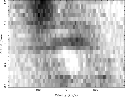
AC Cnc and V363 Aur show many of the features described above. V363 Aur shows all of the features, so must be considered a definite SW Sex star. AC Cnc does show high excitation features, but not to the extent of V363 Aur. Transient absorption features are seen in low–excitation lines of both systems. An interesting absorption feature also occurs around phase 0 in V363 Aur, which deserves further discussion.
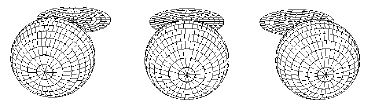
The low–excitation emission lines of V363 Aur show the broad primary eclipse expected from a gradual obscuration of the accretion disc by the secondary (see Fig.2). Around phase 0, however, there is a sharp increase in Balmer line emission followed by a rapid decrease. The feature comes and goes too rapidly to be attributable to a permanent emission source on the back of the secondary star. We suggest that this increase in flux can be explained by the eclipse of an optically thick region at the centre of the disc. The eclipse of this region, which would have an absorption line spectrum, would result in an overall increase in the line flux at the phases observed. Fig. 10 is the trailed spectrum of H magnified to show the effect more clearly. The blue wing of the line increases in flux first, in agreement with an eclipse of the centre of the disc. Fig. 11 is a reconstruction of V363 Aur using the –corrected system parameters listed in Fig. 5. The left–hand diagram shows the system just before the increase in flux at phase 0.97, where the centre of the disc is just about to be eclipsed by the secondary. In the central diagram, the centre of the disc is eclipsed, corresponding to the brief rise in line flux. The right–hand diagram shows the system at phase 1.03, when the centre of the disc comes out of eclipse, and the line flux drops again. The short timescale of this feature is explained by the grazing nature of the eclipse of the optically thick region at the centre of the disc. This model could also account for the behaviour of other SW Sex stars where the Balmer lines show only a shallow eclipse compared to the continuum. ? and ? suggest a similar explanation for SW Sex. The latter authors invoked an optically thick absorption–line source coincident with the bright spot, similar to that of a late B or early A–type star.
4.2 Mass Transfer Stability

The mass ratio () of a CV is of great significance, as it governs the properties of mass transfer from the secondary to the white dwarf primary. This in turn governs the evolution and behaviour of the system.
The secondary star has two timescales on which it responds to mass loss. Firstly, the star returns to hydrostatic equilibrium on a dynamical timescale, which is the sound–crossing time of the region affected. Secondly, on a longer timescale, the star settles into a new thermal equilibrium configuration. The second timescale a star responds on is therefore the thermal, or Kelvin-Helmholtz, timescale.
The two timescales upon which the secondary responds to mass loss leads to two types of mass transfer instability. If, upon mass loss, the dynamical response of the secondary is to expand relative to the Roche lobe, mass transfer is dynamically unstable and mass transfer proceeds on the dynamical timescale. ? made an analytic fit to the models of ? to give the limit of dynamically stable mass loss, plotted as the solid line in Fig. 12. Dynamically stable mass transfer can occur if the CV lies below this line. This limit is important for low mass secondary stars (), as they have significant convective envelopes that tend to expand adiabatically in response to mass loss (?).
Thermally unstable mass transfer is possible if the dynamic response of the star to mass loss is to shrink relative to its Roche lobe (i.e. mass transfer is dynamically stable). This occurs at high donor masses () when the star has a negligible convective envelope and its adiabatic response to mass loss is to shrink (e.g. ?; ?). Mass transfer then initially breaks contact and the star begins to settle into its new thermal equilibrium configuration. If the star’s thermal equilibrium radius is now bigger than the Roche lobe, mass transfer is again unstable, but proceeds on the slower, thermal timescale. The limit of thermally stable mass transfer can be found by differentiating the main–sequence mass–radius relationship given in ?. Thermally stable mass transfer can occur if the CV appears below the dotted line plotted in Fig. 12.
Most CVs on the plot fall below both curves, implying that mass transfer is dynamically and thermally stable, as expected (the mass transfer rates observed in CVs are too low for unstable mass transfer to be occurring). An exception is DX And, which appears to be dynamically unstable. This is, of course, not possible; a system undergoing dynamical mass transfer would rapidly form a common envelope. A solution is found in the fact that DX And has an evolved secondary star (?); the dynamical and thermal solutions plotted on Fig. 12 are for ZAMS stars, so cannot be applied to evolved stars.
The previous study of the masses of AC Cnc by ? found a value of 1.24 0.08, close to the limit for thermally stable mass transfer. In this study, we find a lower value of = 1.02 0.04, placing it well within the theoretical limit. In the case of V363 Aur, we find a higher value of 1.17 0.07 than the value of = 0.90 0.10 quoted by ?, but it is still within the stability limit. The mass ratios found in this paper therefore place AC Cnc and V363 Aur within the region allowed by the theoretical constraints for stable mass transfer.
Acknowledgements
We thank N. Samus and E. Zhang for providing eclipse timings of AC Cnc, and Homer Giannakis for help in reducing the photometry. We are indebted to Tom Marsh for the use of his software packages PAMELA and MOLLY, and we thank Uli Kolb, Stuart Littlefair and Tariq Shabaz for useful discussions. We also thank the referee, Robert Smith, for his careful reading of the manuscript and suggestions for improvements. TDT and MJS are supported by PPARC studentships; CAW is supported by PPARC grant number PPA/G/S/2000/00598. DS acknowledges a Smithsonian Astrophysical Observatory Clay Fellowship. The INT and JKT are operated on the island of La Palma by the Isaac Newton Group in the Spanish Observatorio del Roque de los Muchachos of the Instituto de Astrofisica de Canarias.
References
- Barnes & Evans (1976) Barnes T. G., Evans D. S., 1976, MNRAS, 174, 489
- Berriman (1987) Berriman G., 1987, A&AS, 68, 41
- Davey & Smith (1992) Davey S. C., Smith R. C., 1992, MNRAS, 257, 476
- de Kool (1992) de Kool M., 1992, AA, 261, 188
- Dhillon, Jones & Marsh (1994) Dhillon V. S., Jones D. H. P., Marsh T. R., 1994, MNRAS, 266, 859
- Dhillon, Marsh & Jones (1991) Dhillon V. S., Marsh T. R., Jones D. H. P., 1991, MNRAS, 252, 342
- Dhillon, Marsh & Jones (1997) Dhillon V. S., Marsh T. R., Jones D. H. P., 1997, MNRAS, 291, 694
- Dhillon (1990) Dhillon V. S., 1990, D. Phil thesis, University of Sussex
- Downes (1982) Downes R. A., 1982, PASP, 94, 950
- Drew, Jones & Woods (1993) Drew J. E., Jones D. H. P., Woods J. A., 1993, MNRAS, 260, 803
- Eggleton (1983) Eggleton P. P., 1983, ApJ, 268, 368
- Friend et al. (1990) Friend M. T., Martin J. S., Smith R. C., Jones D. H. P., 1990, MNRAS, 246, 637
- Gray (1992) Gray D. F., 1992, The Observation and Analysis of Stellar Photospheres. Cambridge University Press, Cambridge
- Groot, Rutten & van Paradijs (2001) Groot P. J., Rutten R. G. M., van Paradijs J., 2001, AA, 368, 183
- Harrop-Allin & Warner (1996) Harrop-Allin M. K., Warner B., 1996, MNRAS, 279, 219
- Hellier (2000) Hellier C., 2000, New Astronomy Reviews, 44, 131
- Helmer & Morrison (1985) Helmer L., Morrison L. V., 1985, Vistas in Astronomy, 28, 515
- Henden & Honeycutt (1995) Henden A. A., Honeycutt R. K., 1995, PASP, 107, 324
- Hjellming (1989) Hjellming M. S., 1989, PhD thesis, University of Illinois
- Hoard et al. (2003) Hoard D. W., Szkody P., Froning C. S., Long K. S., Knigge C., 2003, AJ, 126, 2473
- Horne, Lanning & Gomer (1982) Horne K., Lanning H. H., Gomer R. H., 1982, ApJ, 252, 681
- Horne, Welsh & Wade (1993) Horne K., Welsh W. F., Wade R. A., 1993, ApJ, 410, 357
- Knigge et al. (2000) Knigge C., Long K. S., Hoard D. W., Szkody P., Dhillon V. S., 2000, ApJ, 539, L49
- Kurochkin & Shugarov (1980) Kurochkin N. E., Shugarov S. Y., 1980, Astron. Tsirk, No. 1114
- la Dous (1991) la Dous C., 1991, AA, 252, 100
- Lanning (1973) Lanning H., 1973, PASP, 85, 70
- Margon & Downes (1981) Margon B., Downes R., 1981, AJ, 86, 747
- Marsh & Horne (1988) Marsh T. R., Horne K., 1988, MNRAS, 235, 269
- Marsh (1988) Marsh T. R., 1988, MNRAS, 231, 1117
- Marsh (2001) Marsh T. R., 2001, in Boffin H., Steeghs D., Cuypers J., eds, Proceedings of the International Workshop on Astro-tomography, Brussels, July 2000. Springer-Verlag Lecture Notes in Physics, Dusseldorf, p. 1
- North et al. (2000) North R. C., Marsh T. R., Moran C. K. J., Kolb U., Smith R. C., Stehle R., 2000, MNRAS, 313, 383
- Okazaki, Kitamura & Yamasaki (1982) Okazaki A., Kitamura M., Yamasaki A., 1982, PASP, 94, 162
- Patterson (1984) Patterson J., 1984, ApJS, 54, 443
- Politano (1996) Politano M., 1996, ApJ, 465, 338
- Rutten, van Paradijs & Tinbergen (1992) Rutten R. G. M., van Paradijs J., Tinbergen J., 1992, AA, 260, 213
- Scheffler (1982) Scheffler H. in Schaifers K., Voigt H. H., eds, Landolt–Börnstein Numerical Data and Functional Relationships in Science and Technology, New Series, Group VI, Vol. 2, Subvol. c, p. 47, Springer Verlag, Heidelberg, 1982
- Schlegel, Honeycutt & Kaitchuck (1986) Schlegel E. M., Honeycutt R. K., Kaitchuck R. H., 1986, ApJ, 307, 760
- Schlegel, Kaitchuck & Honeycutt (1984) Schlegel E. M., Kaitchuck R. H., Honeycutt R. K., 1984, ApJ, 280, 235
- Schneider & Young (1980) Schneider D. P., Young P. J., 1980, ApJ, 238, 946
- Shafter, Hessman & Zhang (1988) Shafter A. W., Hessman F. V., Zhang E. H., 1988, ApJ, 327, 248
- Shafter, Szkody & Thorstensen (1986) Shafter A. W., Szkody P., Thorstensen J. R., 1986, ApJ, 308, 765
- Shugarov (1981) Shugarov S. Y., 1981, Sov. Astron., 25, 332
- Smith & Dhillon (1998) Smith D. A., Dhillon V. S., 1998, MNRAS, 301, 767
- Smith, Dhillon & Marsh (1998) Smith D. A., Dhillon V. S., Marsh T. R., 1998, MNRAS, 296, 465
- Spruit & Rutten (1998) Spruit H. C., Rutten R. G. M., 1998, MNRAS, 299, 768
- Szkody & Crosa (1981) Szkody P., Crosa L., 1981, ApJ, 251, 620
- Thoroughgood et al. (2001) Thoroughgood T. D., Dhillon V. S., Littlefair S. P., Marsh T. R., Smith D. A., 2001, MNRAS, 327, 1323
- Vande Putte et al. (2003) Vande Putte D., Smith R. C., Hawkins N. A., Martin J. S., 2003, MNRAS, 342, 151
- Wade & Horne (1988) Wade R. A., Horne K., 1988, ApJ, 324, 411
- Warner (1987) Warner B., 1987, MNRAS, 227, 23
- Warner (1995a) Warner B., 1995a, Cataclysmic Variable Stars. Cambridge University Press, Cambridge
- Warner (1995b) Warner B., 1995b, Ap&SS, 232, 89
- Watson & Dhillon (2001) Watson C. A., Dhillon V. S., 2001, MNRAS, 326, 67
- Watson et al. (2003) Watson C. A., Dhillon V. S., Rutten R. G. M., Schwope A. D., 2003, MNRAS, 341, 129
- Yamasaki, Okazaki & Kitamura (1983) Yamasaki A., Okazaki A., Kitamura M., 1983, Publ. Astron. Soc. Japan, 35, 423
- Zhang (1987) Zhang E., 1987, Acta Astrophysica Sinica, 7, 245