INJE-TP-04-04

astro-ph/0406387

Test of patch cosmology with WMAP

Kyong Hee Kim¹ and Yun Soo Myung^1,2

¹Relativity Research Center and School of Computer Aided School, Inje University Gimhae 621-749, Korea
²Institute of Theoretical Science, University of Oregon, Eugene, OR 97403-5203, USA

We calculate the power spectrum, spectral index, and running spectral index for inflationary patch cosmology arisen from Gauss-Bonnet braneworld scenario using the Mukhanov equation. This patch cosmology consists of Gauss-Bonnet(GB), Randall-Sundrum (RS-II), and four dimensional (4D) cosmological models. There exist several modifications in higher order calculations. However, taking the power-law inflation by choosing different potentials depending on the model, there exist minor changes up to second order corrections. Since second order corrections are rather small in the slow-roll limit, we could not choose a desired power-law model which explains the WMAP data. Finally we discuss the reliability of high order calculations based on the Mukhanov equation by comparing the perturbed equation including 5D metric perturbations. It turns out that first order corrections are reliable, while second order corrections are not proved to be reliable.

1 Introduction

There has been much interest in the phenomenon of localization of gravity proposed by Randall and Sundrum[1]. They assumed a single positive tension 3-brane and a negative bulk cosmological constant in the five dimensional (5D) spacetime. They obtained a localized gravity on the brane by fine-tuning the tension to the cosmological constant. Recently, several authors studied cosmological implications of brane world scenario. The brane cosmology contains some important deviations from the Friedmann-Robertson-Walker (FRW) cosmology[2, 3]. The Friedmann equation is modified at high energy significantly.

On the other hand, it is generally accepted that curvature perturbations produced during inflation are the origin of anisotropies for CMB and inhomogeneities for galaxy formation and other large-scale structures. The WMAP, SDSS and Lyman alpha put forward constraints on cosmological models and confirm the emerging standard model of cosmology, a flat $\Lambda$-dominated universe seeded by scale-invariant adiabatic gaussian fluctuations[4, 5, 6, 7, 8]. In other words, these results coincide with theoretical predictions of the slow-roll inflation based on general relativity and a single inflaton. Further, the future experiments of Planck will be able to place more stringent constraints on running spectral index than those of WMAP and Lyman alpha.

If the brane inflation occurs, one expects that it gives us different results in the high-energy regime. Maartens et al.[9] have described the inflationary perturbation in the brane cosmology using the slow-roll approximation and potential slow-roll parameters. Liddle and Taylor[10] have shown that in the slow-roll approximation, the scalar perturbations alone cannot be used to distinguish between the standard and brane inflations. Ramirez and Liddle[11] have studied the same issue using the slow-roll approximation with Hubble slow-roll parameters. They found that the first-order correction to the brane cosmology is of a similar size to that in the standard cosmology. Also Tsujikawa and Liddle[12] have investigated observational constraints on the brane inflation from CMB anisotropies by introducing the large-field, small-field, and hybrid models. Unfortunately, in the slow-roll approximation[13], there is no significant change in the power spectrum between the standard and brane cosmology up to first order corrections[15]. In order to distinguish between the standard and brane inflations, it is necessary to calculate their power spectra up to second order in slow-roll parameters using the slow-roll expansion[16]. Since second order corrections are rather small in the slow-roll limit, it is hard to discriminate between the standard and brane inflations[17].

Furthermore there exists the degeneracy between scalar and tensor perturbations which is expressed as the consistency relation $R=-8n_{T}$ in the standard inflation. This consistency relation remains unchanged in the brane cosmology[18, 19, 20, 21, 22]. In order to resolve this degeneracy problem, authors in[23] calculated the tensor spectrum generated during inflation in the framework of the Gauss-Bonnet braneworld. They found that this consistency relation is broken by the Gauss-Bonnet term. However, this breaking of degeneracy is “mild” and thus the likelihood values are identical to those in the standard and braneworld cases[24]. Thus an introduction of a Gauss-Bonnet term in the braneworld could not distinguish between the standard and brane inflations.

In the above approach, an important issue to remark is that the Mukhanov equation (5) was used for the study of 5D brane cosmology. Actually the Mukhanov equation incorporates 4D metric (scalar) perturbations only and thus there is no justification for using this to describe the effect of 5D gravity on the brane. The 5D metric perturbations enter at first order and second order corrections to the power spectrum. Hence one does not know whether or not the Mukhanov equation is reliable for studying the 5D brane cosmology. Recently, however, Koyama and Soda[25] showed that on super-horizon scale, the effect of 5D metric perturbations on the brane could be neglected in comparison to 4D metric perturbations. Also Koyama, et al [26] showed that even the effect of 5D metric perturbations on the power spectrum appears to be large on sub-horizon scale, it is smaller than first-order corrections, irrespective of low and high energies, on super-horizon scale. It turns out that the Mukhanov equation is valid for the calculation of cosmological parameters up to first order because the super-horizon perturbations during inflation are relevant to the observation data.

In this work, we will calculate the power spectrum, spectral index, and running spectral index for patch cosmology induced from the Gauss-Bonnet braneworld using the slow-roll expansion. This cosmology consists of three regimes for the dynamical history of the Gauss-Bonnet brane universe: Gauss-Bonnet regime (GB), Randall-Sundrum brane cosmology in high-energy regime (RS-II), and four dimensional cosmology (4D). We follow notations of Ref.[11] except slow-roll parameters[16]. Although second order corrections are too small to be detected in current observations and their reliability is not guaranteed, our work will provide a hint on explaining the degeneracy between the standard and brane inflations.

The organization of our work is as follows. In Section II we briefly review patch cosmology and slow-roll formalism. We calculate relevant cosmological parameters of power spectrum, spectral index, and running spectral index using the slow-roll expansion in Section III. We choose power-law inflations to test slow-roll inflation in patch cosmology and compare our results with the WMAP data in Section IV. In Section V we mention the consistency relation in patch cosmology. Finally we discuss our results in Section VI. In Appendix A, we derive the Mukhanov equation including 5D metric perturbations from Koyama and Soda expression and discuss the reliability of the Mukhanov equation for higher order calculations. Explicit forms of potential slow-roll parameters are shown in Appendix B for patch cosmology.

2 Patch cosmology

We start with the two Friedmann equations arisen from Gauss-Bonnet brane cosmology by adopting a flat Friedmann-Robertson-Walker (FRW) metric as the background spacetime on the brane[15, 23, 24]

$$H^{2}=\beta^{2}_{q}\rho^{q},~{}\frac{\dot{H}}{\beta_{q}}=-\frac{3q\beta_{q}}{2}\Big{(}\frac{H}{\beta_{q}}\Big{)}^{\theta}(\rho+p)$$ (1)

where $H=\dot{a}/a$, $q$ is a parameter labelling a model, and $\beta_{q}^{2}$ is a factor with energy dimension $[\beta_{q}]=E^{1-2q}$. An additional parameter $\theta=2(1-1/q)$ is introduced for our purpose. In deriving the latter equation, one uses the continuity equation of $\dot{\rho}+3H(\rho+p)=0$. In this work, we neglect a holographic term from Weyl tensor because its form of $1/a^{4}$ decreases rather than a curvature term of $k/a^{2}$ during inflation, and the bulk-brane exchange because we don’t know yet how to accommodate its explicit form to the Friedmann equation on the brane[27, 28, 29]. We call the above defined on $q$-dependent energy regimes as a whole “patch cosmology”. We summarize relevant models and their parameters in patch cosmology: 1) for GB, $q=2/3(\theta=-1),\beta^{2}_{2/3}=(\kappa^{2}_{5}/16\tilde{\alpha})^{2/3}$. 2) for 4D, $q=1(\theta=0),\beta^{2}_{1}=\kappa_{4}^{2}/3$. 3) for RS-II, $q=2(\theta=1),\beta^{2}_{2}=\kappa^{2}_{4}/6\lambda$. $\kappa^{2}_{5}=8\pi G_{5}$ is the 5D gravitational coupling and $\kappa^{2}_{4}=8\pi G_{4}$ is the four-dimensional gravitational coupling. $\tilde{\alpha}=1/8g_{s}$ is the Gauss-Bonnet coupling, where $g_{s}$ is the string energy scale, and $\lambda$ is the RS brane tension. A relation between these is $\kappa^{2}_{4}/\kappa^{2}_{5}=\mu/(1+\beta)$, where $\beta=4\tilde{\alpha}\mu^{2},~{}\mu=1/\ell$ with AdS₅ curvature radius $\ell$. RS-II case of $\mu=\kappa_{4}^{2}/\kappa_{5}^{2}$ is recovered when $\alpha=0$.

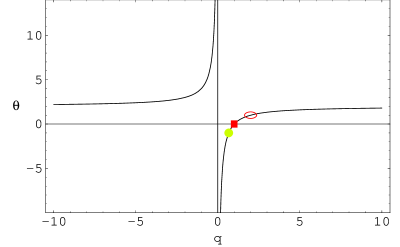
Figure 1: A graph for the parameter $\theta(q)$. Three models are located at GB($\theta(2/3)=-1$), 4D($\theta(1)=0$), and RS-II($\theta(2)=1$), respectively.

In the Gauss-Bonnet high-energy regime of $\sigma/\sigma_{0}\gg 1$ with the matter energy density $\sigma=\rho+\lambda$ and $1/\sigma_{0}=\sqrt{\alpha/2}\kappa^{2}_{5}$, we have a non-standard cosmology called “GB” model. When the energy density is far below the 5D/string scale ($\lambda/\sigma_{0}\ll\sigma/\sigma_{0}\ll 1$) but $\rho\gg\lambda$, we have the brane cosmology in high-energy regime called as “RS-II” model. The four-dimensional cosmology(“4D”) is recovered when $\rho/\sigma_{0}\ll\sigma/\sigma_{0}\ll 1$ but with $\rho\ll\lambda$. A plot for $\theta(q)$ is shown in Fig.1. We wish to comment on the two limiting cases of $q\to 0$ and $q\to\infty$. In the case of $q\to 0~{}(\theta\to\infty)$, one recovers de Sitter spacetime when $\beta^{2}_{0}\propto\Lambda$, whereas in the case of $q\to\infty~{}(\theta=2)$, one finds an interesting case in the power-law inflation.

Introducing an inflaton $\phi$ confined to the brane, one finds the equation

$$\ddot{\phi}+3H\dot{\phi}=-V^{\prime},$$ (2)

where dot and prime denote the derivative with respect to time and $\phi$, respectively. Its energy density and pressure are given by $\rho=\dot{\phi}/2+V$ and $p=\dot{\phi}/2-V$. From now on we use the slow-roll formalism for inflation: an accelerated universe $(\ddot{a}>0)$ is driven by a single scalar field slowly rolling down its potential toward a local minimum. This means that Eqs.(1) and (2) take the following form approximately:

$$H^{2}\approx\beta^{2}_{q}V^{q},~{}\dot{\phi}\approx-V^{\prime}/3H.$$ (3)

In order to take this approximation into account, we introduce Hubble slow-roll parameters (called H-SR towers) on the brane as

$$\epsilon_{1}\equiv-\frac{\dot{H}}{H^{2}}\approx\frac{3q\beta^{2-\theta}_{q}}{2}\frac{\dot{\phi}^{2}}{H^{2-\theta}},~{}~{}\delta_{n}\equiv\frac{1}{H^{n}\dot{\phi}}\frac{d^{n+1}\phi}{dt^{n+1}}$$ (4)

which satisfy the slow-roll condition: $\epsilon_{1}<\xi,~{}|\delta_{n}|<\xi^{n}$ for some small perturbation parameter $\xi$ defined on the brane. Here the subscript denotes slow-roll (SR)-order in the slow-roll expansion. We note that the original definition of H-SR parameters is independent of $q$ because these are constructed in a geometric way.

3 Cosmological parameter calculation

We are now in a position to calculate cosmological parameters using the Mukhanov’s formalism for scalar perturbations. We introduce a new variable $u^{q}\equiv aQ^{q}=a(\delta\phi^{q}-\dot{\phi}\psi/H)$ where $\delta\phi^{q}$ is a perturbed inflaton. $\psi$ is a perturbed metric function defined in $ds^{2}=-(1+2A)dt^{2}+(1+2\psi)a^{2}d{\bf x}\cdot d{\bf x}$. Its Fourier modes $u^{q}_{k}$ in the linear perturbation theory satisfies the Mukhanov equation:

$$\frac{d^{2}u^{q}_{k}}{d\tau^{2}}+\left(k^{2}-\frac{1}{z}\frac{d^{2}z}{d\tau^{2}}\right)u^{q}_{k}=0,$$ (5)

where the $q$-dependent potential-like term is given by

$$\frac{1}{z}\frac{d^{2}z}{d\tau^{2}}=2a^{2}H^{2}\Big{(}1+\epsilon_{1}+\frac{3}{2}\delta_{1}+\frac{1}{q}\epsilon_{1}^{2}+2\epsilon_{1}\delta_{1}+\frac{1}{2}\delta_{2}\Big{)}.$$ (6)

Here $\tau$ is the conformal time defined by $d\tau=dt/a$, and $z=a\dot{\phi}/H$ encodes all information about a slow-roll inflation with $\dot{\phi}=\sqrt{\rho+p}$.

Before we proceed, we have to mention that Eq.(5) is the nearly same form as in the conventional 4D perturbation theory[30, 31, 32]. It is well known that the perturbation theory of braneworlds including Randall-Sundrum and Gauss-Bonnet models is very different from the 4D perturbation theory[9, 10, 11, 12, 18, 19, 20, 23, 33]. Making use of the 4D Mukhanov equation to study the braneworld perturbation, the problem is that this equation incorporates 4D metric (scalar) perturbations only and thus there is no justification for using this to describe the effect of 5D gravity on the brane. This falls short of being a full 5D calculation as is required by the braneworld scenario. The 5D metric perturbations entered at first order and second order corrections to the perturbed equation[25]. Therefore it is not evident that the Mukhanov equation is reliable for studying the 5D brane cosmology. However, it was shown recently that even though the effect of 5D metric perturbations on inflation appears to be large on small-scales (sub-horizon), on large-scales (super-horizon) this effect is smaller certainly than first order corrections to de Sitter background[26]. Further, the effect of 5D metric perturbations is very small, at low energies, on super-horizon and also this is suppressed, even at high energies, on super-horizon. In Appendix A, we derive the Mukhanov equation including 5D metric perturbations from Koyama and Soda expression (Eq.(C.5) in Ref.[25]). Therefore it is sensible to use the Mukhanov equation (5) to compute first order corrections to cosmological parameters on the super-horizon scale.

In general its asymptotic solutions are obtained as

$$u^{q}_{k}\longrightarrow\left\{\begin{array}[]{l l l}\frac{1}{\sqrt{2k}}e^{-ik\tau}&\mbox{as}&-k\tau\rightarrow\infty\\ {\cal C}^{q}_{k}z&\mbox{as}&-k\tau\rightarrow 0.\end{array}\right.$$ (7)

The first solution corresponds to a plane wave on scale much smaller than the Hubble horizon of $d_{H}=1/H$ (sub-horizon regime), while the second is a growing mode on scale much larger than the Hubble horizon (super-horizon regime). Using a relation of $R^{q}_{c{\bf k}}=-u^{q}_{\bf k}/z$ with $u^{q}_{\bf k}(\tau)=a_{\bf k}u^{q}_{k}(\tau)+a^{\dagger}_{-{\bf k}}u^{q*}_{k}(\tau)$ and a definition of $P^{q}_{R_{c}}(k)\delta^{(3)}({\bf k}-{\bf l})=\frac{k^{3}}{2\pi^{2}}<R^{q}_{c{\bf k}}(\tau)R^{q\dagger}_{c{\bf l}}(\tau)>$, one finds the power spectrum for a curvature perturbation in the super-horizon regime

$$P^{q}_{R_{c}}(k)=\left(\frac{k^{3}}{2\pi^{2}}\right)\lim_{-k\tau\rightarrow 0}\left|\frac{u^{q}_{k}}{z}\right|^{2}=\frac{k^{3}}{2\pi^{2}}|{\cal C}^{q}_{k}|^{2}.$$ (8)

Our task is to find ${\cal C}^{q}_{k}$ by solving the Mukhanov equation (5). In general it is hard to solve this equation. However, we can solve it using either the slow-roll approximation [13] or the slow-roll expansion[16]. In the slow-roll approximation we take $\epsilon_{1}$ and $\delta_{1}$ to be constant. Thus this method could not be considered as a general approach beyond the first-order correction to the power spectrum[34, 35]. In order to show different power spectra depending on $q$, one uses the slow-roll expansion based on Green’s function technique. A step to consider is a slowly varying nature of slow-roll parameters implied by $\dot{H}=-\frac{3}{2}q\beta^{2}_{q}\rho^{q-1}(\dot{\phi})^{2}$ and $\ddot{H}=2H\dot{H}[-(1-1/q)\epsilon_{1}+\delta_{1}]$:

$$\dot{\epsilon}_{1} = 2H\Big{(}\epsilon_{1}^{2}/q+\epsilon_{1}\delta_{1}\Big{)},~{}\dot{\delta}_{1}=H(\epsilon_{1}\delta_{1}-\delta^{2}_{1}+\delta_{2}),$$ (9)

$$\dot{\delta_{2}} = H(2\epsilon_{1}\delta_{2}-\delta_{1}\delta_{2}+\delta_{3}),~{}\dot{\delta_{3}}=H(3\epsilon_{1}\delta_{3}-\delta_{1}\delta_{3}+\delta_{4})$$ (10)

which means that derivative of slow-roll parameters with respect to time increases their SR order by one in the slow-roll expansion. Note that except $\dot{\epsilon_{1}}$, all of $\dot{\delta}_{n}$ are independent of $q$. In this sense our choice for H-SR towers is convenient to investigate patch cosmology in compared with others in Ref.[14, 15]. After a lengthly calculation following ref.[16], we find the $q$-power spectrum

$$P^{q}_{R_{c}}(k) = \frac{H^{4}}{(2\pi)^{2}\dot{\phi}^{2}}\left\{1-2\epsilon_{1}+2\alpha(2\epsilon_{1}+\delta_{1})\right.$$

$$\left.+\left((8-4/q)\alpha^{2}-4(1-1/q)\alpha-(19+4/q)+(2+1/3q)\pi^{2}\right)\epsilon_{1}^{2}\right.$$

$$\left.+\left(3\alpha^{2}+2\alpha-22+29\pi^{2}/12\right)\epsilon_{1}\delta_{1}+\left(3\alpha^{2}-4+5\pi^{2}/12\right)\delta_{1}^{2}+\left(-\alpha^{2}+\pi^{2}/12\right)\delta_{2}\right\}$$

and the right hand side should be evaluated at horizon crossing of $k=aH$. $\alpha$ is defined by $\alpha=2-\ln 2-\gamma\simeq 0.7296$ where $\gamma$ is the Euler-Mascheroni constant, $\gamma\simeq 0.5772.$ We note that $q-$dependent terms appear only in coefficient of $\epsilon_{1}^{2}$. Using $\frac{d\epsilon_{1}}{d\ln k}=2(\epsilon_{1}^{2}/q+\epsilon_{1}\delta_{1})/(1-\epsilon_{1}),~{}\frac{d\delta_{1}}{d\ln k}=(\epsilon_{1}\delta_{1}-\delta_{1}^{2}+\delta_{2})/(1-\epsilon_{1}),~{}\frac{d\delta_{2}}{d\ln k}=(2\epsilon_{1}\delta_{2}-\delta_{1}\delta_{2}+\delta_{3})/(1-\epsilon_{1})$, and $\frac{d\delta_{3}}{d\ln k}=(3\epsilon_{1}\delta_{3}-\delta_{1}\delta_{3}+\delta_{4})/(1-\epsilon_{1})$, the $q$-spectral index defined by

$$n_{s}^{q}(k)=1+\frac{d\ln P^{q}_{R_{c}}}{d\ln k}$$ (12)

can be calculated up third order

$$n^{q}_{s}(k)= 1-4\epsilon_{1}-2\delta_{1}+(-4-4/q+8\alpha/q)\epsilon_{1}^{2}+(10\alpha-6)\epsilon_{1}\delta_{1}-2\alpha\delta_{1}^{2}+2\alpha\delta_{2}$$

$$+\left(-16\alpha^{2}/q^{2}+(16/q^{2}+24/q)\alpha-4-16/q^{2}-88/q+(4/3q^{2}+8/q)\pi^{2}\right)\epsilon_{1}^{3}$$

$$+\left(-(26/q+5)\alpha^{2}+(32+28/q)\alpha-112-60/q+(125/12+37/6q)\pi^{2}\right)\epsilon_{1}^{2}\delta_{1}$$

$$+\left(-3\alpha^{2}+4\alpha-30+13\pi^{2}/4\right)\epsilon_{1}\delta_{1}^{2}+\left(-7\alpha^{2}+8\alpha-22+31\pi^{2}/12\right)\epsilon_{1}\delta_{2}$$

$$+\left(-2\alpha^{2}+8-5\pi^{2}/6\right)\delta_{1}^{3}+\left(3\alpha^{2}-8+3\pi^{2}/4\right)\delta_{1}\delta_{2}+\left(-\alpha^{2}+\pi^{2}/12\right)\delta_{3}.$$

Here we find three changes in $\epsilon_{1}^{2},~{}\epsilon^{3}_{1}$ and $\epsilon^{2}_{1}\delta_{1}$. Finally the $q$-running spectral index up to fourth order is determined by

$$\frac{d}{d\ln k}n^{q}_{s} = -8\epsilon^{2}_{1}/q-10\epsilon_{1}\delta_{1}+2\delta^{2}_{1}-2\delta_{2}$$

$$+ \left(-16/q^{2}-24/q+32\alpha/q^{2}\right)\epsilon^{3}_{1}$$

$$+ \left(-32-28/q+(10+52/q)\alpha\right)\epsilon^{2}_{1}\delta_{1}$$

$$+ (6\alpha-4)\epsilon_{1}\delta^{2}_{1}+(14\alpha-8)\epsilon_{1}\delta_{2}+4\alpha\delta^{3}_{1}-6\alpha\delta_{1}\delta_{2}+2\alpha\delta_{3}$$

$$+ \left(-96\alpha^{2}/q^{2}+(96/q^{3}+176/q^{2})\alpha-(96/q^{3}+544/q^{2}+48/q)+(8/q^{3}+48/q^{2})\pi^{2}\right)\epsilon_{1}^{4}$$

$$+ \left(-(200/q^{2}+46/q+5)\alpha^{2}+(208/q^{2}+352/q+42)\alpha\right)\epsilon_{1}^{3}\delta_{1}$$

$$+ \left(-(336/q^{2}+1064/q+168)+(98/3q^{2}+575/6q+125/12)\pi^{2}\right)\epsilon_{1}^{3}\delta_{1}$$

$$+ \left(-(84/q+21)\alpha^{2}+(92/q+100)\alpha-(240/q+400)+(25/q+151/4)\pi^{2}\right)\epsilon_{1}^{2}\delta_{1}^{2}$$

$$+ \left(-(40/q+19)\alpha^{2}+(44/q+62)\alpha-(104/q+164)+(34/3q+187/12)\pi^{2}\right)\epsilon_{1}^{2}\delta_{2}$$

$$+ \left(-6\alpha^{2}+4\alpha+24-5\pi^{2}/2\right)\epsilon_{1}\delta_{1}^{3}+\left(-4\alpha^{2}+10\alpha-106+34\pi^{2}/3\right)\epsilon_{1}\delta_{1}\delta_{2}$$

$$+ \left(-10\alpha^{2}+10\alpha-22+17\pi^{2}/6\right)\epsilon_{1}\delta_{3}+\left(6\alpha^{2}-24+5\pi^{2}/2\right)\delta_{1}^{4}$$

$$+ \left(-12\alpha^{2}+40-4\pi^{2}\right)\delta_{1}^{2}\delta_{2}+\left(4\alpha^{2}-8+2\pi^{2}/3\right)\delta_{1}\delta_{3}$$

$$+ \left(3\alpha^{2}-8+3\pi^{2}/4\right)\delta_{2}^{2}+\left(-\alpha^{2}+\pi^{2}/12\right)\delta_{4}.$$

Here we have several changes in $\epsilon_{1}^{2},~{}\epsilon_{1}^{3},~{}\epsilon_{1}^{2}\delta_{1},~{}\epsilon_{1}^{4},~{}\epsilon_{1}^{3}\delta_{1},~{}\epsilon_{1}^{2}\delta_{1}^{2},~{}\epsilon_{1}^{2}\delta_{2}$. Up to now we calculate the power spectrum, spectral index, and running spectral index for slow-roll inflations in patch cosmology. If one uses the slow-roll approximation, there is no apparent distinction in power spectrum between GB, 4D, and RS-II. However, as are shown in Eqs.(3), (3), and (3), several modifications appear in the higher-order corrections. This is our motivation of why to calculate up to higher-order corrections using the slow-roll expansion. That is, we need to know the apparent distinction between GB, 4D, and RS-II (three models of patch cosmology) when applying them to describe the inflationary perturbations.

We note here that first order calculations in Eq.(3), second order calculations in Eq.(3), and third order calculations in Eq.(3) are only reliable if one takes into 5D metric perturbations account seriouly.

4 Power-law inflation

As a concrete example, we choose the power-law inflation like $a(t)\sim t^{p}$ to test patch cosmology. Although second order corrections are very small in the slow-roll limit and their reliability is not guaranteed, we calculate cosmological parameters up to second order to understand a degeneracy between the standard and brane inflations. Then Hubble slow-roll parameters (H-SR) are determined by

$$\epsilon_{1}=\frac{1}{p},~{}\delta_{1}=-\frac{1}{pq},~{}\delta_{2}=\frac{1+q}{(pq)^{2}},~{}\delta_{3}=-\frac{2q^{2}+3q+1}{(pq)^{3}},~{}\delta_{4}=\frac{6q^{3}+11q^{2}+6q+1}{(pq)^{4}}$$ (15)

which are obtained from relations in Eq. (9) after setting $\epsilon_{1}=1/p$[11]. This inflation goes very well with the slow-roll expansion. All of H-SR towers are constant for power-law inflations. The $q$-power spectrum takes the form

$$P^{PI,q}_{R_{c}}(k) = \frac{H^{4}}{(2\pi)^{2}\dot{\phi}^{2}}\Big{[}1+\frac{1}{p}\Big{(}4\alpha-\frac{2\alpha}{q}-2\Big{)}$$

$$+ \frac{1}{p^{2}}\Big{\{}(\frac{2}{q^{2}}-\frac{8}{q}+8)\alpha^{2}-(\frac{2}{q}-4)\alpha+\frac{-8+\pi^{2}}{2q^{2}}+\frac{18-2\pi^{2}}{q}-19+2\pi^{2}\Big{\}}\Big{]}$$

$$= \frac{H^{4}}{(2\pi)^{2}\dot{\phi}^{2}}\Big{[}1+\frac{1}{p}\Big{(}-\frac{1.4592}{q}+0.9184\Big{)}+\frac{1}{p^{2}}\Big{(}\frac{1.99943}{q^{2}}-\frac{4.53858}{q}+2.07934\Big{)}\Big{]}.$$

The $q$-spectral index can be easily calculated up to third order

$$n^{PI,q}_{s}(k)=1-4\Big{(}\frac{1}{p}+\frac{1}{p^{2}}+\frac{1}{p^{3}}\Big{)}\Big{(}1-\frac{1}{2q}\Big{)}.$$ (17)

Finally, the $q$-running spectral index is found to be zero up to $1/p^{4}$,

$$\frac{dn^{PI,q}_{s}}{d\ln k}=0.$$ (18)

Even though the running spectral index has a complicated from, we find that for power-law inflations, $\frac{dn^{q}_{s}}{d\ln k}=0$, irrespective of $q$. In the case of together $q\to 0$ with $p\to\infty$ but $pq\to$ a finite quantity (equivalently, $\epsilon_{1},~{}\delta_{n}\to 0$), one finds de Sitter inflation with $n_{s}^{PI,q\to 0}=1$. This corresponds to the extreme slow-roll regime (ESR) with $V$=nearly constant.

On the other hand, in order to obtain potential slow-roll parameters (V-SR), we have to choose explicit potentials which give rise to power-law inflations (see Appendix B). These are given by[15]

$$V^{GB}\sim\phi^{6},~{}~{}V^{4D}\sim e^{-\sqrt{2/p}~{}\phi},~{}~{}V^{RS-II}\sim\phi^{-2}.$$ (19)

Table 1: Power-law inflation potentials and potential slow-roll parameters (V-SR) in patch cosmology.

model	potential	V-SR
GB	$V^{GB}=\frac{1}{128}\Big{(}\frac{\kappa^{2}_{5}}{16\alpha}\Big{)}^{2}\frac{2p-1}{p^{4}}\phi^{6}$	$\epsilon^{V}_{1}=[(2p-1)/2p^{4}]^{1/3},~{}\delta^{V}_{1}=-(3/2)[(2p-1)/2p^{4}]^{1/3},~{}\delta^{V}_{2}=(15/4)[(2p-1)/2p^{4}]^{2/3},~{}\delta^{V}_{3}=-(105/8)[(2p-1)/2p^{4}],~{}\delta^{V}_{4}=(945/16)[(2p-1)/2p^{4}]^{4/3}$
4D	$V^{4D}=V_{0}\exp(-\sqrt{2\kappa^{2}_{4}/p}~{}\phi)$	$\epsilon^{V}_{1}=1/p,~{}\delta^{V}_{1}=-1/p,~{}\delta^{V}_{2}=2/p^{2},~{}\delta^{V}_{3}=-6/p^{3},~{}\delta^{V}_{4}=24/p^{4}$
RS-II	$V^{RS}(\phi)=\frac{4(6p-1)}{3}\frac{\lambda}{\kappa^{2}_{4}}\frac{1}{\phi^{2}}$	$\epsilon^{V}_{1}=6/(6p-1),~{}\delta^{V}_{1}=-3/(6p-1),~{}\delta_{2}^{V}=27/(6p-1)^{2},~{}\delta_{3}^{V}=-405/(6p-1)^{3},~{}\delta_{4}^{V}=8505/(6p-1)^{4}$

Instead of an exponential potential $V^{4D}$ for the standard inflation, a monomial potential of $V^{GB}$ and an inverse power-law potential of $V^{RS}$ are suitable for power-law inflation. Choosing coefficients in potentials appropriately, all will take similar shapes during inflation. Their potentials and corresponding slow-roll parameters appear in TABLE I. For a large $p>1$, $\epsilon_{1}\simeq\epsilon_{1}^{V},~{}\delta_{n}\simeq\delta_{n}^{V}$ are found for GB and RS-II cases, whereas one obtains the exact relations of $\epsilon_{1}=\epsilon_{1}^{V},~{}\delta_{n}=\delta_{n}^{V}$ for 4D case.

According to WMAP data[4, 5, 6], power spectrum normalization at $k_{0}=0.05{\rm Mpc}^{-1}$ is given by ${\cal A}=0.833^{+0.086}_{-0.083}$ where a normalization factor ${\cal A}$ is defined by $P^{ESR}_{R_{c}}=\frac{H^{4}}{(2\pi)^{2}\dot{\phi}^{2}}\times{\cal A}=2.95\times 10^{-9}\times{\cal A}$ and scalar spectral index is $n_{s}=0.93^{+0.03}_{-0.03}$ at $k_{0}=0.05{\rm Mpc}^{-1}$. Running spectral index is $dn_{s}/d\ln{k}=-0.031^{+0.016}_{-0.018}$ at $k_{0}=0.05{\rm Mpc}^{-1}$ and tensor-to-scalar ratio at $k_{0}=0.002{\rm Mpc}^{-1}$ is $R<0.90$ (95%CL).

As is shown in TABLE II, there exist slightly small changes in cosmological parameters. Different potentials give slightly different power spectra and spectral indices but give the same running spectral index. Apparently we find blue (red) power spectrum corrections to RS-II (GB,4D) inflations (see Fig. 2). We note that this is not a crucial result because we measure only a normalization factor ${\cal A}$ of the power spectrum from the WMAP. Also we have red spectral indices for all cases (see Fig. 3).

Table 2: Power spectrum normalization $\Big{(}{\cal A}^{PI}\Big{)}$, spectral index $\Big{(}n_{s}^{PI}\Big{)}$, and running spectral index $\Big{(}\frac{dn^{PI}_{s}}{d\ln k}\Big{)}$ based on H-SR towers. ^a Here $\approx 0$ means $-7.10543\times 10^{-15}/p^{3}+8.52651\times 10^{-14}/p^{4}\approx 0$.

model	${\cal A}^{PI}$	$n_{s}^{PI}$	$\frac{dn^{PI}_{s}}{d\ln k}$
GB	$1-\frac{1.2740}{p}-\frac{0.229741}{p^{2}}$	$1-\frac{1}{p}-\frac{1}{p^{2}}-\frac{1}{p^{3}}$	$\approx 0~{}^{\rm a}$
4D	$1-\frac{0.540726}{p}-\frac{0.459731}{p^{2}}$	$1-\frac{2}{p}-\frac{2}{p^{2}}-\frac{2}{p^{3}}$	0
RS-II	$1+\frac{0.1888}{p}+\frac{0.309928}{p^{2}}$	$1-\frac{3}{p}-\frac{3}{p^{2}}-\frac{3}{p^{3}}$	0

As a guideline to the power-law inflation, choosing $p=101$ leads to ${\cal A}^{PI,RS-II}=1,~{}1.00187,~{}1.0019$ for zero, first, second order corrections, respectively, whereas ${\cal A}^{PI,4D}=1,~{}0.994646,~{}0.99461$ and ${\cal A}^{PI,GB}=1,~{}0.987386(0.987407),~{}0.987364(0.987385)$. Also we find that $n_{s}^{PI,RS-II}=0.970297(0.970248),~{}0.970003(0.969953),~{}0.97(0.96995)$ for zero, first, second-order corrections, while $n_{s}^{PI,4D}=0.980198,~{}0.980002,~{}0.98$ and $n_{s}^{PI,GB}=0.990099(0.990115),~{}0.990001(0.990018),~{}0.99(0.990017)$. Here ($\cdots$) are calculated using V-SR towers (see TABLE III). In the case of $q\to\infty$, we have ${\cal A}^{PI,\infty}=1,~{}1.00909,~{}1.0093$ and $n_{s}^{PI,\infty}=0.960396,~{}0.960004,~{}0.96$. Although its potential is not yet known, this case provides us the smallest spectral index and the largest power spectrum. We find from the above that first and second-order corrections lie within the uncertainty. Fitting of $n_{s}$ to the WMAP seems to be beyond the uncertainty for a $p=101$ case. According to Ref.[36], however, a constraint on 4D power-law inflation is given by $0<\epsilon_{1}<0.019$ and $p>53$. Here we choose an appropriate $p$ between $50<p<110$ to fit the data within the uncertainty. In the case of GB power-law inflation, we may loosen the lower bound of $p$ to fit the data.

Since recent observations including WMAP have restricted viable inflation models to regions close to the slow-roll limit, our second-order corrections to the patch cosmology are rather small. If one uses V-SR towers with $50<p<110(2p-1\simeq 2p,~{}6p-1\simeq 6p)$, also we lead to the same conclusion (see TABLE III). Hence we confirm that in the slow-roll limit, observations of the primordial perturbation spectra cannot distinguish between GB, RS-II, and 4D power-law inflations[10]. Hence we need to introduce the tensor spectrum, especially for the tensor-to-scalar ratio.

Table 3: Power spectrum, spectral index, and running spectral index based on V-SR towers. ^b Here $\approx 0$ means $-7.10543\times 10^{-15}\Big{[}(2p-1)/(2p^{4})\Big{]}+8.52651\times 10^{-14}\Big{[}(2p-1)/(2p^{4})\Big{]}^{4/3}\approx 0$.

model	${\cal A}^{PI}$	$n_{s}^{PI}$	$\frac{dn^{PI}_{s}}{d\ln k}$
GB	$1-1.2740\Big{[}\frac{2p-1}{2p^{4}}\Big{]}^{\frac{1}{3}}-0.229741\Big{[}\frac{2p-1}{2p^{4}}\Big{]}^{\frac{2}{3}}$	$1-\Big{[}\frac{2p-1}{2p^{4}}\Big{]}^{\frac{1}{3}}-\Big{[}\frac{2p-1}{2p^{4}}\Big{]}^{\frac{2}{3}}-\Big{[}\frac{2p-1}{2p^{4}}\Big{]}$	$\approx 0~{}^{\rm b}$
4D	$1-\frac{0.540726}{p}-\frac{0.459731}{p^{2}}$	$1-\frac{2}{p}-\frac{2}{p^{2}}-\frac{2}{p^{3}}$	0
RS-II	$1+0.1888\Big{[}\frac{6}{6p-1}\Big{]}+0.309928\Big{[}\frac{6}{6p-1}\Big{]}^{2}$	$1-3\Big{[}\frac{6}{6p-1}\Big{]}-3\Big{[}\frac{6}{6p-1}\Big{]}^{2}-3\Big{[}\frac{6}{6p-1}\Big{]}^{3}$	0

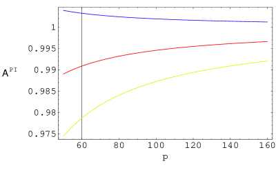
Figure 2: Plot of the power spectrum normalization ${\cal A}^{PI}$ for power-law inflation with $a(t)\sim t^{p}$. From the top curve to the bottom one, one finds RS-II(blue), 4D(red), and GB(yellow), respectively. An appropriate value $p$ is between $p=50$ and $p=110$, and a line of $p=60$ is introduced for comparison.

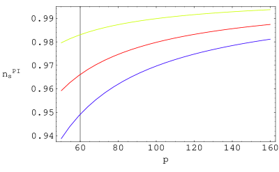
Figure 3: Plot of the spectral index $n_{s}^{PI}$ for power-law inflation with $a(t)\sim t^{p}$. From the top curve to the bottom one, one finds GB(yellow), 4D(red), and RS-II(blue), respectively. An appropriate value $p$ is between $p=50$ and $p=110$, and a line of $p=60$ is introduced for comparison.

5 Consistency relation in patch cosmology

The tensor-to-scalar ratio $R$ is defined by

$$R=16\frac{A_{T,q}^{2}}{A_{S,q}^{2}}.$$ (20)

Here the $q$-scalar amplitude to zero order is given by

$$A_{S,q}^{2}=\frac{4}{25}P_{R_{c}}^{q,ESR}$$ (21)

with the extreme slow-roll power spectrum

$$P_{R_{c}}^{q,ESR}=\frac{3q\beta^{2-\theta}_{q}}{(2\pi)^{2}}\frac{H^{2+\theta}}{2\epsilon_{1}}=\frac{1}{(2\pi)^{2}}\frac{H^{4}}{\dot{\phi}^{2}}.$$ (22)

The 4D($q=1$) tensor amplitude to zero order is given by

$$A_{T,4D}^{2}=\frac{1}{50}P_{T}^{ESR}$$ (23)

with $P_{T}^{ESR}=(2\kappa_{4})^{2}\Big{(}\frac{H}{2\pi}\Big{)}^{2}$ because a tensor can be expressed in terms of two scalars like $\delta\phi$ with a factor $2\kappa_{4}$. On the other hand, the tensor spectra for GB($q=2/3$) and RS-II($q=2$) are known only for de Sitter brane[33, 23]. These are given by

$$A_{T,q}^{2}=A_{T,4D}^{2}F_{\alpha}^{2}(H/\mu),$$ (24)

where

$$F_{\beta}^{-2}(x)=\sqrt{1+x^{2}}-\Big{(}\frac{1-\beta}{1+\beta}\Big{)}x^{2}\sinh^{-1}\Big{(}\frac{1}{x}\Big{)}.$$ (25)

In three regimes, we approximate $F_{\beta}^{2}$ as $F_{q}^{2}$: $F_{1}^{2}=1\approx F_{\beta}^{2}(H/\mu\ll 1)$ for 4D case; $F_{2}^{2}=3H/(2\mu)\approx F_{\beta=0}^{2}(H/\mu\gg 1)$ for RS-II case; $F_{2/3}^{2}=(1+\beta)/(2\beta)(\mu/H)\approx F_{\beta}^{2}(H/\mu\gg 1)$ for GB case. The tensor amplitude to zero order is given by

$$A_{T,q}^{2}=\frac{3q\beta^{2-\theta}_{q}}{(5\pi)^{2}}\frac{H^{2+\theta}}{2\zeta_{q}(h)}$$ (26)

with $\zeta_{1}(h)=\zeta_{2/3}(h)=1$ and $\zeta_{2}(h)=2/3$[37]. Then the tensor-to-scalar ratio is determined by

$$R_{q}=16\frac{A_{T,q}^{2}}{A_{S,q}^{2}}=16\frac{\epsilon_{1}}{\zeta_{q}(h)}.$$ (27)

Considering $n_{T,1}=-2\epsilon_{1},~{}n_{T,2/3}=-\epsilon$ and $n_{T,2}=-3\epsilon_{1}$, one finds that

$$R_{1}=-8n_{T,1}=16\epsilon_{1},~{}R_{2}=-8n_{T,2}=24\epsilon_{1},~{}R_{2/3}=-16n_{T,2/3}=16\epsilon_{1}.$$ (28)

The above shows that the RS-II consistency relation is the same for that of 4D case but the GB consistency relation is different from RS-II and 4D cases.

In the de Sitter brane approach with $a\sim e^{Ht}$, we have no non-zero H-SR towers. The zero-order scalar amplitude for GB braneworld is given by $A_{S,dS}^{2}=A_{S,4D}^{2}G_{\beta}^{2}(H/\mu)$ where $G_{\beta}^{2}(x)=\Big{[}\frac{3(1+\beta)x^{2}}{2\sqrt{1+x^{2}}(3-\beta+2\beta x^{2})+2(\beta-3)}\Big{]}^{3}$. In the 4D limit, we have $G_{\beta}^{2}(H/\mu\ll 1)\approx 1$. In the GB regime, $G_{\beta}^{2}(H/\mu\gg 1)\approx\frac{27}{64}\Big{(}\frac{1+\beta}{\beta}\Big{)}^{3}\frac{\mu^{3}}{H^{3}}$, while in the RS-II regime, $G_{\beta=0}^{2}(H/\mu\gg 1)\approx\frac{H}{2\mu}$. These lead to $A_{S,q}^{2}=\frac{3q\beta^{2-\theta}_{q}}{(5\pi)^{2}}\frac{H^{2+\theta}}{2\epsilon_{1}}$. In the extreme slow-roll regime of $\epsilon_{1},~{}\delta_{n}\to 0$, one finds the same amplitude of $\frac{1}{(2\pi)^{2}}\frac{H^{4}}{\dot{\phi}^{2}}$, as found in the de Sitter brane approach. However, the de Sitter picture is basically different from ours because we work with slow-roll approximation of $\epsilon_{1}<\xi,|\delta_{n}|<\xi^{n}$ for $\xi<1$, but not with a case with $\epsilon_{1},\delta_{n}\to 0$ for de Sitter brane[38]. In other words, we work with $\rho+p=\dot{\phi}^{2}$ but not a case :$\rho+p\to 0\Rightarrow V=$ constant as in de Sitter brane. In the de Sitter brane approach, we cannot make any slow-roll approximation because de Sitter space means that $H$= constant during inflation. In this sense the slow-roll approximation to GB braneworld based on de Sitter brane to obtain a tensor spectrum leads to an obscure computation.

6 Discussions

Our second-order corrections which appear even slightly different from those of the standard inflation, could not play a role in distinguishing between GB, RS-II, 4D slow-roll inflations. Thus it is necessary to introduce the tensor power spectrum to distinguish them. The reason is as follows. These models are based on the same perturbation scheme given by the Mukhanov equation (5) with slightly different potential-like terms: $\frac{1}{z}\frac{d^{2}z}{d\tau^{2}}$. This patch cosmology with an inflaton gives us similar results in the slow-roll expansion except a relation of $\dot{\epsilon}_{1}=2H(\epsilon_{1}^{2}/q+\epsilon_{1}\delta_{1})$ which affects second-order and more higher-orders only. For three different potentials, we find the nearly same power-law inflation. In the slow-roll limit, these give us the nearly same cosmological parameters. Since an introduction of a Gauss-Bonnet term in the braneworld could not distinguish between GB, 4D, and RS-II, we need to introduce the tensor spectrum. Thus the observation of gravitational waves may be helpful to select a desired inflation model.

Even though there exist a $q$-dependent term of $-8\epsilon_{1}^{2}/q$ in the lowest-order of the running spectral index, we find that $\frac{dn^{q}_{s}}{d\ln k}=0$, irrespective of $q$, when choosing power-law potentials. This shows the nature of power-law inflation in the patch cosmology. It compares with the WMAP data of $dn_{s}/d\ln{k}=-0.031^{+0.016}_{-0.018}$ at $k_{0}=0.05{\rm Mpc}^{-1}$.

We have a few of comments on other cases in patch cosmology. From Eq.(17), for $q\to\infty$, one finds an interesting case of $n_{s}^{PI,\infty}\to 1-4(1/p+1/p^{2})$. Also we find a scale-invariant spectral index of $n_{s}=1$ for $q=1/2$, irrespective of $p$. Although we don’t know the corresponding model explicitly, it will be located beyond the GB high-energy regime. In the case of $q>1/2$, we have a red spectral index, whereas for $q<1/2$, we have a blue index. In the limit of $q\to 0$, unfortunately one finds a largely blue spectral index of $n_{s}^{PI,q\to 0}>1$ which is ruled out from the data. Hence an appropriate region to a patch parameter $q$ is given by $1/2\leq q<\infty$ which provides a restriction : $1-4(1/p+1/p^{2})<n_{s}\leq 1$.

Finally, we emphasize that our calculation based on the Mukhanov equation is reliable up first order corrections. At this stage we don’t know whether or not the second order corrections are smaller than the effect of 5D metric perturbations. Even though we calculate cosmological parameters up to second order to understand the power-law nature of patch cosmology, second order corrections are less important because these are rather small than first order corrections in the slow-roll limit and these are not yet proved to be reliable.

Acknowledgements

We thank Hungsoo Kim, H. W. Lee and G. Calcagni for helpful discussions. K. Kim was in part supported by KOSEF, Astrophysical Research Center for the Structure and Evolution of the Cosmos. Y. Myung was supported by the Korea Research Foundation Grant (KRF-2005-013-C00018).

.

Appendix A: Derivation of the Mukhanov equation including 5D metric perturbations.

We start with Eq.(C.5) in Ref.[25] expressed in terms of $Q=\delta\phi-\dot{\phi}\psi/H$,

$$\ddot{Q}+3H\dot{Q}+\frac{k^{2}}{a^{2}}Q+\Big{[}\frac{\ddot{H}}{H}-2\frac{\dot{H}V^{\prime}}{H\dot{\phi}}-2\Big{(}\frac{\dot{H}}{H}\Big{)}^{2}+V^{\prime\prime}\Big{]}Q=J.$$ (29)

Here $J$ is the contribution from the 5D metric perturbations given by

$$J=\frac{\dot{\phi}}{H}\Big{[}\Big{(}\frac{2\ddot{H}}{\dot{H}}-\frac{\dot{H}}{H}\Big{)}\Delta v+\frac{k^{2}}{3a^{2}}A+\frac{k^{2}}{3a^{2}}\Big{(}1-\frac{\dot{H}}{\alpha^{2}_{1}}\Big{)}\psi$$

$$+\frac{k^{4}}{9a^{4}}\Big{(}2-\frac{\dot{H}}{\alpha^{2}_{1}}\Big{)}\int dmE(m,k)l^{2}Z_{0}(ml/a)e^{-i\omega T(t)}\Big{]},$$ (30)

where the detailed information on the unknown functions ($\Delta v,\alpha_{1}^{2},E(m,k),\cdots$) are given by Ref.[25]. We note that the above equation is derived by using the braneworld scenario without the Gauss-Bonnet term. In this work we are interested in its patch approximation. We wish to derive the corresponding Mukhanov equation including the effect of 5D metric perturbations. Using $Q^{q}=u^{q}/a$, Eq.(2) and its derivative, and Eq.(4), we obtain the following equation from Eq.(29) exactly:

$$\frac{d^{2}u^{q}_{k}}{d\tau^{2}}+\left(k^{2}-\frac{1}{z}\frac{d^{2}z}{d\tau^{2}}\right)u^{q}_{k}=a^{3}J^{q}$$ (31)

with the $q$-dependent potential $\frac{1}{z}\frac{d^{2}z}{d\tau^{2}}$ in Eq.(6) and patch approximation $J^{q}$ to $J$. In the limit of $J^{q}\to 0$, we recover the Mukhanov equation (5). Koyama and Soda showed implicitly that $J\to 0$ could be achieved on super-horizon scale[25]. According to Koyama et al[26], it turns out that $J^{q=1}$ at low-energy of $H/\mu\ll 1$ and $J^{q=2}$ at high-energy of $H/\mu\gg 1$ with $\beta=0$ are smaller than first order corrections to on super-horizon scale. Similarly, we expect that $J^{q=2/3}$ at high-energy of $H/\mu\gg 1$ with $\beta\not=0$ is smaller than first order corrections. At this stage, we don’t know whether or not $J^{q}$ is smaller than second order corrections. At first order of the slow-roll expansion, the ratio $J^{q=2}$ to first-order term takes the form of $J^{q=2}/\dot{H}Q\sim\frac{k^{4}}{(aH)^{4}}$ at high energies and thus it goes to zero on super-horizon scale of $k\ll aH$. On the other hand, the ratio $J^{q=2}$ to second-order term takes the form of $J^{q=2}H^{2}/\dot{H}^{2}Q\sim\frac{1}{\epsilon_{1}}\frac{k^{4}}{(aH)^{4}}$ at high energies. If $k$ is enough large than $aH$ on super-horizon scale, it seems that the second order calculation is reliable. However, this does not show that the effect of 5D metric perturbations is less definitely than second order corrections. On the other hand, the effect of 5D metric perturbations is less certainly than first order corrections.

Appendix B: Potential slow-roll parameters in the patch cosmology

The potential slow-roll parameters (V-SR) are given by

$$\epsilon^{V}_{1}=\frac{q}{6\beta^{2}_{q}}\frac{V^{\prime 2}}{V^{1+q}},~{}~{}\delta^{V}_{1}=-\frac{1}{3\beta^{2}_{q}}\Big{[}\frac{V^{\prime\prime}}{V^{q}}-\frac{V^{\prime 2}}{V^{1+q}}\Big{]},$$ (32)

$$\delta_{2}^{V}=(-\frac{1}{3\beta^{2}_{q}})^{2} \Big{[} \frac{V^{\prime\prime\prime}V^{\prime}}{V^{2q}}+\frac{V^{\prime\prime 2}}{V^{2q}}-\frac{5q}{2}\frac{V^{\prime\prime}V^{\prime 2}}{V^{2q+1}}+\frac{q}{2}(q+1)\frac{V^{\prime 4}}{V^{2q+2}}\Big{]},$$ (33)

$$\delta_{3}^{V}=(-\frac{1}{3\beta^{2}_{q}})^{3} \Big{[} \frac{V^{\prime\prime\prime\prime}V^{\prime 2}}{V^{3q}}-4q\frac{V^{\prime\prime\prime}V^{\prime 3}}{V^{3q+1}}+9q\frac{V^{\prime\prime 2}V^{\prime 2}}{V^{3q+1}}+5q(5q+1)\frac{V^{\prime\prime}V^{\prime 4}}{V^{3q+2}}$$

$$+ 4\frac{V^{\prime\prime\prime}V^{\prime\prime}V^{\prime}}{V^{3q}}+\frac{V^{\prime\prime 3}}{V^{3q}}-\frac{q}{2}(q+1)(\frac{3q}{2}+2)\frac{V^{\prime 6}}{V^{3q+3}}\Big{]},$$

$$\delta_{4}^{V}=(-\frac{1}{3\beta^{2}_{q}})^{4} \Big{[} \frac{V^{\prime\prime\prime\prime\prime}V^{\prime 3}}{V^{4q}}+7\frac{V^{\prime\prime\prime\prime}V^{\prime\prime}V^{\prime 2}}{V^{4q}}-6q\frac{V^{\prime\prime\prime\prime}V^{\prime 4}}{V^{4q+1}}-42q\frac{V^{\prime\prime\prime}V^{\prime\prime}V^{\prime 3}}{V^{4q+1}}$$

$$+ q(\frac{57q}{4}+9)\frac{V^{\prime\prime\prime}V^{\prime 5}}{V^{4q+2}}-29q\frac{V^{\prime\prime 3}V^{\prime 2}}{V^{4q+1}}+q(\frac{197q}{4}+34)\frac{V^{\prime\prime 2}V^{\prime 4}}{V^{4q+2}}$$

$$- q(\frac{71}{4}q^{2}+\frac{139}{4}q+17)\frac{V^{\prime\prime}V^{\prime 6}}{V^{4q+3}}+11\frac{V^{\prime\prime\prime}V^{\prime\prime 2}V^{\prime}}{V^{4q}}+\frac{V^{\prime\prime 4}}{V^{4q}}$$

$$+ 4\frac{V^{\prime\prime\prime 2}V^{\prime 2}}{V^{4q}}+\frac{q}{2}(q+1)(\frac{3q}{2}+2)(2q+3)\frac{V^{\prime 8}}{V^{4q+4}}\Big{]}.$$

Here the prime($\prime$) denotes the derivative with respect to $\phi$.

References

[1] L. Randall and R. Sundrum, Phys. Rev. Lett. 83,
4690 (1999) [hep-th/9906064] .
[2] P. Binetruy, C. Deffayet and D. Langlois,
Nucl. Phys. B565, 269 (2000) [hep-th/9905012].
[3] P. Binetruy, C. Deffayet, U. Ellwanger, and D. Langlois, Phys. Lett. B477,
285 (2000) [hep-th/9910219].
[4] H. V. Peiris, et al, Astrophys. J. Suppl. 148 (2003) 213
[astro-ph/0302225].
[5]
C. L. Bennett, et al, Astrophys. J. Suppl. 148 (2003)
1[astro-ph/0302207].
[6]
D. N. Spergel, et al, Astrophys. J. Suppl. 148 (2003)
175[astro-ph/0302209].
[7] P. Mukherjee and Y. Wang, Astrophys. J. 599 (2003) 1
[astro-ph/0303211].
[8]
S. L. Bridle, A. M. Lewis, J. Weller and G. Efstathiou, Mon. Not.
Roy. Astron. Soc. 342 (2003) L72[astro-ph/0302306].
[9] R. Maartens, D. Wands, B. A. Bassett, and I. P.
Heard, Phys. Rev. D62 (2000) 041301 [hep-ph/9912464].
[10] A. R. Liddle and A. N. Taylor, Phys. Rev. D 65 (2002)
041301 [astro-ph/0109412].
[11] E. Ramirez and A. R. Liddle,
asrtro-ph/0309608.
[12] S. Tsujikawa and A. R. Liddle,
JCAP 0403 (2004) 001 [asrtro-ph/0312162].
[13] E. D. Stewart and D. H. Lyth, Phys. Lett. B302 (1993) 171.
[14] D. J. Schwarz, C. A. Terrero-Escalante, and A. A.
Garcia, Phys.Lett. B 517 (2001) 243 [astro-ph/0106020].
[15] G. Calcagni, Phys. Rev. D 69 (2004) 103508
[hep-ph/0402126].
[16] E. Stewart and J.-O. Gong, Phys. Lett. B 510 (2001) 1
[astro-ph/0101225].
[17] Kyong Hee Kim, H. W. Lee, and Y. S. Myung,
Phys. Rev. D 70 (2004) 027302 [hep-th/0403210].
[18] G. Huey and J. E. Lidsey, Phys. Lett. B 514 (2001)
217 [astro-ph/0104006].
[19]
G. Huey and J. E. Lidsey, Phys. Rev. D 66 (2002) 043514
[astro-ph/0205236].
[20]
D. Seery and A. Taylor, astro-ph/0309512.
[21] G. Calcagni, hep-ph/0310304.
[22] G. Calcagni, JCAP 0406 (2004) 002 [hep-ph/0312246].
[23] J. F. Dufaux, J. E. Lidsey, Maartens, and M. Sami,
astro-ph/0404161.
[24] S. Tsujikawa, M. Sami, and R. Maartens, astro-ph/0406078.
[25] K. Koyama and J. Soda, Phys. Rev. D 65
(2002) 023514 [hep-th/0108003].
[26] K. Koyama, D. Langlios, R. Maartens, and D. Wands,
hep-th/0408222,
[27] Y. S. Myung and J. Y. Kim, Class. Quant. Grav. 20 (2003) L169
[hep-th/0304033].
[28]
R.-G. Cai, Y. S. Myung, and N. Ohta, Class. Quant. Grav. 18
(2001) 5429 [hep-th/0105070].
[29]
N. J. Kim, H. W. Lee, Y.S. Myung, and Gungwon Kang,
Phys. Rev. D 64 (2001) 064022
[hep-th/0104159].
[30] V. F. Mukhanov, JETP Lett. 41 (1985) 493.
[31] V. F. Mukhanov, Phys. Lett. B 218 (1989) 17.
[32] M. Sasaki, Prog. Theor. Phys. 76 (1986) 1036.
[33] D. Langlois, R. Maartens, and D. Wands, Phys. Lett. B 489 (2000)
259 [hep-th/0006007].
[34] Hungsoo Kim, G. S. Lee, and Y. S. Myung, Mod. Phys. Lett. A 20 (2005) 271
[hep-th/0402018].
[35] Hungsoo Kim, G. S. Lee, H. W. Lee, and Y. S. Myung,
Phys. Rev. D 70 (2004) 043521 [hep-th/0402198].
[36] S. M. Leach and A. R. Liddle, Phys. Rev. D 68
(2003) 123508 [astro-ph/0306305].
[37] G. Calcagni, hep-th/0406006.
[38] N. Arkami-Hamed, Paolo Creminelli, S. Mukohyama, and M
Zaldarriaga, JCAP 0404 (2004) 001[hep-th/0312100].