Effect of clustering on extragalactic source counts with low-resolution instruments

Abstract

In the presence of strong clustering, low-resolution surveys measure the summed contributions of groups of sources within the beam. The counts of bright intensity peaks are therefore shifted to higher flux levels compared to the counts of individual sources detected with high-resolution instruments. If the beam-width corresponds a sizable fraction of the clustering size, as in the case of Planck/HFI, one actually detects the fluxes of clumps of sources. We argue that the distribution of clump luminosities can be modelled in terms of the two- and three-point correlation functions, and apply our formalism to the Planck/HFI $850\,\mu$m surveys. The effect on counts is found to be large and sensitive also to the evolution of the three-point correlation function; in the extreme case that the latter function is redshift-independent, the source confusion due to clustering keeps being important above the canonical $5\sigma$ detection limit. Detailed simulations confirm the reliability of our approach. As the ratio of the beam-width to the clustering angular size decreases, the observed fluxes approach those of the brightest sources in the beam and the clump formalism no longer applies. However, simulations show that also in the case of the Herschel/SPIRE $500\,\mu$m survey the enhancement of the bright source counts due to clustering is important.

1 Introduction

It has long been known (Eddington 1913) that the counts (or flux estimates) of low signal-to-noise sources are biased high. Contributions to the noise arise both from the instrument and from source confusion. The latter, which may dominate already at relatively bright fluxes in the case of low-resolution surveys, comprises the effect of Poisson fluctuations and of source clustering. For angular scales where the correlation of source positions is significant, the ratio of clustering to Poisson fluctuations increases with angular scale (De Zotti et al. 1996), so that the confusion limit can be set by the effect of clustering. This is likely the case for some far-IR and for sub-mm surveys from space, due to the relatively small primary apertures and to the presence of strongly clustered populations (Scott & White 1999; Haiman & Knox 1999; Magliocchetti et al. 2001; Perrotta et al. 2003; Negrello et al. 2004).

While the effect of Poisson confusion on source counts has been extensively investigated both analytically (Scheuer 1957; Murdoch et al. 1973; Condon 1974; Hogg & Turner 1998) and through numerical simulations (Eales et al. 2000; Hogg 2001; Blain 2001), the effect of clustering received far less attention. The numerical simulations by Hughes & Gaztañaga (2000) focused on the sampling variance due to clustering. Algorithms successfully simulating the 2D distribution of clustered sources over sky patches as well as over the full sky have been presented by Argüeso et al. (2003) and González-Nuevo et al. (2004), who also discussed several applications. Some efforts have been made to quantify theoretically the effect of clustering on the confusion noise but not on the source counts (Toffolatti et al. 1998; Negrello et al. 2004; Takeuchi & Ishii 2004).

In this paper we will use the counts of neighbours formalism (Peebles 1980, hereafter P80) and numerical simulations to address the effects of clustering on source fluxes as measured by low-angular resolution surveys and, consequently, on source counts. The formalism is described in Section 2, the numerical simulations in Section 3, while in Section 4 we present applications to the 850$\,\mu$m survey with Planck/HFI and to the 500$\,\mu$m Herschel/SPIRE surveys. In Section 5 we summarize our main conclusions.

We adopt a flat cold dark matter (CDM) cosmology with $\Omega_{0,\Lambda}=0.7$ and $h=H_{0}/100\,\hbox{km}\,\hbox{s}^{-1}\,\hbox{Mpc}^{-1}=0.7$, consistent with the first-year WMAP results (Spergel et al. 2003).

2 Formalism

While in the case of a Poisson distribution a source is observed on top of a background of unresolved sources that may be either above or below the all-sky average, in the case of clustering sources are preferentially located in over-dense environments and one therefore measures the sum of all physically related sources in the resolution element of the survey (on top of Poisson fluctuations due to unrelated sources seen in projection).

If the beam-width corresponds to a substantial fraction of the clustering size, the observed flux is, generally, well above that of any individual source. Thus, to estimate the counts we cannot refer to the source luminosity function, but must define the distribution of luminosities, $L_{cl}(z)$, of source “clumps”, as a function of redshift $z$. It has long been known (Kofman et al. 1994; Taylor & Watts 2000; Kayo et al. 2001) that a log-normal function is remarkably successful in reproducing the statistics of the matter-density distribution found in a number of N-body simulations performed within the CDM framework, not only in weakly non-linear regimes, but also in more strongly non-linear regimes, up to density contrasts $\delta\approx 100$. Furthermore, it displays the correct asymptotic behaviour at very early times, when the density field evolves linearly and its distribution is still very close to the initial Gaussian one (Coles & Jones 1991).

If light is a (biased) tracer of mass, fluctuations in the luminosity density should obey the same statistics of the matter-density field; we therefore adopt a log-normal shape for the distribution of $L_{cl}$. Such a function is completely specified by its first (mean) and second (variance) moments, that can be evaluated by using the counts of neighbours formalism. The mean number of objects inside a volume $V$ centered on a given source, $\langle N\rangle_{p}$, is [see Eq. (36.23) of P80]:

$$\langle N\rangle_{p}=n\int_{V}[1+\xi(r)]dV\ ,$$ (1)

where $n$ is the mean volume density of the sources and $\xi$ is their two-point spatial correlation function. The excess of objects (with respect to a random distribution) around the central one is then given by the second term on the right-hand side of this equation. The variance around the mean value $\langle N\rangle_{p}$ can instead be written as [Eq. (36.26) of P80]:

$$\langle(N-\langle N\rangle_{p})^{2}\rangle_{p}=\langle N\rangle_{p}~{}+~{}~{}~{}~{}~{}~{}~{}~{}~{}~{}~{}~{}~{}~{}~{}~{}~{}~{}~{}~{}~{}~{}~{}~{}~{}~{}~{}~{}~{}~{}~{}~{}~{}~{}~{}$$

$$~{}~{}~{}~{}n^{2}\int_{V}\int_{V}[\zeta(r_{1},r_{2})+\xi(r_{12})-\xi(r_{1})\xi(r_{2})]dV_{1}dV_{2}\ .$$ (2)

If the first term on the right-hand side dominates, the variance is approximately equal to the mean, as in the case of a Poisson distribution.

The second term on the right-hand side of Eq. (2) is related to the skewness of the source distribution and exhibits a dependence also on the reduced part of the three-point angular correlation function, $\zeta$, for which we adopt the standard hierarchical formula:

$$\zeta(r_{1},r_{2})=Q[\xi(r_{1})\xi(r_{2})+\xi(r_{1})\xi(r_{12})+\xi(r_{12})\xi(r_{2})].$$ (3)

In the local Universe, observational estimates of the amplitude $Q$ indicate nearly constant values, in the range $Q\simeq 0.6$–1.3, on scales smaller than $\sim$ 10 Mpc/h (Peebles & Groth 1975; Fry & Seldner 1982; Jing & Boerner 1998, 2004). On larger scales, i.e. in the weakly non-linear regime where $\xi\mathrel{\hbox to0.0pt{\raise-1.29167pt\hbox{${\scriptstyle\sim}$}\hss}\raise 2.58334pt\hbox{${\scriptstyle<}$}}1$, the non-linear perturbation theory - corroborated by N-body simulations - instead predicts $Q$ to show a dependence on the scale (Fry 1984; Fry et al. 1993; Jing & Boerner 1997; Gaztañaga & Bernardeau 1998; Scoccimarro et al. 1998).

From Eqs. (1) and (2) we can derive, at a given redshift $z$, the mean luminosity of the clump, $\overline{L}_{cl}$, and its variance, $\sigma^{2}_{L_{cl}}$:

$$\overline{L}_{cl}(z) = \overline{L}(z)$$ (4)

$$+ \int_{\cal{L}}dL^{\prime}K(z)L^{\prime}\Phi(L^{\prime},z)\cdot\int_{V}[1+\xi(r,z)]dV\$$

and

$$\!\!\!\!\!\!\!\!\!\!\sigma^{2}_{L_{cl}}(z)=\sigma^{2}_{L}+\int_{\cal{L}}dL^{\prime}K(z)L^{\prime 2}\Phi(L^{\prime},z)\int_{V}[1+\xi(r,z)]dV$$

$$~{}+~{}\left[\int_{\cal{L}}dL^{\prime}K(z)L^{\prime}\Phi(L^{\prime},z)\right]^{2}\cdot$$

$$\!\!\!\!\!\!\!\!\!\!\!\!\int_{V}\int_{V}[\zeta(r_{1},r_{2},z)+\xi(r_{12},z)-\xi(r_{1},z)\xi(r_{2},z)]dV_{1}dV_{2}.$$ (5)

In Eq. (4) $\overline{L}(z)$ represents the mean luminosity of the sources located at redshift $z$

$$\overline{L}(z)=\frac{\int_{\cal{L}}dL^{\prime}K(z)L^{\prime}\Phi(L^{\prime},z)}{\int_{\cal{L}}dL^{\prime}K(z)\Phi(L^{\prime},z)}$$ (6)

and accounts for the fact that we are considering the resolution elements containing at least one source. The second term in the right-hand side of Eq. (4) adds the mean contribution of neighbours, and approaches zero as the angular resolution increases (and correspondingly the volume $V$ decreases as the area of the resolution element). In both Eq. (4) and Eq. (5) $K(z)=(1+z)L[\nu(1+z)]/L(\nu)$ is the K-correction for monochromatic observations at the frequency $\nu$ and $\Phi$ is the luminosity function (LF) of the sources. The range of integration in luminosity is ${\cal L}=$[$L_{\rm min},L_{\rm max}$], where $L_{\rm min}$ and $L_{\rm max}$ are, respectively, the minimum and the maximum intrinsic luminosity of the sources. The integrals over volume are carried out up to $r_{\rm max}=3r_{0}$, $r_{0}$ being defined by $\xi(r_{0})=1$.

The terms on the right-hand side of Eq. (5) account for fluctuations around $L_{m}(z)$ (first term), of neighbour luminosities (second term) and of neighbour numbers (third term). The third term has a much steeper dependence on the angular resolution than the second one and becomes quickly negligible as the area of the resolution element decreases. However, as we will show in Section 4, it is important at the angular resolution of Planck/HFI, implying that the distribution of fluxes yielded by such instrument carries information on the evolution of the three-point correlation function.

Suppose that the survey is carried out with an instrument having a Gaussian angular response function, $f(\theta)$:

$$f(\theta)=e^{-(\theta/\Theta)^{2}/2},$$ (7)

where $\Theta$ relates to the FWHM through:

$$\Theta=\frac{FWHM}{2\sqrt{2\ln{2}}}\ .$$ (8)

If we adopt the usual power-law model $\xi(r)=(r_{0}/r)^{1.8}$ cut at some $r_{\rm max}$, the integral of the two-point correlation function in Eqs. (4) and (5) gives, for a source at redshift $z$:

$$J_{2}=\int_{V}\xi(r)f(\theta)dV\simeq 25.9~{}r_{0}^{1.8}\left[D_{A}(z)\Theta\right]^{1.2}\ ,$$ (9)

where $D_{A}(z)$ is the angular diameter distance and we have assumed $D_{A}(z)\Theta<r_{\rm max}$. This equation shows that, in the case of strongly evolving, highly clustered sources, observed with poor angular resolution, the mean number of physically correlated neighbours of a galaxy falling within the beam, $nJ_{2}$, and therefore their contribution to the observed flux, can be quite significant.

The probability that the sum of luminosities of sources in a clump amounts to $L_{cl}$ is then given by:

$$p(L_{cl},z)=\frac{\exp\left[-\frac{1}{2}[\ln(L_{cl})-\mu_{g}(z)]^{2}/\sigma_{g}^{2}(z)\right]}{\sqrt{2\pi\sigma_{g}^{2}(z)}L_{cl}}\ ,$$ (10)

where

$$\mu_{g}(z) = \ln\left[\frac{\overline{L}^{2}_{cl}(z)}{\sqrt{\sigma^{2}_{L_{cl}}(z)+\overline{L}^{2}_{cl}(z)}}\right],$$ (11)

$$\sigma^{2}_{g}(z) = \ln\left[\frac{\sigma^{2}_{L_{cl}}(z)}{\overline{L}^{2}_{cl}(z)}+1\right].$$ (12)

An estimate of the “clump” luminosity function, $\Psi_{\rm clump}(L_{cl},z)$, is then provided by Eq. (10) apart from the normalization factor that we obtain from the conservation of the luminosity density:

$$\int\Psi_{\rm clump}(L_{cl},z)L_{cl}dL_{cl}=\int_{\cal{L}}\Phi(L,z)LdL\ .$$ (13)

The shift to higher luminosities of $\Psi_{\rm clump}$ compared to $\Phi$ is then compensated by a decrease of the former function compared to the latter at low luminosities, as low luminosity sources merge to produce a higher luminosity clump.

If the clustering terms in Eq. (4) and Eq. (5) are much larger than those due to individual sources ($L_{m}$ and $\sigma^{2}_{L}$, respectively), the survey will detect “clumps” rather then individual sources, and we can use $\Psi_{\rm clump}(L_{cl},z)$ to estimate the counts.

Both theoretical arguments and observational data indicate that the positions of powerful far-IR galaxies detected by SCUBA surveys (“SCUBA galaxies”) are highly correlated (see e.g. Smail et al. 2003; Negrello et al. 2004; Blain et al. 2004) so that their confusion fluctuations are dominated by clustering effects. On the contrary, Poisson fluctuations dominate in the case of the other extragalactic source populations contributing to the sub-millimeter counts (spiral and starburst galaxies, whose clustering is relatively weak; cf. e.g. Madgwick et al. 2003). Therefore we will neglect the clustering of the latter populations (which are however included in the estimates of source counts) and will apply the above formalism to SCUBA galaxies only; for their evolving two-point spatial correlation function, $\xi(r,z)$, we adopt model 2 of Negrello et al. (2004). According to such model

$$\xi(r,z)=b^{2}(M_{\rm eff},z)\xi_{\rm DM}(r,z),$$ (14)

where $\xi_{DM}$ is the non-linear two-point spatial correlation function of dark matter, computed with the recipe by Peacock $\&$ Dodds (1996; see also Smith et al. 2003), adopting a CDM spectrum for the primordial density perturbations, with an index $n=1$, a shape parameter $\Gamma=0.2$ and a normalization $\sigma_{8}=0.8$ (see e.g. Lahav et al. 2002; Spergel et al. 2003); $b(M_{\rm eff},z)$ is the redshift-dependent (linear) bias factor (Sheth $\&$ Tormen 1999), $M_{\rm eff}$ being the effective mass of the dark matter halos in which SCUBA sources reside. Following Negrello et al. (2004) we set $M_{\rm eff}=1.8\times 10^{13}\,M_{\odot}$/h, which yields values of $\xi(r,z)$ consistent with the available observational estimates. Note that a one-to-one correspondence between haloes and sources has been assumed.

For the amplitude, $Q$, of the three-point angular correlation function, $\zeta$ [Eq. (3)], we consider three models:

• $Q(z)=Q(0)=1$,

• $Q(z)=Q(0)/b(M_{\rm eff},z)=1/b(M_{\rm eff},z)$,

• $Q(z)=Q(0)/b^{2}(M_{\rm eff},z)=1/b^{2}(M_{\rm eff},z)$,

where we have neglected any dependence of $Q$ on scale. Both calculations based on perturbation theory (e.g. Juszkiewicz, Bouchet $\&$ Colombi 1993; Bernardeau 1994) and N-body simulations (e.g. Colombi, Bouchet $\&$ Hernquist 1996; Szapudi et al. 1996) suggest that model (i) applies to dark matter. On the other hand, the three-point correlation of luminous objects decreases as the bias factor $b$ increases (Bernardeau & Schaeffer 1992, 1999; Szapudi et al. 2001); the formula (ii), derived from perturbation theory, is expected to hold on scales $\mathrel{\hbox to0.0pt{\lower 3.0pt\hbox{$\sim$}\hss}\raise 2.0pt\hbox{$>$}}10$ Mpc/h (Fry $\&$ Gaztañaga 1993) while for scales smaller than these, Szapudi et al. (2001) quote model (iii) as a phenomenological rule derived from N-body simulations. A more realistic model should allow for the dependence of $Q$ on the linear scale, induced by the increasing strength of non-linear effects with decreasing scale. The models (i)-(iii) may thus bracket the true behaviour of $Q(z)$, which should, however, be not far from model (iii) for the scales of interest here.

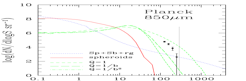
Figure 1: Differential source counts of SCUBA galaxies at 850$\,\mu$m (solid line) compared with counts expected in the case of observations performed with the angular resolution of Planck/HFI for the three models for the evolution of the amplitude of the three-point correlation function, $Q(z)$, (model (i): short dashes; model (ii): long dashes; model (iii): dot-dashed line). The summed contributions from (unclustered) spiral galaxies, starburst galaxies, and extragalactic radio sources is represented by the dotted line. The filled circles with error bars show the counts estimated from the simulations (see text). The vertical dotted line shows the Planck/HFI $5\sigma$ detection limit ($S_{d}=288\,$mJy) estimated by Negrello et al. (2004) allowing for clustering fluctuations.

3 Numerical simulations

To test the reliability of our analytical approach, numerical simulations of sky patches were performed using the fast algorithm recently developed by González-Nuevo et al. (2004). Only SCUBA galaxies were taken into account. Sources were first randomly distributed over the patch area, with surface densities given, as a function of the flux density, by the model of Granato et al. (2004); we have considered sources down to $S_{\rm min}=0.01\,$mJy. Then, the projected density contrast as a function of position, $\delta({\mathbf{x}})$, was derived and its Fourier transform, $\delta({\mathbf{k}})$, was computed. Next, in Fourier space, we added the power spectrum corresponding to the two-point angular correlation function, $w(\theta)$, given by model 2 of Negrello et al. (2004), to the white noise power spectrum corresponding to the initial spatial distribution and obtained the transformed density field of spatially correlated sources. Then we apply the inverse Fourier transform to get the projected distribution of clustered sources in the real space and we associate randomly the fluxes to the simulated sources according to the differential counts predicted by the model of Granato et al. (2004) (for more details, see González-Nuevo et al. 2004)

Simulations were carried out for surveys in:

• the 850$\,\mu$m channel of the High Frequency Instrument (HFI) of the ESA Planck satellite (FWHM=300^′′; Lamarre et al. 2003);

• the 500$\,\mu$m channel of the Spectral and Photometric Imaging REceiver (SPIRE) of the ESA Herschel satellite (FWHM=34.6^′′; Griffin et al. 2000).

In the Planck/HFI case, we have simulated sky patches of $12^{\circ}.8\times 12^{\circ}.8\,\hbox{deg}^{2}$ with pixels of $1.5\times 1.5\,\hbox{arcmin}^{2}$. In the Herschel/SPIRE case the patches were of $3^{\circ}.28\times 3^{\circ}.28\,\hbox{deg}^{2}$ and the pixel size was $1/3$ of the FWHM.

To check the simulation procedure we have compared the confusion noise, $\sigma$, obtained from them with the analytical results by Negrello et al. (2004). In the case of Planck/HFI, from the simulations we get $\sigma_{P}=20\,$mJy and $\sigma_{C}=50\,$mJy for Poisson distributed and clustered sources, respectively, in very good agreement with the analytic results, $\sigma_{P}=20\,$mJy and $\sigma_{C}=53\,$mJy. For the Herschel/SPIRE channel the simulations give $\sigma_{P}=6.4\,$mJy and $\sigma_{C}=1.2\,$mJy, to be compared with $\sigma_{P}=6.0\,$mJy and $\sigma_{C}=3.2\,$mJy obtained by Negrello et al. (2004). The apparent discrepancy of the results for $\sigma_{C}$ actually corresponds to the uncertainty in this quantity, very difficult to determine from the simulations when Poisson fluctuations dominate.

Note that for the very steep counts predicted by the Granato et al. (2004) model, that accurately matches the SCUBA and MAMBO data, both the Poisson and the clustering fluctuations, for the angular resolutions considered here, are independent of the flux limit. We have checked that the results obtained from simulations are independent of the pixel size used.

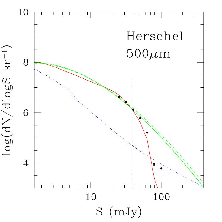
Figure 2: Left-hand panel: same as in Fig. 1 but for the 500$\,\mu$m channel of Herschel/SPIRE. The results for models (ii) and (iii) for the evolution of $Q(z)$ overlap, while model (i) is only slightly higher. Right-hand panel: ratio between the differential counts of SCUBA galaxies estimated from the simulations for the Herschel/SPIRE resolution and those predicted by the model of Granato et al. (2004). The dotted vertical line, in both panels, corresponds to the $5\sigma$ detection limit ($S_{d}=39\,$mJy) estimated by Negrello et al. (2004) accounting also for clustering fluctuations.

4 Results and discussion

The results for the Planck/HFI 850$\,\mu$m channel are shown in Fig. 1, where the solid line gives the counts of SCUBA galaxies predicted by the physically grounded model of Granato et al. (2004), and the dotted line gives the summed counts of spiral and starburst galaxies, and of extragalactic radio sources. For the redshift-dependent luminosity functions of spiral and starburst galaxies we have adopted the same phenomenological models as in Negrello et al. (2004), while for radio galaxies we have used the model by De Zotti et al. (2004). The short-dashed, long-dashed, and dot-dashed lines show the counts of “clumps” expected from our analytic formalism for the three evolution models of the amplitude $Q$ of the three-point correlation function. As expected, at the Planck/HFI resolution the counts of “clumps” are sensitive to the evolution of the three-point correlation function. Clearly the predicted counts below $\simeq 50\,$mJy, where Poisson fluctuations become important, are of no practical use; they are shown just to illustrate how the formalism accounts for the disappearance of lower luminosity objects which merge into the “clumps”.

The filled circles with error bars in Fig. 1 are obtained filtering the simulated maps with a Gaussian response function of 5^′ FWHM to mimic Planck/HFI observations. The lower flux limit of the estimated counts is set by Poisson fluctuations. It should be noted that the procedure used for the simulations takes into account only the two-point angular correlation function and does not allow us to deal with the three-point correlation function and with its cosmological evolution, which are included in the analytic model. In principle it is possible to go the other way round, i.e. to evaluate from the simulations the reduced angular bispectrum, $b_{r}$, by applying the standard Fourier analysis (González-Nuevo et al. 2004; Argüeso et al. 2003) and infer from it an estimate of the three-point correlation function weighted over the redshift distribution. However, the relationship of the three-point correlation function with the angular bispectrum is through a six dimensional integral which is really difficult to deal with in practice (Szapudi 2004). An alternative possibility consists in computing the number of triplets (above a fixed flux threshold) and in using the estimator developed by Szapudi $\&$ Szalay (1998) to derive an estimate of the three-point angular correlation function. On the whole, these methods turn out to be impractical to take into account also the effect of the evolving three-point correlation function when comparing simulations with analytic results. On the other hand, it is very reassuring that the counts obtained from simulations are within the range spanned by analytic models.

In the Herschel case, the beam encompasses only a small fraction of the “clump” and therefore the observed flux is generally dominated by the single brightest source in the beam. Thus, the analytic model described in Section 2 is no longer applicable. As illustrated by the left-hand panel of Fig. 2, such formalism would strongly over-predict the observed counts at bright flux densities (and the results are essentially independent of the three-point correlation function). On the other hand, the simulations (filled circles with error bars) show that neighbour sources appreciably contribute to the observed fluxes, hence to the counts at bright flux density levels, as more clearly illustrated by the right-hand panel of Fig. 2. Such count estimates were obtained filtering the simulated maps with a Gaussian response function of FWHM=34.6^′′, appropriate for the Herschel $500\,\mu$m channel; again, the lower flux limit of the estimated counts is set by Poisson fluctuations.

5 Conclusions

Theoretical arguments and observational data converge in indicating that the very luminous (sub)-mm sources detected by SCUBA and MAMBO surveys are highly clustered (clustering radius $r_{0}\simeq 8\hbox{h}^{-1}\,$Mpc). On the other hand, the limited sizes of telescopes of forthcoming space instruments operating in the sub-mm domain, such as Planck/HFI and Herschel/SPIRE, imply relatively poor angular resolutions ($\hbox{FWHM}\simeq 5^{\prime}$ for Planck at $850\,\mu$m, and $\simeq 34.6^{\prime\prime}$ for Herschel at at $500\,\mu$m).

In the Planck/HFI case the summed fluxes of physically correlated sources within the beam are generally higher than the luminosity of the brightest source in the beam, so that the outcome of the surveys will be counts of “clumps” of sources rather than of individual sources. We have argued that the luminosity distribution of such “clumps” at any redshift can be modelled with a log-normal function, with mean determined by the average source luminosity and by the average of summed luminosities of neighbours, and variance made of three contributions (the variances of source luminosities, of neighbour luminosities, and of neighbour numbers). The latter contribution depends on the three-point correlation function, so that the counts of “clumps” provide information on this elusive quantity and on its cosmological evolution. Under the, rather extreme, assumption that the coefficient, $Q$, of the three-point correlation function is independent of redshift, the counts of “clumps” extend beyond the formal $5\sigma$ detection limit. In the more likely cases of $Q$ decreasing as $b^{-1}$ or $b^{-2}$, $b$ being the bias factor, the “clumps” will only show up in Planck maps as $<5\sigma$ fluctuations. Anyway, the Planck surveys will provide a rich catalogue of candidate proto-clusters at substantial redshifts (typically at $z\simeq 2$–3), very important to investigate the formation of large scale structure and, particularly, to constrain the evolution of the dark energy thought to control the dynamics of the present day universe. Detailed numerical simulations carried out using the fast algorithm recently developed by González-Nuevo et al. (2004) are fully consistent with the analytic results, although a full comparison would require an upgrade of the algorithm to include the effect of the evolving three-point correlation function.

As the ratio of the beam-width to the clustering angular size decreases, the observed fluxes approach those of the brightest sources in the beam and the “clump” formalism no longer applies. However, simulations show that also in the case of the Herschel/SPIRE $500\,\mu$m survey the contribution of neighbours to the observed fluxes enhances the bright tail of the observed counts. Due to the extreme steepness of such tail, as predicted by the model of Granato et al. (2004), even a modest addition to the fluxes of the brightest sources may lead to counts at flux densities $\simeq 100\,$mJy several times higher than would be observed with a high resolution instrument. It should be noted that, in the case of strong clustering, the canonical $5\sigma$ detection limit (shown by the vertical dotted line in both panels of Fig. 2) does not frees the observed counts from the confusion bias.

References

- [\citeauthoryearArgüeso, González-Nuevo, & Toffolatti2003] Argüeso F., González-Nuevo J., Toffolatti L., 2003, ApJ, 598, 86
- [Bernardeau 1994 1994] Bernardeau F., 1994, A&A, 291, 697
- [Bernardeau 1992 1992] Bernardeau F., Schaeffer R., 1992, A&A, 255, 1
- [Bernardeau 1999 1999] Bernardeau F., Schaeffer R., 1999, A&A, 349, 697
- [\citeauthoryearBlain2001] Blain A.W., 2001, Proc. of the ESO7ECF/STScI workshop, S. Cristiani, A. Renzini, R.E. Willians eds., Springer, p. 129
- [Blain et al. 2004] Blain A.W., Chapman S.C., Smail I., Ivison R., 2004, ApJ, in press, astro-ph/0405035
- [Coles, Jones 1991] Coles P., Jones B., 1991, MNRAS, 248, 1
- [Colombi et al. 1996 1996] Colombi S., Bouchet F.R., Hernquist L., 1996, ApJ, 465, 14
- [Condon 1974 1974] Condon J.J., 1974, ApJ, 188, 279
- [De Zotti et al. 1996 1996] De Zotti G., Franceschini A., Toffolatti L., Mazzei P., Danese L., 1996, ApL&C, 35, 289
- [] De Zotti G., Ricci R., Mesa D., Silva L., Mazzotta P., Toffolatti L., González-Nuevo J., 2004, A&A, in press
- [Eales et al. 2000 2000] Eales S., Lilly S., Webb T., Dunne L., Gear W., Clements D., Yun M., 2000, AJ, 120, 2244
- [\citeauthoryearEddington1913] Eddington A.S., 1913, MNRAS, 73, 359
- [\citeauthoryearFry 1984] Fry J.N., 1984, ApJ, 279, 499
- [\citeauthoryearFry, Gaztañaga 1993] Fry J.N., Gaztañaga E., 1993, ApJ, 413, 447
- [\citeauthoryearFry et al. 1993] Fry J.N., Melott A., Shandarin S.F., 1993, ApJ, 412, 504
- [\citeauthoryearFry, Seldner 1982] Fry J.N., Seldner M., 1982, ApJ, 259, 474
- [\citeauthoryearGaztañaga, Bernardeau 1998] Gaztañaga E., Bernardeau F., 1998, AA, 331, 829
- [] González-Nuevo, J., L. Toffolatti, and F. Argüeso (2004). ApJ, in press, (astro-ph/0405553).
- [Granato et al. 2004] Granato G.L., De Zotti G., Silva L., Bressan A., Danese L., 2004, ApJ, 600, 580
- [Griffin et al. 2000] Griffin M.J., Swinyard B.M., Vigroux L.G., 2000, Proceedings of the SPIE, 4013, 184
- [Haiman & Knox 2000 2000] Haiman Z., Knox L., 2000, ApJ, 530, 124
- [\citeauthoryearHogg2001] Hogg D.W., 2001, AJ, 121, 1207
- [\citeauthoryearHogg & Turner1998] Hogg D.W., Turner E.L., 1998, PASP, 110, 727
- [Holland et al. 1999] Holland W.S. et al., 1999, MNRAS, 303, 659
- [\citeauthoryearHughes, Gaztañaga2001] Hughes D.H., Gaztañaga E., 2001, Proc. of the conference Deep millimeter surveys: implications for galaxy formation and evolution, J.D. Lowenthal & D.H. Hughes eds., World Scientific Publishing (Singapore), p. 207
- [Jing, Boerner1997] Jing Y.P., Boerner G., 1997, AA, 318, 667
- [Jing, Boerner1998] Jing Y.P., Boerner G., 1998, ApJ, 503, 37
- [\citeauthoryearJing & Boerner2004] Jing Y.P., Boerner G., 2004, ApJ, 607, 140
- [Juszkiewicz et al. 1993] Juszkiewicz R., Bouchet F.R., Colombi S., 1993, ApJ, 412, L9
- [Kayo et al. 2001] Kayo I., Taruya A., Suto Y., 2001, ApJ, 561, 22
- [Kofman et al. 1994 1994] Kofman L., Bertschinger E., Gelb J.M., Nusser A., Dekel A., 1994, ApJ, 420, 44
- [Lahav et al. 2002] Lahav O. et al. (2dFGRS Team), 2002, MNRAS, 333, 961
- [Lamarre et al. 2003] Lamarre J.-M. et al., 2003, Proceedings of the SPIE, 4850, 730
- [Madgwick et al. 2003] Madgwick D.S. et al., 2003, MNRAS, 344, 847
- [Magliocchetti et al. 2001 2001] Magliocchetti M., Moscardini L., Panuzzo P., Granato G.L., De Zotti G., Danese L., 2001, MNRAS, 325, 1553
- [\citeauthoryearMurdoch, Crawford, & Jauncey1973] Murdoch H.S., Crawford D.F., Jauncey D.L., 1973, ApJ, 183, 1
- [Negrello et al. 2004] Negrello M., Magliocchetti M., Moscardini L., De Zotti G., Granato G.L., Silva L., 2004, MNRAS, 352, 493
- [Peacock, Dodds1996] Peacock J.A., Dodds S.J., 1996, MNRAS, 280, L19
- [Peebles 1980] Peebles P.J.E., 1980, The Large-Scale Structure of the Universe, Princeton Univ. Press, Princeton (P80)
- [Peebles, Groth 1975] Peebles P.J.E., Groth E.J., 1975, ApJ, 196, 1
- [Perrotta et al. 2003 2003] Perrotta F., Magliocchetti M., Baccigalupi C., Bartelmann M., De Zotti G., Granato G.L., Silva L., Danese L., 2003, MNRAS, 338, 623
- [Scheuer 1957] Scheuer P.A.G., 1957, Proc. Cambridge Phil. Soc., 53, 764
- [Scoccimarro et al. 1998] Scoccimarro R., Colombi S., Fry J.N., Frieman J.A., Hivon E., Melott A., 1998, ApJ, 496, 586
- [Scott & White 1999 1999] Scott D., White M., 1999, A&A, 346, 1
- [Sheth Tormen 1999] Sheth R.K., Tormen G., 1999, MNRAS, 308, 119
- [Smail et al. 2003 2003] Smail I., Chapman S.C., Blain A.W., Ivison R.J., 2003, proc. of the meeting Maps of the Cosmos ASP Conference Series, M. Colless & L. Staveley-Smith eds., in press (astro-ph/0311285)
- [Smith et al. 2003] Smith R.E. et al., 2003, MNRAS, 341, 1311
- [Spergel et al. 2003 2003] Spergel D.N. et al., 2003, ApJ, 148, 175
- [\citeauthoryearSzapudi2004] Szapudi I., 2004, ApJ, 605, L89
- [Szapudi et al. 1996 1996] Szapudi I., Meiksin A., Nichol R.C., 1996, ApJ, 473, 15
- [Szapudi et al. 2001 2001] Szapudi I., Postman M., Lauer T.R., Oegerle W., 2001, ApJ, 548, 114
- [] Szapudi I., Szalay A. S., 1998, ApJ, 494, L41
- [Takeuchi & Ishii 20042004] Takeuchi T.T., Ishii T.T., 2004, ApJ, 604, 40
- [Taylor et al. 2000 2000] Taylor A.N., Watts P.I.R., 2000, MNRAS, 314, 92
- [Toffolatti et al. 1998] Toffolatti L., Argüeso Gómez F.A., De Zotti G., Mazzei P., Franceschini A., Danese L., Burigana C., 1998, MNRAS, 297, 117