Probing galaxy density profiles with future supernova surveys

Abstract

In this paper we discuss the possibility to measure the Hubble parameter and the slope of galaxy density profiles using future supernova data. With future supernova surveys such as SNAP, large numbers of core collapse supernovae will be discovered, a small fraction of which will be multiply imaged. Measurements of the image separation, flux-ratio, time-delay and lensing foreground galaxy for these systems will provide tight constraints on the slope of galactic halos as well as providing complementary and independent information to other cosmological tests with respect to the Hubble parameter.

1 Introduction

In recent years, precise measurements of the Cosmic Microwave Background (CMB), large scale structure (LSS), and distant supernovae (SNe) have increased our knowledge of the large scale properties of the universe tremendously. The standard $\Lambda$CDM model of cosmology has turned out to be able to fit all available data with only a few free parameters.

However, there are still many parameters related to cosmology which are not well determined by the present large scale observations. For instance, in order for the CMB data from the WMAP experiment (Spergel et al., 2003; Bennett et al., 2003; Kogut et al., 2003; Hinshaw et al., 2003; Verde et al., 2003; Peiris et al., 2003) to provide a stringent limit on the curvature of the universe, a prior on the Hubble parameter is necessary. This degeneracy can be broken by adding LSS data from surveys such as the Sloan Digital Sky Survey (SDSS) (Tegmark et al. 2004a, ; Tegmark et al. 2004b, ) or the 2dF survey (Peacock et al., 2001), but other independent methods for measuring the Hubble parameter precisely are of great interest.

Another problem is that the nature of the dark matter is at present unknown. The properties of dark matter on large scales are compatible with a heavy, collisionless species which clusters gravitationally, cold dark matter (CDM). On the other hand there are significant problems with understanding some properties of galaxies in CDM models. Numerical simulations of galaxy formation in CDM models show that dark matter halos exhibit a universal density profile with a central slope $\rho\propto r^{-\eta}$, with $\eta\simeq 1-1.5$ (Navarro et al., 1996; Ghigna et al., 2000; Power et al., 2003; Fukushige et al., 2004; Hayashi et al., 2003; Kazantzidis et al., 2004; Navarro et al., 2004). At large radii the profile steepens to $\rho\propto r^{-3}$. While the outer slope is consistent with current observations, there are problems with fitting the inner slope of halos.

Observations of rotation curves of many dwarf galaxies, indicating almost constant density cores, suggest that the inner density profiles in these systems are much shallower than found in simulations (de Blok et al., 2001; van den Bosch et al., 2000; Dutton et al., 2003; Simon et al. 2003a, ; Simon et al. 2003b, ). Another problem is that the number of subhalos within a Milky Way-sized halo predicted by the simulations exceed the observed number of satellite galaxies by at least an order of magnitude.

Many explanations have been offered for this discrepancy. One possibility is that tidal interactions between baryons and dark matter erase the central cusps, and that early star formation expels baryons from small subhalos, rendering them invisible. Whether this purely astrophysical explanation can work is not clear at present. Another possibility is that the properties of dark matter are slightly different from pure CDM. If for instance dark matter has relatively strong self-interactions or is warm instead of cold, shallow density profiles and lack of subhalos might be explained. However, it should be noted that the simplest models of self-interacting dark matter predict large constant-density cores in clusters of galaxies which are ruled out by X-ray and gravitational lensing observations (Meneghetti et al. 2001; Arabadjis, Bautz, & Garmire 2002; Dahle, Hannestad, & Sommer-Larsen 2003).

At present the ultra-high resolution simulations of galaxy formation do not include baryons. This in turn means that for regions of galaxies which are baryon dominated the discrepancy might be resolved by a more complete understanding of feed-back from star formation. In dwarf galaxies this effect is unlikely to be dominant, but for the high-mass systems typically investigated with the method proposed here, the regions probed will be dominated by the baryonic component. Therefore the density profile which we derive for the inner parts of galaxies is likely to be dominated by baryonic physics and can therefore not be directly related to either the pure N-body simulations or to the observations of dark matter dominated dwarf galaxies.

Nevertheless it is of great importance to get a precise observational determination of the halo density profiles in order to understand whether the difference between observations and simulations is generic, or specific to some systems.

Gravitational lensing has the potential to give information on both the matter distribution in galaxies as well as the Hubble parameter. More than 40 years ago, Refsdal outlined how it should be possible to measure the Hubble parameter and the mass of a galaxy by measuring the time delay between multiple images of a supernova (SN) lying far behind and close to the line of sight through the lensing galaxy (Refsdal, 1964).

The first observation of gravitational lensing in a cosmological context was made in 1979, when two images of the quasar QSO 0957+651 at $z\sim 1.4$ was observed. For several reasons, it has been difficult to implement Refsdal’s method on this system. Until 1997 it was not possible to precisely determine a time delay for the system, and even then the complexity of the lens system (a brightest cluster galaxy located close to the center of a galaxy cluster) has made estimates of the Hubble parameter highly uncertain (Keeton et al., 2000). Studies of this system have also showed the importance of including effects from substructure in the lens.

To date, approximately 70 multiply imaged sources have been observed out of which there are eleven firm time delay measurements (Davis et al., 2003; Kochanek & Schechter, 2003;
York et al., 2004). There is not yet any agreement on the correct value of the Hubble parameter inferred from these measurements due to differences in the modeling of the lensing galaxies. In general, modeling the lenses as more concentrated gives larger values of $h$ and vice versa, e.g., Kochanek (2002) obtains $h\sim 0.48^{+0.07}_{-0.04}$ if the lenses have isothermal mass distributions and $h\sim 0.71\pm 0.06$ if they have constant mass-to-light ratio.

There are basically two different routes in trying to improve on current results. One is to try to do extremely careful modeling of single simple lens systems. Following this approach, Wucknitz, Biggs, & Browne (2004) find $h=0.78\pm 0.06$ (2 $\sigma$) based on the lens system B0218+357, consistent with the local estimate $h=0.71\pm 0.06$ (1 $\sigma$) from the Hubble Space Telescope (HST) key project (Mould et al. 2000; Freedman et al. 2001). Another possibility is to combine results from a larger number of, perhaps less well constrained, systems. In this paper, we will investigate the latter method.

In order to avoid any systematic bias due to selection effects, it is important to have a well-defined statistical sample. The currently largest survey of strong lensing events is the recently completed Cosmic Lens All-Sky Survey. A subsample of 8958 flat-spectrum radio sources of which 13 have multiple images constitutes a well-defined statistical sample and has been used to constrain cosmological parameters as well as galaxy properties (Davis et al., 2003; Chae et al., 2004).

Future surveys that will improve statistics and also include multiply imaged SNe for which time delay measurements can be obtained at high accuracy due to the characteristic light curves include Pan-STARRS and the Supernova Acceleration Probe (SNAP) .

In this paper we investigate how future SNAP data of multiply imaged core-collapse SNe can be used to measure the slope of galactic halos and the Hubble parameter (see also Holz, 2001; Oguri et al., 2003). This paper extends and generalizes earlier work
(Goobar et al. 2002a, ) where similar data was used to constrain $h$ and $\Omega_{\rm M}$ using simpler lens models. A recent work by Oguri & Kawano (2003) have considered a similar use of quadruply lensed Type Ia SNe events. The possiblity of using SNe that are multiply lensed by rich galaxy clusters to constrain $h$ has been considered by Bolton & Burles (2003). The complementarity of strong lensing to other probes of the expansion rate is discussed by Linder (2004).

Finally, it should be noted that while the method proposed here is very sensitive to the inner density profile of galaxies, this density profile does not necessarily reflect the nature of pure dark matter halos. Lensing mainly occurs in relatively massive galaxies in which baryonic material is a dominant component at small radii. This in turn means that there can be a substantial modification of the inner density profile due to cooling and infall (Kochanek & White, 2001).

In Sec. 2, we describe the lens model used in the simulations and analysis and in Sec. 3 we describe our numerical simulations. Errors are discussed in Sec. 4 and our results are presented in Sec. 5. Finally, Sec. 6 contains a summary of our results.

2 Method

2.1 Lens model

For most lensing purposes, galaxy matter distributions can be described by the projected Newtonian gravitational potential

$$\Psi=\frac{2D_{l}D_{ls}}{c^{2}D_{s}\xi_{0}^{2}}\int\Phi dl.$$ (1)

We assume that lens systems are characterized by a simple power-law density profile

$$\rho(r)\propto r^{-\eta}.$$ (2)

This is not a good approximation at all radii since the slope is expected to change with radius. In practice however, almost all images of multiply lensed SNe are at a limited range of small $r$ (see Fig. 1) and thus only the inner slope is probed and the single power-law density profile is an excellent approximation.

For the power-law density profile, the lenses can be described by the projected potential

$$\Psi=\frac{x_{E}^{\eta-1}}{3-\eta}x^{3-\eta}$$ (3)

where $x$ is the impact parameter (in arbitrary units, $\xi_{0}$) and $x_{E}$ is the Einstein radius.

2.2 Time delay

The time delay for a gravitationally lensed image as compared to an undeflected image is in the general case given by (Schneider et al. 1992)

$$T=\frac{\xi_{0}^{2}D_{s}}{D_{l}D_{ls}}(1+z_{l})\left[\frac{({\bf x}-{\bf y})^{2}}{2}-\Psi\right],$$ (4)

where $\xi_{0}$ is the (arbitrary) scale length, the $D$’s are angular diameter distances and $y$ is the source position. The time delay between two lensed images is given by $\Delta t=T_{2}-T_{1}$. For an isothermal lens, we have $\eta=2$ and

$$\Delta t_{\rm SIS}=\frac{\xi_{0}^{2}}{2}\frac{D_{s}}{D_{l}D_{ls}}(1+z_{l})(x_{1}^{2}-x_{2}^{2}).$$ (5)

Putting $\xi_{0}=D_{l}$, i.e., denoting positions in terms of angles we get

$$\Delta t_{\rm SIS}=\frac{1}{2}\frac{D_{l}D_{s}}{D_{ls}}(1+z_{l})(\theta_{1}^{2}-\theta_{2}^{2}).$$ (6)

In the general case of $\eta\neq 2$, we can rewrite Eq. (4) in terms of $q\equiv\Delta\theta/<\theta>$ where $\Delta\theta=\theta_{1}-\theta_{2}$ and $<\theta>=(\theta_{1}+\theta_{2})/2$ and Taylor expand to get [after some tedious calculations; see also Kochanek & Schechter (2003) and Chang & Refsdal (1977) for an earlier approximation]

$$\Delta t = \frac{(\eta-1)}{2}\frac{D_{l}D_{s}}{D_{ls}}(1+z_{l})(\theta_{1}^{2}-\theta_{2}^{2})\left[1-\frac{(2-\eta)^{2}}{12}q^{2}+\mathcal{O}(q^{3})\right]$$ (7)

$$\simeq (\eta-1)\Delta t_{\rm SIS}\left[1-\frac{(2-\eta)^{2}}{12}q^{2}\right].$$

We see that we have an almost perfect degeneracy between $\eta-1$ and $h$ (which comes in through the distances). This degeneracy can be broken by including data from the observed flux ratio.

2.3 Flux ratio

We denote the flux ratio $r\equiv\mu_{1}/|\mu_{2}|$. The magnification $\mu$ for a source at position $y$ observed at position $x$ is given by

$$|\mu|=\left|\frac{x}{y}\frac{dx}{dy}\right|.$$ (8)

Computing the lensing angles through $\alpha=\nabla\Psi$ and using the lens equation

$$y=x_{1}-\alpha_{1}=x_{2}-\alpha_{2}\,,$$ (9)

we can express the flux ratio as

$$r = \left|\frac{x_{1}}{x_{2}}\right|\left|\frac{1-(2-\eta)x_{2}^{1-\eta}(x_{1}+x_{2})/(x_{1}^{2-\eta}+x_{2}^{2-\eta})}{1-(2-\eta)x_{1}^{1-\eta}(x_{1}+x_{2})/(x_{1}^{2-\eta}+x_{2}^{2-\eta})}\right|$$ (10)

$$= r_{\rm SIS}\left|\frac{1-(2-\eta)x_{2}^{1-\eta}(x_{1}+x_{2})/(x_{1}^{2-\eta}+x_{2}^{2-\eta})}{1-(2-\eta)x_{1}^{1-\eta}(x_{1}+x_{2})/(x_{1}^{2-\eta}+x_{2}^{2-\eta})}\right|.$$

Expanding this to second order in $q$, we obtain

$$r\simeq 1+(\eta-1)q+\frac{1}{2}(\eta-1)^{2}q^{2}+{\cal O}(q^{3}).$$ (11)

Eqns. (7) and (11) are excellent approximations for small $q$ and/or $\eta\sim 2$. In order to show the general parameter dependencies, we generalize in the following the expanded expressions to include also the effects from ellipticities and external shear. However, in the subsequent $\chi^{2}$-analysis, we use the full expressions for the time delay and the flux ratio to avoid any bias due to the Taylor expansion.

2.4 Ellipticity

In order to treat possible non-sphericity of the lens systems we add a quadrupole term to the projected potential, $\Psi$,

$$\Psi=\Psi_{0}\left(1+a\cos 2\phi\right),$$ (12)

where $\Psi_{0}$ is the spherical potential given in Eq. (3) and $\phi$ is the angle of the image relative to the quadrupole axis. Using this potential it is possible to derive an analytic expression for the time delay, which is, however, quite complicated. If the system is assumed to have relatively small ellipticity, an assumption already implicit in the fact that we represent the asphericity of the lens with a quadruple moment, then the angle of the second image can be written as a function of the first

$$\phi_{2}=\phi_{1}+\pi-\delta,$$ (13)

where $\delta$ is a small parameter (and explicitly 0 for spherical systems). We expand the time delay in the parameters $q$ and $\delta$ to find

$$\Delta t\simeq(\eta-1)\Delta t_{\rm SIS}\left[1-\frac{(\eta-2)^{2}}{12}q^{2}-\frac{\eta-2}{4}\delta^{2}\right],$$ (14)

an expression which is valid to second order in both $q$ and $\delta$. In the same way it is possible to derive an expression for the flux ratio of a system with a quadrupole moment. To second order in $q$ and $\delta$ we find that

$$r = 1+2\delta\cot(2\phi_{1})+\frac{3+\cos(4\phi_{1})}{\sin^{2}(2\phi_{1}^{2})}\delta^{2}$$ (15)

$$\,\,+(\eta-1)\left[1+\delta\cot(2\phi_{1})\right]q+\frac{1}{2}(\eta-1)^{2}q^{2}+{\cal O}(q^{3},\delta^{3},q^{2}\delta,q\delta^{2}).$$

The above expression appears divergent for $\phi_{1}\to 0$ because of the $1/\sin(2\phi_{1})$ terms. However, since $\delta\to 0$ when $\phi_{1}\to 0$, the quantity $\delta/\sin(2\phi_{1})$ remains finite, and there are no actual divergences.

2.5 External shear

Most lens systems are embedded within an external potential which gives rise to an additional shear contribution. Following Kochanek & Schechter (2003) we write the combined potential as

$$\Psi=\Psi_{0}\left(1+a\cos 2\phi\right)+\gamma_{\rm ext}r^{2}\cos[2(\phi-\phi_{0})],$$ (16)

where $\phi-\phi_{0}$ is the angle between the image position and the quadrupole axis of the external potential. If the external shear is aligned with the lens system itself then $\phi_{0}=0$, but in the general case $\phi_{0}\neq 0$.

Since $\gamma$ should be small in order to justify treating the external potential as a quadrupole (an assumption supported in, e.g., Dalal & Watson, 2004), we derive expressions for $\Delta t$ and $r$ which are valid to second order in $q$, $\delta$ and $\gamma$ for arbitrary values of $\phi_{0}$. The expressions we find are

$$\Delta t\simeq(\eta-1)\Delta t_{\rm SIS}\Big{[}1-\frac{(\eta-2)^{2}}{12}q^{2}+\delta\gamma+\frac{1}{4}\delta^{2}(\eta-2)\Big{]}$$ (17)

and

$$r \simeq 1+(\eta-1)q+2\delta\cot(2\phi_{1})+\frac{1}{2}\left[q(\eta-1)+2\delta\cot(2\phi_{1})\right]^{2}$$

$$+\frac{\gamma^{2}}{8(\eta-1)\sin(\phi_{1})^{2}\cos(\phi_{1})^{2}}\Bigg{[}\Big{(}\eta(10+\eta)-43\Big{)}\cos(4\phi_{0})+(\eta-1)^{2}\cos[4(\phi_{0}-2\phi_{1})]$$

$$+2[23+(\eta-8)\eta-(\eta-3)(\eta-1)\cos[4(\phi_{0}-\phi_{1})]-(\eta^{2}-1)\cos(4\phi_{1})]\Bigg{]}$$

$$-\frac{8\gamma\cos(\phi_{0})\sin(\phi_{0})}{\sin(\phi_{1})\cos(\phi_{1})}-\frac{\gamma}{16(\eta-1)}\Bigg{[}16\delta(\eta-1)^{2}\cos(2\phi_{0})\sin(2\phi_{1})$$

$$+\frac{\sin(2\phi_{0})}{\sin(\phi_{1})^{2}\cos(\phi_{1})^{2}}\Big{(}-\delta[81+(\eta-98)\eta]\cos(2\phi_{1})+(\eta-1)[\delta(\eta-1)\cos(6\phi_{1})+8q\eta\sin(2\phi_{1})]\Big{)}\Bigg{]}.$$

3 Simulated data

With the proposed SNAP satellite a large number of core collapse supernovae (CC SNe) will be discovered, of which a small fraction will be multiply imaged. We use the SNOC package (Goobar et al. 2002c, ) to simulate a total of $1.1\cdot 10^{6}$ CC SNe, the predicted number following the prescriptions in Dahlén & Fransson (1999) for a 20 square degree field during three years for $z<5$. Lensing effects are investigated by ray-tracing using SIS halo profiles since lensing statistics are insensitive to ellipticities and shear (Huterer, 2004). We derive a galaxy mass function by combining the Schechter luminosity function with a mass-to-luminosity relation for fundamental plane ellipticals; see Bergström et al. (2000) for details.

The cosmology used is $h=0.65$, $\Omega_{\rm M}=0.3$ and $\Omega_{\rm\Lambda}=0.7$. Out of the $1.1\cdot 10^{6}$ CC SNe, 2613 have multiple images [this is the sample used in Goobar et al. (2002a)]. Out of these, 857 have either an I-band or J-band peak brightness $<28.5$ mag for the dimmest image. In order to avoid contamination from the lens galaxy in the SN detection, we impose a constraint that the surface brightness of the lens galaxy has to be fainter than 24 I magnitudes per square arcsecond. We assume that the lens galaxies follow a de Vaucouleurs profile (de Vaucouleurs, 1948)

$$I(r)=I_{e}\exp\left\{-7.67\left[(r/r_{e})^{1/4}-1\right]\right\}$$ (19)

where $I(r)$ is the surface brightness at radius $r$, $r_{e}$ is the half light radius and $I_{e}$ is the surface brightness at $r_{e}$. Observationally, the surface brightness at $r_{e}$ (in B magnitudes per square arcsecond), $\mu_{Be}$, can be related to the half light radius according to (Kormendy, 1977)

$$\mu_{{\rm B}e}=3.02\log(r_{e}/{\rm 1\,kpc})+19.74.$$ (20)

The absolute B-band magnitude, $M_{\rm B}$, can be written

$$M_{\rm B}=\mu_{{\rm B}e}-5\log(r_{e}/{\rm 1\,kpc})-39.28.$$ (21)

We use Eqns. (19)-(21) together with the Faber-Jackson relation $L\propto v^{4}$ and a K-correction appropriate for early-type galaxies to calculate the I-band surface brightness, $\mu_{\rm I}$ at the position of the faintest image. Here, we have neglected the modest surface brightness evolution of elliptical galaxies to $z\sim 1$. All but 4 of the 857 SNe satisfy $\mu_{\rm I}>24$ at this position and we conclude that the lens galaxy light does not significantly affect the SN observations.

Since we assume fairly clean and simple lens systems in our analysis, we incorporate a quality factor, $f$, giving the fraction of the lens systems that fulfill our requirements of a single dominant deflector with not too large ellipticity or external shear. In accordance with currently observed systems (see, e.g., Kochanek & Schechter 2003), we set $f=0.5$ in our analysis. We also perform an extremely conservative analysis setting $f=0.05$.

Even though we can derive fair lensing statistics using a simple SIS galaxy profile, it is important to include lens ellipticities and galaxy environments in the analysis
(Keeton & Zabludoff, 2004). We modify our simple simulated lensing systems by adding the effects of ellipticities and shear according to the distributions described in Sec. 4. Since we expect a scatter in the properties of individual halos, we have also added a 1 sigma dispersion in the value of $\eta$ for individual halos of $\Delta\eta=0.2$. However, in order to constrain the mean slope of galactic halos, we are still fitting $\eta$ as a global parameter.

4 Assumed errors

$\sigma_{r}$:

Errors in the flux ratio of the two SN images will be dominated by the effects of microlensing by compact objects (Schneider & Wagoner 1987) and millilensing by cold dark matter (CDM) sub-halos (Dalal & Kochanek 2002; Keeton 2003; Mao et al. 2004), rather than flux measurement uncertainties.

In QSO microlensing, a source of essentially constant size is observed moving across a microlens amplification pattern at a typical transverse velocity of $\sim 500\,{\rm km\,s}^{-1}$. In the case of microlensing of a SN, this transverse velocity is dwarfed by the $\sim 10^{4}\,{\rm km\,s}^{-1}$ expansion velocity of the SN photosphere. If the center of the SN is close to a critical line, an amplification of several magnitudes may result from microlensing (Schneider & Wagoner 1987). In this case, the shape of the light curve of the affected SN image is usually strongly modified, and such cases should be readily identifiable from a comparison of the light curves of the two SN images.

The light curves of QSO 2237+0305 (Huchra’s lens) presented by the OGLE team
(Wozniak et al., 2000) indicate a scatter $\sigma_{r}=0.4$ caused by stellar microlensing. When also taking into account a $\sim 20\%$ uncertainty in the image fluxes due to CDM substructure, we arrive at a conservative estimate of $\sigma_{r}/r=0.5$, which was used for our simulations.

$\sigma_{\theta}$:

Following Goobar et al. (2002a), we conservatively estimate a positional uncertainty of $\sigma_{\theta}=0.01^{\prime\prime}$ for SNAP data. While millilensing by CDM sub-halos may affect the flux ratio, its effect on image positions would likely be negligible, compared to the measurement uncertainty.

$\Delta t$:

The estimated measurement uncertainty for the time delay is 0.05 days (Goobar et al. 2002a). However, in the presence of microlensing, the measured time delay may depart significantly from the time delay predicted by our smooth macro-lens model. In the most extreme cases, a high-amplification microlensing event may shift the observed maximum by several days (Schneider & Wagoner 1987), but as noted above, such rare events should be identifiable and can thus be removed from the sample of events. We model the observed SN light curve as the intrinsic curve superposed on a smooth gradient, with a typical value similar to the microlens light curves of Wozniak et al. (2000). From this, we estimate an uncertainty $\sigma_{\Delta t}$ of 0.15 days.

$\gamma_{\rm ext}$:

Using N-body simulations and semi-analytic models of galaxy formation, Holder & Schechter (2003) estimate a mean external shear at the position of lens galaxies of $\gamma_{\rm ext}=0.058$, with an rms dispersion of 0.071. They also find a significant tail towards high values of $\gamma_{\rm ext}$. We note that the photometric redshift estimates obtained with SNAP should enable the identification – and removal – of a small subset of lens systems where nearby galaxy groups or clusters produce large values for the external shear.

Quadrupole:

Detailed models of known gravitational lens systems indicate that the mass distribution is aligned with the optical light distribution, with an upper limit $\langle\Delta\phi^{2}\rangle^{1/2}<10\arcdeg$ on the dispersion in the angle between the major axes (Kochanek 2002). The measurement uncertainties in determining the positions of the lensed images with respect to the lens galaxy will be negligible by comparison. In lens galaxies undergoing major mergers, a temporary misalignment of the optical and dark matter may occur (Quadri, Möller & Natarajan 2003). Here, we neglect such effects on the assumption that such merging systems will have morphological and photometric signatures that enable their identification and removal from our sample.

$\sigma_{z_{l}}$:

We adopt $\sigma_{z_{l}}=0.001$ from photometric redshift measurements based on SNAP multi-band photometry (Goobar et al. 2002a).

$\Omega_{m}$:

We use $\Omega_{m}=0.30\pm 0.04$ from the Tegmark et al. (2003b) analysis of SDSS and WMAP data. It should be noted that this is a very conservative estimate of the error. Future CMB measurements from experiments like Planck, as well as large scale weak lensing surveys are likely to increase the precision with which $\Omega_{m}$ can be measured.

5 Results

In order to investigate constraints from the time delay measurements, we perform a $\chi^{2}$-analysis over a $[h,\eta]$-grid

$$\chi^{2}(h,\eta)=[\Delta t_{i}^{\rm exp}-\Delta t_{i}^{\rm th}(h,\eta)]V_{ij}^{-1}[\Delta t_{j}^{\rm exp}-\Delta t_{j}^{\rm th}(h,\eta)],$$ (22)

where $\Delta t_{i}^{\rm exp}$ is the experimental time delays (simulated using the SIS profile and modified to include the effects from ellipticity, external shear and a scatter in the slope, see Sec. 3) and $\Delta t_{i}^{\rm th}(h,\eta)$ is the theoretical time delays. $V_{ij}$ is the error (covariance) matrix. We expect a close to perfect degeneracy between $h$ and $1-\eta$ that can be broken by including information from the flux ratio that is sensitive to the slope $\eta$ only. For constraints using the flux ratio, we use

$$\chi^{2}(h)=[r_{i}^{\rm exp}-r_{i}^{\rm th}(\eta)]V_{ij}^{-1}[r_{j}^{\rm exp}-r_{j}^{\rm th}(\eta)],$$ (23)

where $r_{i}^{\rm exp}$ is the experimental (simulated) flux ratio and $r_{i}^{\rm th}(\eta)$ is the theoretical flux ratio.

In order to avoid any bias due to the second order expansion in $q$ in the time delay and flux ratio, we use the full expression for these quantities. However, since $\eta\sim 2$ in our simulations, the use of Eqns. (17) and (2.5) for the theoretical time delay and flux ratio, respectively, gives close to identical results.

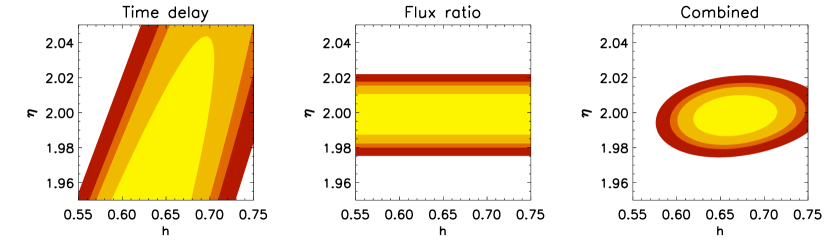
In Fig. 4, results from the time delay (left panel), flux ratio (middle panel) and the combined results (right panel) are shown. Using a quality factor $f=0.5$, this gives a total of $\sim 400$ SNe for the magnitude cuts described in Sec. 3. Contours correspond to 68.3 %, 90 %, 95 % and 99 % confidence levels. It is clear that when combining the results from the time delay and flux ratio measurements, we are able to make a determination of $h$ within 10 % and, perhaps more interestingly, to determine $\eta$ at the per cent level at 95 % confidence.

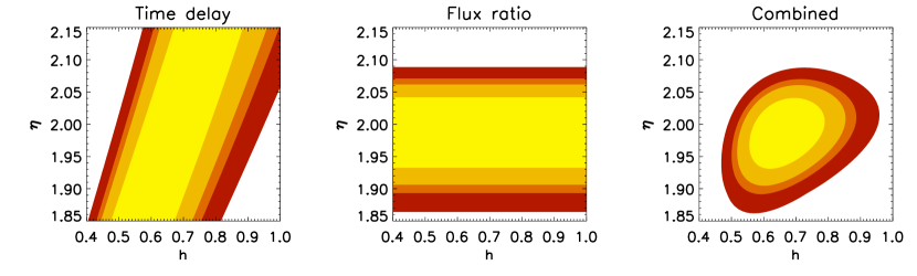
In Fig. 5, results using a quality factor $f=0.05$, giving a total of $\sim 40$ SNe are shown. Even with this drastic decrease in statistics, we are still able to determine the slope $\eta$ to an impressive accuracy.

Constraints from the time delay are almost fully determined by the quality of the time delay measurements whereas the flux ratio constraints are quite robust to all observational errors. Even when increasing the error in the flux ratio observation with a factor of 3 (to 150 %), we are still able obtain $\eta=2\pm 0.06$ at 90 % confidence. Increasing the size of the external shear by a factor of ten causes a systematic bias in the determination of $\eta$ of $\eta=2\rightarrow 1.65$. Increasing the value of the dispersion in the value of $\eta$ for individual halos to $\Delta\eta=0.5$ will cause a bias in $h$ of $h=0.65\rightarrow 0.55$ but the mean slope $\eta$ will still be well-determined. Thus, we conclude that our results are fairly robust even to quite significant changes in the quality and quantity of the data used in the analysis.

As is evident from Eq. (2.5), the effect on the flux ratio from varying $\eta$ is strongest for high $q$, i.e, large flux ratios. For large $q$, we also have large time delays. Since these systems have smaller fractional time delay errors, we obtain stronger constraints also from the time delay analysis for large $q$. Thus, we conclude that systems with large flux ratios and time delays (i.e., large $q$) are very important when constraining galaxy density profiles and the Hubble parameter using strong gravitational lensing. This is confirmed by dividing the lens system into two classes with $0<q<1$ and $1<q<2$ where (for an equal number of lens systems) the class with high $q$ gives confidence contours a factor of $\sim 2$ smaller in the $h$-direction and a factor of $>5$ smaller in the $\eta$-direction compared with the low-$q$ systems.

In practice, it should be possible to obtain additional constraints for a significant fraction of the observed lens systems, since some of the SN host galaxies will be lensed into multiple, resolved images that may be detectable in deep combined frames from the survey. We make no attempt here to model the possible improvements in the parameter determination resulting from such additional constraints, but note that our results here correspond to a pessimistic scenario where no multiply lensed SN host galaxies are detectable.

6 Summary

We have analyzed how the measurement of strongly lensed SNe by future SN surveys will allow for a very precise determination of statistical properties of the matter distribution in galaxies, as well as the Hubble parameter.

Understanding the properties of dark matter in details is one of the most important problems in modern cosmology, and one of the best laboratories for this is galactic halos. While CMB and LSS data probe properties of dark matter on very large scales, measurements of galactic halos probe small scale properties of dark matter, such as free-streaming, dark matter self-interactions (Spergel & Steinhardt, 2000; Dave et al., 2001; Hannestad, 1999; Wandelt et al., 2001; Colin et al., 2002; Burkert, 2000; Firmani et al., 2000; Yoshida et al., 2000), dark matter - baryon interactions (Chen et al., 2002; Boehm et al., 2002), or modified primordial power spectra (Kamionkowski & Liddle, 2000; Sigurdsson & Kamionkowski, 2004).

While the method proposed here is not directly applicable to dwarf galaxies where dark matter properties can be probed directly it allows for a very precise determination of the density profiles of massive galaxies. This in turn can shed light on the feedback between baryons and dark matter during the epoch of non-linear structure formation.

We estimate that with future data it will be possible to constrain the inner density profiles of galactic halos to an accuracy of 1-2%, much better than any present measurement. Furthermore our proposed method mainly probes lens systems at relatively high redshift, $z\gtrsim 1$, where no other reliable method for measuring galaxy density profiles is available.

The estimated precision is based on a sample of roughly 850 multiply imaged SNe. Even with a significantly smaller set of SNe, tight constraints could be obtained. This means that properties like redshift evolution of density profiles, variations in density profiles with galaxy luminosity, color and many other important parameters can be measured by dividing the lens systems into different categories. This in turn will provide valuable information on the physics of galaxy formation.

Figure 1: Distribution of impact parameters for primary images for the lens systems used in the analysis in this paper.

Figure 2: Left panel: The number of observed multiply imaged SNe as a function of magnitude threshold for the dimmest image in the I-band or J-band. Right panel: The solid line shows the distribution of source redshifts, the dotted line the lens redshifts for the sample of 853 SNe that have either an I-band or J-band peak brightness $<28.5$ mag for the dimmest image and host galaxy surface brightness $\mu_{\rm I}>24$ mag at the position of this image.

Figure 3: Upper left: The time delay distribution for 853 SNe that have either an I-band or J-band peak brightness $<28.5$ mag for the dimmest image and host galaxy surface brightness $\mu_{\rm I}>24$ mag at this position. Upper right: The distribution of flux ratios for the same sample. Lower left: The distribution of $q$-values. Lower right: The image separation distribution.

Figure 4: Results from the time delay (left panel), flux ratio (middle panel) and the combined results (right panel) using a quality factor $f=0.5$ or $\sim 400$ SNe. Contours correspond to 68.3 %, 90 %, 95 % and 99 % confidence levels.

Figure 5: Results from the time delay (left panel), flux ratio (middle panel) and the combined results (right panel) using a quality factor $f=0.05$ or $\sim 40$ SNe. Contours correspond to 68.3 %, 90 %, 95 % and 99 % confidence levels. Note different axis range from Fig. 4.

References

- Arabadjis, Bautz, & Garmire (2002) Arabadjis, J.S., Bautz, M.W. and Garmire, G.P. 2002, ApJ, 572, 66
- Bennett et al. (2003) Bennett, C.L. et al., 2003, ApJS, 148, 1
- Bergström et al. (2000) Bergström, L., Goliath, M., Goobar, A. and Mörtsell, E. 2000, A&A, 358, 13
- de Blok et al. (2001) de Blok, W.J.G., McGaugh, S.S., Bosma, A. and Rubin, V.C. 2001, ApJ, 552, L23
- Boehm et al. (2002) Boehm, C., Riazuelo, A., Hansen, S.H. and Schaeffer, R., 2002, Phys. Rev. D66, 083505
- Bolton & Burles (2003) Bolton, A. S. & Burles, S. 2003, ApJ, 592, 17
- van den Bosch et al. (2000) van den Bosch, F.C., Robertson, B.E., Dalcanton, J.J. and de Blok, W.J.G. 2000, AJ, 119, 1579
- Burkert (2000) Burkert, A. 2000, ApJ, 534, L143
- Chae et al. (2004) Chae, K., Chen, G., Ratra, B. and Lee, D., 2004, astro-ph/0403256.
- Chang & Refsdal (1977) Chang, K. and Refsdal, S. 1977, in The Evolution of the Galaxies and its Cosmological Implications, IAU Colloquium 37, Éditions du Centre National de la Recherche Scientifique, p. 369-374
- Chen et al. (2002) Chen, X.L., Hannestad, S. and Scherrer, R.J., 2002 Phys. Rev. D65, 123515
- Colin et al. (2002) Colin, P., Avila-Reese, V., Valenzuela O. and Firmani, C., 2002 ApJ, 581, 777
- Dahle, Hannestad, & Sommer-Larsen (2003) Dahle, H., Hannestad, S. and Sommer-Larsen, J. 2003, ApJ, 588, L73
- Dahlén & Fransson (1999) Dahlén, T. and Fransson, C., 1999, A&A, 350, 349
- Dalal & Kochanek (2002) Dalal, N. and Kochanek, C.S. 2002, ApJ, 572, 25
- Dalal & Watson (2004) Dalal, N. and Watson, C.R., 2004, astro-ph/0409483.
- Dave et al. (2001) Dave, R., Spergel, D.N., Steinhardt, P.J. and Wandelt, B.D., 2001 ApJ, 547, 574
- Davis et al. (2003) Davis, A.N, Huterer, D. and Krauss, L.M., 2003, MNRAS, 344, 1029
- Dutton et al. (2003) Dutton, A.A., Courteau, S., Carignan, C. and de Jong, R., 2003, astro-ph/0310001
- Firmani et al. (2000) Firmani, C., D’Onghia, E., Avila-Reese, V., Chincarini, G. and Hernández, X. 2000, MNRAS, 315, L29
- Freedman et al. (2001) Freedman, W.L., et al. 2001, ApJ, 553, 47
- Fukushige et al. (2004) Fukushige, T., Kawai, A. and Makino, J., 2004, ApJ, 606, 625
- Ghigna et al. (2000) Ghigna, S., Moore, B., Governato, F., Lake, G., Quinn, T. and Stadel, J., 2000 ApJ, 544, 616
- (24) Goobar, A., Mörtsell, E., Amanullah, R. and Nugent, P., 2002a, A&A, 393, 25
- (25) Goobar, A., Bergström, L. and Mörtsell, E., 2002b, A&A, 384, 1
- (26) Goobar, A., Mörtsell, E., Amanullah, R., Goliath, M., Bergström, L. and Dahlén, T., 2002c, A&A, 392, 757. Code available at http://www.physto.se/ariel/snoc/
- Hannestad (1999) Hannestad, S., 1999, astro-ph/9912558.
- Hayashi et al. (2003) Hayashi, E. et al. , 2003, astro-ph/0310576.
- Hinshaw et al. (2003) Hinshaw, G. et al., 2003 ApJS, 148, 135
- Holder & Schechter (2003) Holder, G.P. and Schechter, P.L., 2003, ApJ, 589, 688
- Holz (2001) Holz, D. E. 2001, ApJ, 556, L71
- Huterer (2004) Huterer, D., et al., 2004, astro-ph/0405040.
- Kamionkowski & Liddle (2000) Kamionkowski, M. and Liddle, A.R., 2000, Phys. Rev. Lett.84, 4525
- Kazantzidis et al. (2004) Kazantzidis, S., Mayer, L., Mastropietro, C., Diemand, J., Stadel, J. and Moore, B., 2004, ApJ, 608, 663
- Keeton et al. (2000) Keeton, C.R., et al., 2000, ApJ, 542, 74
- Keeton (2003) Keeton, C.R. 2003, ApJ, 584, 664
- Keeton & Zabludoff (2004) Keeton, C.R. and Zabludoff, A.I., 2004, astro-ph/0406060.
- Kochanek (2002) Kochanek, C.S., 2002, astro-ph/0204043.
- Kochanek & Schechter (2003) Kochanek, C.S. and Schechter, P.L., 2003, astro-ph/0306040.
- Kochanek & White (2001) Kochanek, C.S. and White, M., 2001, ApJ, 559, 331
- Kogut et al. (2003) Kogut, A. et al., 2003, ApJS, 148, 161
- Kormendy (1977) Kormendy, J., 1977, ApJ, 218, 333
- Linder (2004) Linder, E. V. 2004, Phys. Rev. D, 70, 043534
- Mao, Jing, Ostriker, & Weller (2004) Mao, S., Jing, Y., Ostriker, J.P. and Weller, J. 2004, ApJ, 604, L5
- Meneghetti et al. (2001) Meneghetti, M., Yoshida, N., Bartelmann, M., Moscardini, L., Springel, V., Tormen, G. and White, S.D.M. 2001, MNRAS, 325, 435
- Mould et al. (2000) Mould, J.R., et al. 2000, ApJ, 529, 786
- Navarro et al. (1996) Navarro, J.F., Frenk, C.S. and White, S.D.M., 1997, ApJ, 490, 493
- Navarro et al. (2004) Navarro, J.F. et al., 2004, MNRAS, 349, 1039
- Oguri & Kawano (2003) Oguri, M. and Kawano, Y. 2003, MNRAS, 338, L25
- Oguri et al. (2003) Oguri, M., Suto, Y., & Turner, E. L. 2003, ApJ, 583, 584
- Peacock et al. (2001) Peacock, J.A. et al., 2001, Nature 410, 169
- Peiris et al. (2003) Peiris, H.V. et al., 2003, ApJS, 148, 213
- Power et al. (2003) Power, C. et al., 2003, MNRAS, 338, 14
- Quadri et al. (2003) Quadri, R., Möller, O., Natarajan, P., 2003, ApJ, 597, 659
- Refsdal (1964) Refsdal, S., 1964, MNRAS, 128, 307
- Schneider & Wagoner (1987) Schneider, P., Wagoner, R.V., 1987, ApJ, 314, 154
- Schneider et al. (1992) Schneider, P., Ehlers, J. and Falco, E.E., Gravitational Lenses (Springer Verlag, Berlin, 1992).
- Sigurdsson & Kamionkowski (2004) Sigurdsson, K. and Kamionkowski, M., 2004, Phys. Rev. Lett.92, 171302
- (59) Simon, J.D., Bolatto, A.D., Leroy, A. and Blitz, L., 2003a, astro-ph/0310193.
- (60) Simon, J.D., Bolatto, A.D., Leroy, A. and Blitz, L., 2003b, ApJ, 596, 957
- Spergel & Steinhardt (2000) Spergel, D.N. and Steinhardt, P.J., 2000, Phys. Rev. Lett.84, 3760
- Spergel et al. (2003) Spergel, D.N. et al., 2003, ApJS, 148, 175
- (63) Tegmark, M., et al. 2004a, ApJ, 606, 702
- (64) Tegmark, M., et al. 2004b, Phys. Rev. D, 69, 103501
- de Vaucouleurs (1948) de Vaucouleurs, G., 1948, Ann. d’Astrophys. 11, 247
- Verde et al. (2003) Verde, L. et al., 2003, ApJS, 148, 195
- Wandelt et al. (2001) Wandelt, B.D., Dave, R., Farrar, G.R., McGuire, P.C., Spergel, D.N. and Steinhardt, P.J., 2001, in Sources and Detection of Dark Matter and Dark Energy in the Universe, Springer-Verlag, Berlin, 263, astro-ph/0006344.
- Wozniak et al. (2000) Wozniak et al., 2000, ApJ, 540, L65
- Wucknitz, Biggs, & Browne (2004) Wucknitz, O., Biggs, A.D. and Browne, I.W.A. 2004, MNRAS, 349, 14
- York et al. (2004) York, T. Jackson, N., Browne, I.W.A., Wucknitz, O. and Skelton, J.E., 2004, astro-ph/0405115.
- Yoshida et al. (2000) Yoshida, N., Springel, V., White, S.D.M. and Tormen, G., 2000, ApJ, 535, L103