Chandra observations of the massive star-forming region S106

We present Chandra observations of the massive star-forming region S106, a prominent H ii region in Cygnus, associated with an extended molecular cloud and a young cluster. The nebula is excited by a single young massive star located at the center of the molecular cloud and the embedded cluster. The prominence of the cluster in the Chandra observation presented here confirms its youth and allows some of its members to be studied in more detail. We detect X-ray emission from the young massive central source S106 IRS 4, the deeply embedded central object which drives the bipolar nebula with a mass loss rate approximately 1–2 orders of magnitude higher than main sequence stars of comparable luminosity. Still, on the basis of its wind momentum flux the X-ray luminosity of S106 IRS 4 is comparable to the values observed in more evolved (main sequence and giant) massive stars, suggesting that the same process which is responsible for the observed X-ray emission from older massive stars is already at work at these early stages.

1 Introduction

The study of regions of recent star formation provides the observational data necessary to address a number of important astrophysical questions, such as the physics of the star formation process, what determines its efficiency, the characterization of the initial mass function, the stellar chemical evolution and the galactic chemical recycling process; in particular, massive stars, with their strong winds and short lifetime have a strong impact on the circumstellar environment. The high density of absorbing material makes optical observations poorly suited for the observation of the earliest stages of star formation, while the infrared (IR) bands $J,H$ and $K$ have proven to be an excellent tool for unveiling embedded star formation regions due to the reduced impact of dust extinction at longer wavelengths.

A role similar to IR observations is currently being played by X-ray observations, to which dust is as transparent. Given that X-ray luminosity of stars evolves strongly with age, young stars are very active X-ray sources, so that they can be easily selected from field stars. X-ray surveys of young associations and clusters also provide valuable information on the magnetic activity of young stars and on their accretion rates, as well as effectively supplement other approaches to membership determination in these regions (see e.g. Feigelson & Montmerle, 1999, although the field is evolving rapidly). In comparison with the low-mass domain X-ray observations of massive star-forming regions and massive young stellar objects (YSOs) have been been rare, with very few detections of X-ray emission from massive YSOs reported to date (Kohno et al., 2002).

Recently Le Duigou & Knödlseder (2002) (LDK02, hereafter) have published a study (based on the 2MASS Point Source Catalogue – PSC) of 22 young open clusters in the Cygnus region, of which 12 objects are recently discovered clusters and 3 are new clusters candidates. All of them appear to contain a significant number of massive stars. We have searched the Chandra and XMM-Newton archives for observations of these regions, and found a Chandra medium sensitivity observation (45 ks) in the direction of one of the recently discovered clusters, which corresponds to the well known region of star formation S106 (referred to as “Cl02” in LDK02). Note that there are no Chandra or XMM-Newton observations to date in the direction of any of the other 21 young clusters.

The H ii region S106 is a prominent bipolar emission nebula associated with an extended molecular cloud. The nebula appears to be excited by a single massive star at its center, S106 IRS 4 (Gehrz et al., 1982), also known as S106 IR. The star is surrounded by a a compact region of radio emission indicating that this is a newly formed star still embedded within its natal dust cocoon (Simon et al., 1983; Crowther & Conti, 2003). Staude et al. (1982) have used $UV\!B\!RI$ photometry and broadband polarimetry of field stars to determine the foreground extinction and polarization, resulting in a distance estimate for the molecular complex of $600\pm 100$ pc ($DM=9$).

The S106 cluster was first studied by Hodapp & Rayner (1991) in the IR, who counted $\sim 160$ cluster members of which half are within a radius of 1.0 arcmin from the cluster centre – which they position at about 30 arcsec west and 15 arcsec north of S106 IRS 4. They derive a cluster mass of $\sim 140\,M_{\sun}$ and estimate that star formation in this cluster has been ongoing for the past 1–2 million years.

In their study, LDK02 position the cluster center at $\alpha,\delta$=20:27:25, 37:22:48 (all coordinates are in the J2000 system), which is about 21 arcsec west of the position of S106 IRS 4 in the 2MASS PSC (the coordinate of S106 IRS 4 being $\alpha,\delta$=20:27:26.76, 37:22:47.9). From cumulative star counts they derive a 90% population radius $R_{90}=1.1$ arcmin, even though they caution that this value may only correspond to the core radius of the structure. They estimate the cluster to contain $20\pm 5$ OB star and have a total mass in the range of 400–600$M_{\sun}$. Schneider et al. (2002) identify the cluster as the primary star formation site in S106, coincident with the prominent peak in CO emission. They also detected a second weaker CO peak located 5 arcmin south of S106 IRS 4, which harbors a small IR cluster and nebulosity. They interpret the nebula as a signpost for a secondary site of star formation in S106 and refer to it as “S106 south”.

In this article we present Chandra observations of the S106 and S106 south clusters and report detection of S106 IRS 4 in the X-ray. The paper is organized as follow: the observations and data analysis are presented in Sect. 2. The results are summarised in Sect. 3 and discussed in Sec. 4.

2 Observations

The X-ray observations discussed in this paper were obtained with the Chandra observatory. The 45 ks ACIS-I observation of S106 was taken starting on November 3 2001 at 00:08:14 UT. The Principal Investigator for these observations is Y. Maeda and the observation target is the protostellar object S106 IRS 4. The data were retrieved from the public data archive, with no re-processing done on the archival data.

We performed the source detection on the event list, using the Wavelet Transform detection algorithm developed at Palermo Astronomical Observatory (Pwdetect, available at http://oapa.astropa.unipa.it/progetti_ricerca/PWDetect). The threshold for source detection was taken as to ensure a maximum of one spurious source per field.

For the brightest sources for which a spectral and timing analysis was carried out source and background regions were defined in ds9, and light curves and spectra were extracted from the photon list using CIAO V. 2.2.1 threads, which were also used for the generation of the relative response matrices. Spectral analysis was performed in xspec.

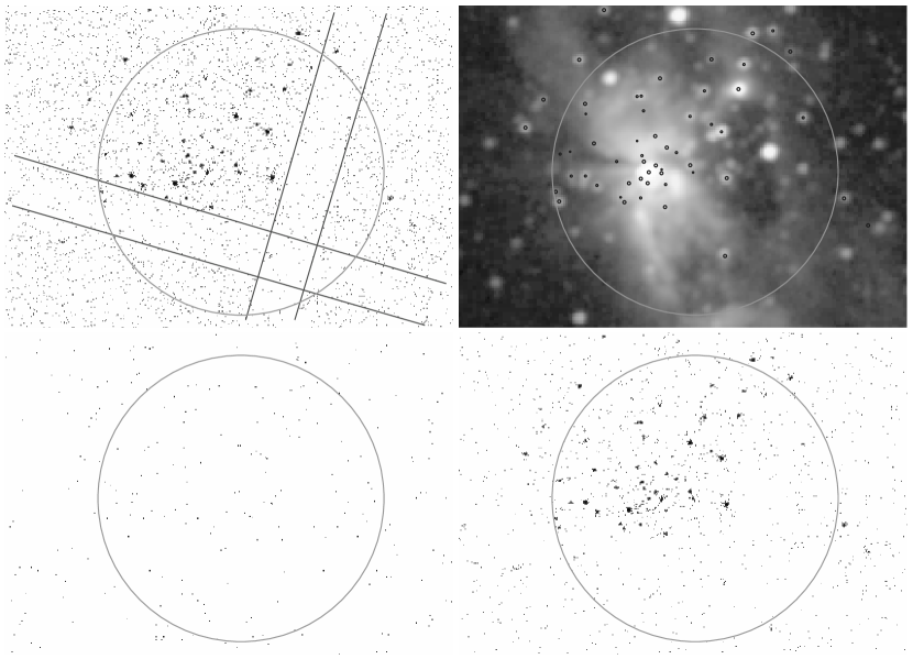
Figure 1: The field centered on S106 in the ACIS-I camera for the full energy range of the detectors (top left), in the 2MASS $K$-band (top right), in the ACIS-I camera for the energy range $\Delta E=0.2-1.0$ keV (bottom left) and in the ACIS-I camera for the energy range $\Delta E=1.0-7.5$ keV (bottom right). The X-ray sources detected in the Chandra image have been overlaid on the 2MASS image and are represented by small circles. The core size of S106 is shown as a large circle (radius 1.1. arcmin). In the top left image the lines indicate the position of the CCD gaps in the ACIS camera.

Fig. 1 shows the field centered on S106 as seen in the ACIS-I camera (for various energy ranges) and in the $K$-band of the 2MASS survey. Only the area within 1.1 arcmin from the centre is displayed for clarity, although we applied our analysis to an area within 4.4 arcmin from the cluster centre. A radius of 4.4 arcmin was chosen with the aim of studying the cluster with a minimal contamination from foreground and background sources in the absence of a membership list. The chosen radius corresponds to 4 times the S106 core radius as estimated by LDK02 and therefore should contain the large majority of the cluster members. At the same time, it does not extends to regions too far off-axis, where the sensitivity to X-ray sources would be lower (because of vignetting and because the Chandra PSF widens).

A clustering of X-ray sources is visible in the ACIS-I image obtained for the entire energy range ($\Delta E=0.2-10.0$ keV), although the cluster is ’cut’ by the ACIS CCD gaps, which determine a reduced sensitivity region. The 2MASS $K$-band image is dominated by the young massive stellar object S106 IRS4 (a bright IR source) near the center and by the double-lobed infrared nebula around it. S102 IRS4 is thought to be the engine which powers the double-lobed nebula and the associated H ii region (Gehrz et al., 1982). The X-ray sources detected with Pwdetect are overlaid on the 2MASS image.

As discussed below, most X-ray sources (and in particular S106 IRS 4) have an IR counterpart. A number of X-ray sources close to S106 IRS 4 have no counterpart unresolved from S106 IRS 4 in the 2MASS image, while north of S106 IRS 4 an example of a double X-ray source with an unresolved IR counterpart can be seen. The cluster center coordinates as given by LDK02 (the center of the big circle in Fig. 1) lies 0.3 arcmin off-axis in the Chandra observation.

In Fig. 1 the ACIS-I images of the field centered on S106 for a soft ($\Delta E=0.2-1.0$ keV) and a hard energy band ($\Delta E=1.0-7.5$ keV) are also shown. The great majority of the X-ray sources in the direction of S106 are not visible for energies lower the 1.0 keV, while are clearly visible in the hard band, as expected on the basis of the high extinction toward the cluster (see below).

In Table 1 we list the coordinates for all the X-ray sources detected with Pwdetect within a radius of 4.4 arcmin from the center of S106. A total of 87 X-ray sources are detected, of which 45 are within the S106 core radius. The X-ray source density within the 4.4 arcmin radius is 1.4 arcmin^-2, 10 times higher than in the rest of the ACIS-I field. The X-ray source density within the 1.1 arcmin core radius is 11.8 arcmin^-2. Most of the detected sources are rather weak, with a count rate below 1 ct ks^-1. The faintest source is source 9 with a count rate of 0.16 ks^-1, which corresponds to a flux of $1.6\times 10^{-15}$ erg cm^-2 s^-1and an intrinsic (unabsorbed) flux of $4.2\times 10^{-15}$ erg cm^-2 s^-1. Only 7 sources (sources 22, 30, 32 39, 60, 68 and 72) have a count rate just above 2 ct ks^-1.

For the sources with an IR counterpart the values of their magnitude in the $J$, $H$ and $K$ bands are also given in Table 1 together with the radial distance from the possible IR counterpart. An X-ray source was considered to have a possible IR counterpart if an IR source is present in the 2MASS PSC catalogue within a radius of 3 arcsec from the X-ray position. Of the 87 sources within the 4.4 arcmin radius 64 have a possible IR counterpart. Source 82 has two possible IR counterparts, while sources 55 and 58 have the same IR counterpart. All the 7 brightest X-ray sources have an IR counterpart.

The X-ray counterpart of S106 IRS 4 is source 50 in our list. It is a weak source with a count rate of $0.3\pm 0.11$ ct ks^-1; its X-ray position is less than 0.5 arcsec away from the coordinates of S106 IRS 4 in the 2MASS PSC, which agrees well with the coordinate for S106 IRS 4 given in Schneider et al. (2002) ($\alpha,\delta$= 20:27:26.74, 37:22:48), but are more than 12 arcsec away from the position given for this object in the Simbad database, which corresponds to the coordinates given in Gehrz et al. (1982).

To quantify the visual impression that the great majority of the X-ray sources detected in the direction of S106 have hard spectra, (and thus are not visible below 1.0 keV) we have run Pwdetect also on the energy-filtered ACIS-I event lists. Only 8 sources (flagged with a ’s’ in Table 1) are detected by the algorithm in the soft energy band ($\Delta E=0.2-1.0$ keV) within a radius of 4.4 arcmin from the center of S106. All of these 8 sources have an IR counterpart, and only one is within the S106 core radius. In the total ACIS-I field 27 out 125 sources are detected in the soft band, implying that, within 4.4 arcmin from the center of S106, the fraction of soft sources (9%) is more than 6 times lower then in the rest of the ACIS-I field (60%).

LDK02 derive, for the stars belonging to S106, extinction coefficients in the $K$ band ranging from $A_{K}=0.5$ to $A_{K}=4.0$. Given the conversion factor (Rieke & Lebofsky, 1985):

$$A_{K}=0.11A_{V}$$ (1)

and the relation (see e.g. Cox, 2000):

$$\mbox{$N({\rm H})$}/A_{V}=1.9\times 10^{21}$ \leavevmode\nobreak\ cm$^{-2}$\leavevmode\nobreak\ mag$^{-1}$$ (2)

the absorbing column density for members of S106 must be $\mbox{$N({\rm H})$}\ga 8.5\times 10^{21}$  cm^-2. The fact that the majority of the sources are not visible in the ACIS camera for energies below 1.0 keV is consistent with such high absorbing column densities. Indeed, if we assume as a typical spectrum for the sources listed in Table 1 an absorbed Raymond-Smith plasma model with $\mbox{$N({\rm H})$}=2.0\times 10^{21}$  cm^-2, plasma temperature $kT=1.5$ keV and metal abundance $Z=0.2\,Z_{\sun}$ then, using the pimms simulator at Heasarc, the expected ratio of the count rate between the soft and the total band is 0.15. This estimate is not very sensitive to the assumed X-ray temperature in the range 1$-$ 3 keV.

Table 1: X-ray sources detected in the Chandra data within 4.4 arcmin from the center of S106. For those sources for which an IR counterpart in the 2MASS PSC exists the $J,H,K$ magnitude are given together with the separation ($r$) from the possible counterparts. The ’s’ flag indicates sources which are also detected in the soft band ($\Delta E=0.2-1.0$ keV). The value of $\log L_{X}$ derived from Eq. 3 for the sources with IR counterpart is also given. Seven sources are inconsistent with the estimated age and distance of S106, therefore, their luminosity cannot be computed using Eq. 3. We have marked these sources with ’f’.

Source	RA(J2000)	Dec(J2000)	Count rate	$J$	$H$	$K$	$r$	$\log L_{X}$	Soft
			(ks)-1				(arcsec)	($\log\leavevmode\nobreak\$erg s-1)
1	20:27:06.1	37:23:29	0.59 $\pm$ 0.18	14.5	13.3	13.0	0.68	29.6
2	20:27:07.4	37:21:11	0.40 $\pm$ 0.14	14.4	13.2	12.7	0.63	29.7
3	20:27:08.5	37:25:06	0.35 $\pm$ 0.12	14.9	13.3	12.5	1.05	29.9
4	20:27:09.0	37:22:18	0.37 $\pm$ 0.13	12.9	12.0	11.6	2.29	29.4
5	20:27:09.2	37:23:31	0.17 $\pm$ 0.09	13.3	12.3	11.9	0.40	29.2
6	20:27:09.2	37:24:32	0.55 $\pm$ 0.17	16.3	15.1	14.5	0.76	29.7
7	20:27:09.6	37:21:38	0.25 $\pm$ 0.18	13.6	12.6	12.2	0.97	29.3
8	20:27:09.9	37:22:28	0.57 $\pm$ 0.18	16.1	14.4	13.4	0.44	30.1
9	20:27:10.7	37:24:42	0.16 $\pm$ 0.07	15.8	14.5	13.9	0.28	29.2
10	20:27:12.1	37:23:60	0.44 $\pm$ 0.15	15.0	13.1	12.0	0.28	30.2
11	20:27:12.2	37:22:53	0.18 $\pm$ 0.08	15.5	14.1	13.6	0.54	29.3
12	20:27:12.5	37:25:02	0.48 $\pm$ 0.16	16.1	14.5	13.9	0.63	29.9
13	20:27:13.1	37:22:07	0.16 $\pm$ 0.08	17.2	15.2	14.4	0.45	29.6
14	20:27:13.3	37:22:13	0.49 $\pm$ 0.15	-	-	-	-	-
15	20:27:14.9	37:22:43	0.21 $\pm$ 0.08	16.0	14.2	13.6	0.35	29.6
16	20:27:16.4	37:22:02	0.28 $\pm$ 0.12	15.5	14.8	14.6	0.47	f
17	20:27:18.0	37:24:39	1.29 $\pm$ 0.19	16.0	14.0	13.2	0.42	30.6
18	20:27:18.3	37:22:23	0.34 $\pm$ 0.14	-	-	-	-	-
19	20:27:18.4	37:21:04	0.20 $\pm$ 0.09	-	-	-	-	-
20	20:27:19.2	37:22:36	0.72 $\pm$ 0.21	15.0	13.5	12.9	0.65	30.1
21	20:27:20.8	37:23:13	0.23 $\pm$ 0.11	15.1	13.3	12.4	0.37	29.8
22	20:27:21.3	37:23:43	3.53 $\pm$ 0.46	17.4	15.1	13.8	0.18	31.1
23	20:27:21.4	37:24:28	0.23 $\pm$ 0.09	16.8	14.9	13.7	0.64	29.8
24	20:27:22.0	37:23:53	0.18 $\pm$ 0.08	16.0	13.8	12.5	0.25	29.8
25	20:27:22.5	37:19:50	0.78 $\pm$ 0.15	-	-	-	-	-
26	20:27:22.8	37:23:52	1.48 $\pm$ 0.20	13.4	12.1	11.6	0.22	30.3
27	20:27:22.8	37:24:14	1.05 $\pm$ 0.17	14.2	13.6	13.3	0.09	f	s
28	20:27:23.1	37:23:38	0.29 $\pm$ 0.11	13.8	12.2	11.1	0.15	29.9
29	20:27:23.3	37:23:26	0.83 $\pm$ 0.16	13.8	11.1	9.0	0.45	30.8
30	20:27:23.8	37:22:45	2.12 $\pm$ 0.23	13.3	11.9	11.6	0.28	30.5	s
31	20:27:23.8	37:22:09	0.70 $\pm$ 0.31	14.1	12.8	11.9	1.22	30.2
32	20:27:24.0	37:23:07	2.31 $\pm$ 0.24	11.3	10.6	10.2	0.23	30.2
33	20:27:24.4	37:23:10	0.49 $\pm$ 0.16	15.2	13.5	11.5	0.38	30.3
34	20:27:24.4	37:23:40	0.32 $\pm$ 0.12	15.4	14.0	13.6	0.22	29.5
35	20:27:24.6	37:18:29	0.67 $\pm$ 0.19	13.4	13.0	12.9	0.37	f	s
36	20:27:24.6	37:23:25	0.32 $\pm$ 0.12	14.0	12.5	12.0	0.08	29.7
37	20:27:25.1	37:22:48	0.32 $\pm$ 0.13	-	-	-	-	-
38	20:27:25.2	37:22:51	0.65 $\pm$ 0.19	14.0	13.0	12.9	0.28	28.8
39	20:27:25.2	37:23:14	2.18 $\pm$ 0.24	14.3	12.3	11.2	0.10	30.9
40	20:27:25.7	37:22:57	0.40 $\pm$ 0.13	-	-	-	-	-
41	20:27:26.1	37:22:59	0.41 $\pm$ 0.13	13.0	12.0	11.0	2.06	29.9
42	20:27:26.1	37:22:42	0.17 $\pm$ 0.08	-	-	-	-	-
43	20:27:26.2	37:22:32	0.56 $\pm$ 0.17	13.5	11.1	10.3	0.74	30.4
44	20:27:26.3	37:22:49	0.19 $\pm$ 0.11	-	-	-	-	-
45	20:27:26.3	37:22:47	0.76 $\pm$ 0.21	-	-	-	-	-
46	20:27:26.3	37:23:31	0.26 $\pm$ 0.10	15.1	13.2	12.2	0.61	29.9
47	20:27:26.5	37:24:30	0.41 $\pm$ 0.13	15.7	14.1	13.6	0.57	29.8
48	20:27:26.5	37:22:51	0.34 $\pm$ 0.12	-	-	-	-	-
49	20:27:26.5	37:23:05	0.36 $\pm$ 0.14	12.3	10.8	11.0	1.19	29.5
50	20:27:26.8	37:22:48	0.30 $\pm$ 0.11	10.4	7.7	5.9	0.44	30.3

Table 1: (continued) X-ray sources within 4.4 arcmin of S106 center.

Source	RA(J2000)	Dec(J2000)	Count rate	$J$	$H$	$K$	$r$	$\log L_{X}$	Soft
			(ks)-1				(arcsec)	($\log\leavevmode\nobreak\$erg s-1)
51	20:27:26.8	37:22:43	0.30 $\pm$ 0.11	-	-	-	-	-
52	20:27:27.0	37:22:53	0.23 $\pm$ 0.09	-	-	-	-	-
53	20:27:27.0	37:23:16	0.27 $\pm$ 0.11	-	-	-	-	-
54	20:27:27.1	37:22:55	0.98 $\pm$ 0.16	12.2	11.9	10.5	2.08	30.2
55	20:27:27.1	37:23:23	0.43 $\pm$ 0.14	13.9	12.3	11.6	0.49	30.0
56	20:27:27.1	37:22:45	0.19 $\pm$ 0.08	-	-	-	-	-
57	20:27:27.1	37:22:36	0.53 $\pm$ 0.16	-	-	-	-	-
58	20:27:27.2	37:23:23	0.39 $\pm$ 0.13	13.9	12.3	11.6	1.54	29.9
59	20:27:27.2	37:23:02	0.26 $\pm$ 0.11	13.5	11.0	9.8	2.18	30.1
60	20:27:27.6	37:22:43	2.45 $\pm$ 0.25	14.0	12.6	10.8	3.02	31.0
61	20:27:27.7	37:22:34	0.35 $\pm$ 0.13	-	-	-	-	-
62	20:27:27.9	37:22:36	0.42 $\pm$ 0.14	14.6	13.1	9.5	2.12	30.5
63	20:27:28.0	37:21:29	0.21 $\pm$ 0.08	-	-	-	-	-
64	20:27:28.0	37:22:53	0.43 $\pm$ 0.15	-	-	-	-	-
65	20:27:28.2	37:24:47	0.96 $\pm$ 0.15	16.4	14.6	13.7	0.16	30.3
66	20:27:28.5	37:24:03	0.28 $\pm$ 0.10	14.8	13.2	12.6	0.35	29.7
67	20:27:28.8	37:19:50	0.68 $\pm$ 0.20	13.4	12.8	12.6	0.21	f	s
68	20:27:28.8	37:19:45	3.71 $\pm$ 0.30	13.7	13.2	12.8	0.39	f	s
69	20:27:28.8	37:22:42	0.44 $\pm$ 0.15	15.0	13.4	12.8	0.71	29.9
70	20:27:28.9	37:23:01	0.62 $\pm$ 0.11	-	-	-	-	-
71	20:27:29.2	37:23:15	0.27 $\pm$ 0.10	-	-	-	-	-
72	20:27:29.2	37:22:46	2.48 $\pm$ 0.25	14.7	12.9	12.1	0.10	30.8
73	20:27:29.3	37:23:19	0.20 $\pm$ 0.08	15.4	13.9	12.6	0.50	29.8
74	20:27:29.5	37:23:40	0.98 $\pm$ 0.16	14.9	13.1	12.2	0.25	30.4
75	20:27:29.8	37:22:46	0.28 $\pm$ 0.10	15.6	13.9	13.0	0.29	29.8
76	20:27:29.8	37:22:57	0.17 $\pm$ 0.09	-	-	-	-	-
77	20:27:30.2	37:22:56	0.30 $\pm$ 0.11	-	-	-	-	-
78	20:27:30.3	37:22:34	0.71 $\pm$ 0.25	14.8	13.1	12.2	0.31	30.3
79	20:27:30.4	37:22:39	0.34 $\pm$ 0.14	15.5	13.9	13.5	0.21	29.6
80	20:27:30.7	37:24:29	0.31 $\pm$ 0.11	12.9	12.4	12.2	0.22	f	s
81	20:27:30.8	37:24:11	0.18 $\pm$ 0.08	16.3	14.3	13.2	0.57	29.8
82-a	20:27:30.9	37:23:21	0.34 $\pm$ 0.12	15.5	14.0	14.3	0.21	29.6
82-b	idem	idem	idem	15.6	14.0	13.7	2.63	28.5
83	20:27:31.6	37:23:08	0.67 $\pm$ 0.13	14.5	12.9	12.2	0.17	30.2
84	20:27:35.5	37:20:24	0.36 $\pm$ 0.13	11.7	11.2	11.1	2.58	f	s
85	20:27:40.5	37:21:47	0.27 $\pm$ 0.11	16.2	15.1	14.6	0.41	29.2
86	20:27:41.6	37:25:35	0.29 $\pm$ 0.12	-	-	-	-	-
87	20:27:42.7	37:23:40	1.06 $\pm$ 0.17	14.0	13.2	12.8	0.46	29.2	s

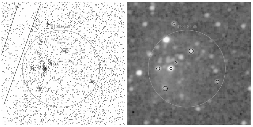
Figure 2: The field centered on S106 south in the ACIS-I camera (left) and in the 2MASS $K$-band image (right). The X-ray sources detected in the Chandra image have been overlaid on the 2MASS image and are represented by small circles with size proportional to the X-ray count rate. The selection area that we have used for S106 south is shown as a large circle (radius 0.8 arcmin). In the ACIS image the lines indicate the position of the CCD gaps.

2.1 S106 south

As mentioned in the Introduction, Schneider et al. (2002) identify the cluster S106 as a primary star formation site coincident with the prominent peak in CO emission. They also detect a second weaker CO peak located 5 arcmin south of S106 IRS 4 which harbors a small IR cluster and nebulosity and refer to it as “S106 south”.

Fig. 2 shows the field centered around S106 south in the ACIS-camera and in the 2MASS $K$ band. An increase in source density in the direction of S106 south is visible in the Chandra image. The approximate center of this group of X-ray sources is at $\alpha,\delta=$ 20:27:23.2, 37:17:33 (5 arcmin off-axis in the Chandra data). In Table 2 the coordinates and 2MASS IR photometry for all X-ray sources within a radius of $0.8$ arcmin from this position are listed. A total of 6 sources have been detected, making the source density within this area 20 times higher than in the rest of the field (excluding the area of $4.4$ arcmin radius from the center of S106).

All of the 6 sources have an IR counterpart within a radial distance of $3$ arcsec, and only one of them is visible in the soft band.

Table 2: X-ray sources detected in the Chandra data using Pwdetect within 0.8 arcmin from the center of S106 south. For those sources for which an IR counterpart in the 2MASS PSC exists the $J,H,K$ magnitude are given. The ’s’ flag indicates sources which are also detected in the soft band ($\Delta E=0.2-1.0$ keV). The value of $\log L_{X}$ derived from Eq. 3 is also given.

Source	RA(J2000)	Dec(J2000)	Count rate	$J$	$H$	$K$	$r$	$\log L_{X}$	Soft
			(ks)-1				(arcsec)	($\log\leavevmode\nobreak\$erg s-1)
1	20:27:20.0	37:17:16	0.51 $\pm$ 0.17	14.6	13.5	13.1	0.57	29.5
2	20:27:22.8	37:17:55	0.64 $\pm$ 0.19	15.2	13.2	11.6	0.27	30.4
3	20:27:24.4	37:17:41	0.38 $\pm$ 0.15	15.8	14.1	13.6	0.79	29.8
4	20:27:24.8	37:17:33	1.28 $\pm$ 0.20	11.0	10.2	9.8	0.58	30.1
5	20:27:25.4	37:17:08	0.82 $\pm$ 0.23	16.5	14.3	12.6	1.71	30.6	s
6	20:27:26.2	37:17:33	0.50 $\pm$ 0.17	14.8	12.7	11.4	0.44	30.3

3 Results

3.1 Color-magnitude and color-color diagrams for the IR counterparts to X-ray sources

To compare the population of the X-ray sources detected in the Chandra exposure with the population of S106 as defined by LDK02 we have constructed a $K$ vs. $J-K$ color magnitude diagram (Fig. 3) for the X-ray sources listed in Tables 1 and 2 which have an IR counterpart in the 2MASS PSC.

In the diagram 2 Myr isochrones are shown for 4 values of extinction ($A_{K}={\rm 0,1,2,3}$). Reddening vectors have been computed following the same relation adopted by LDK02, $A_{K}=R_{K}\times E(J-K)$ where $E(J-K)$ is the colour excess ($E(J-K)=(J-K)-(J-K)_{0}$) and $R_{K}=0.66$ (Rieke & Lebofsky, 1985). The isochrones are from Siess et al. (2000), for a metal abundance $Z=0.02$ plus overshooting, shifted to the estimated distance of S106 (600 pc). Various simplifying assumptions apply to these models, e.g. they include neither rotation nor accretion, and we caution that evolutionary models for pre-main sequence stars are not yet well established. Stassun et al. (2004) recently reported the discovery of a double-lined, spectroscopic, eclipsing binary in the Orion star-forming region, with measured masses of 1.01 M_☉ for the primary and 0.73 M_☉ for the secondary. They used their measurements of the fundamental stellar properties for both components to test the predictions of pre-main sequence stellar evolutionary tracks. None of the models they examined (including the one by Siess et al., 2000) correctly predicts the masses of the two components simultaneously.

In Fig. 3 seven sources have been highlighted using a triangle (sources 16, 27, 35, 67, 68, 80 and 84). These sources fall on the blue side of the 2 Myr isochrone for zero extinction and therefore are inconsistent with the estimated age and distance of S106. There is evidence that these maybe foreground sources. They do not meet the membership criteria used by LDK02 (their extinction coefficient being too low) and all of them but source 16 are detected in the Chandra soft band, consistent with their being less absorbed than the others. Note, however, that sources 30 and 87, that have been flagged as “soft”, are not inconsistent with a 2 Myr isochrone and the value of their extinction coefficient as computed by LDK02 is consistent with their membership criteria.

The sources in our sample appear very scattered in the color-magnitude diagram, implying highly variable absorption. LDK02 find the same large scatter for their IR sample of sources belonging to S106 (according to their selection criteria), and suggest that, while this scatter is partly due to large and variable absorption, it is probably also an effect of the unreliability of the 2MASS photometric data in this very crowded area. From the color-magnitude diagram it appears that the X-ray selected sample contains a number of heavily absorbed massive stars. The brightest of all, with $K=5.9$, is the massive young stellar object S106 IRS 4 at the center of the S106 complex.

The color-magnitude diagram also provides an indication of the completeness limit of our X-ray survey, which is at around $K\simeq 12$, as we have verified by plotting differential star counts versus apparent magnitude. For a 2 Myr isochrone $K=12$ corresponds to stars of mass $M\simeq 0.5\,M_{\sun}$ for low extinction ($A_{K}<0.1$) and $M\ga 1.2\,M_{\sun}$ for extinction coefficients $A_{K}\geq 1.0$

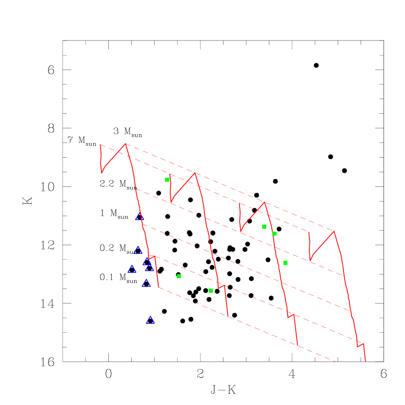
Figure 3: Color magnitude diagram for the IR counterparts to the X-ray sources detected within 4.4 arcmin from the center of S106 (black circles) and within S106 south (gray squares). Theoretical 2 Myr isochrones are also shown for different extinction coefficients (from left to right $A_{K}={\rm 0,1,2,3}$). The dashed lines indicate the reddening vector for stars of constant mass. Points with a triangle indicate sources inconsistent with the theoretical 2 Myr isochrone (see text for details).

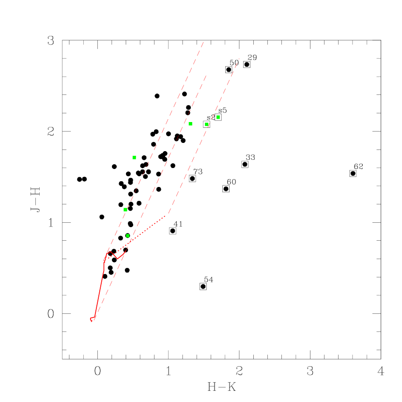
Figure 4: Color-color diagram for the IR counterparts to the X-ray sources detected within 4.4 arcmin from the center of S106 (circular black points) and within S106 south (square gray points). The solid line at lower-left is the theoretical 2 Myr isochrone. The dotted line yields the locus of dereddened colours of classical T Tauri stars according to Meyer et al. (1997). The dashed lines mark the reddening bands. The most heavily reddened stars are identified.

The $J-H$ versus $H-K$ color-color diagram in Fig. 4 allows normally reddened stars to be discriminated from star with IR excess (indicative of warm circumstellar dust in addition to a reddened photosphere). The intrinsic colours for stars on a 2 Myr isochrone are indicated by the solid line, whereas the dotted line yields the locus of dereddened colours of classical T Tauri stars according to Meyer et al. (1997). The dashed lines define the region of normal reddening using the reddening law from Rieke & Lebofsky (1985) (the normal reddening region of main sequence stars would be very similar to the one of the stars on the 2 Myr isochrone). The scatter of the X-ray sources outside this region is significant and it is probably an effect of the unreliability of the 2MASS photometric data in this crowded area. Nevertheless in the diagram we have identified 10 sources which appear to have significant IR excess (i.e. lie to the right of the normal reddening region) and therefore could be embedded young objects. The presence of an IR excess for source 50 (S106 IRS 4) is already known from the literature (Felli et al., 1984; Gehrz et al., 1982; Hodapp & Rayner, 1991).

In the color-magnitude diagram sources 29, 50 (S106 IRS 4) and 62 appear to be massive objects (with masses above $7\,M_{\sun}$). This estimate does not take into account the presence of an IR excess which may lead to overestimate the star mass. This is not the case however for S106 IRS 4, for which estimates in the literature independently indicate a mass greater than $15\,M_{\sun}$ (Felli et al., 1984).

3.2 X-ray luminosity as a function of stellar mass

To convert detector count rates to intrinsic X-ray luminosity we have derived, using the pimms software at Heasarc, a conversion factor between (unabsorbed) source flux and observed count rate, taking into account the absorption. The absorbing column density for each star was derived by first estimating $A_{K}$ and then deriving $N({\rm H})$ using Eqs. (1) and (2). The value of $A_{K}$ was determined assuming that all sources in S106 and S106 south would intrinsically lie on the theoretical 2 Myr isochrone and then measuring the displacement along the reddening vector. No extinction can obviously be derived for sources 16, 27, 35, 67, 68, 80 and 84, which lie on the blue side of the isochrone.

Because of the shape of the 2 Myr isochrone a degeneracy is present for mass ranges 2.2–7.0 $M_{\sun}$ and 0.2–0.3 $M_{\sun}$; lacking additional information (e.g. spectral types or optical magnitudes) this degeneracy cannot be resolved. We thus, somewhat arbitrarily, decided to associate the mass derived through the rightmost intersection with the isochrone for the mass range 2.2–7.0 $M_{\sun}$, and redefined the isochrone for the mass range 0.2–0.3 $M_{\sun}$ using a tangent along the reddening vector at $M=0.2\,M_{\sun}$ (shown in Fig. 3 as a thin line).

As a typical X-ray spectrum for our sample we assumed a one-temperature plasma model with $kT=2.16$ keV and a coronal metal abundance $Z=0.2Z_{\sun}$, deriving, for $\mbox{$N({\rm H})$}=1.0\times 10^{22}$ cm^-2 and a count rate of 1 ks^-1, a conversion factor of $F_{\rm X\leavevmode\nobreak\ intr}=2.7\times 10^{-14}$erg cm^-2 s^-1. The conversion factor scales almost linearly with $N({\rm H})$ (for $\mbox{$N({\rm H})$}=[0.5-6.0]\times 10^{22}$ cm^-2, the range in which all our objects fall, see below), so that

$$F_{\rm X\leavevmode\nobreak\ intr}=2.7\times 10^{-14}\times\mbox{$N({\rm H})$}\ \times{\rm ct}\leavevmode\nobreak\ \leavevmode\nobreak\ \leavevmode\nobreak\ [{\rm erg\leavevmode\nobreak\ cm^{-2}\leavevmode\nobreak\ s^{-1}}]$$ (3)

where ${\rm ct}$ are the source counts in units of ks^-1 and $N({\rm H})$ is the absorbing column density in units of $10^{22}$ cm^-2. The error introduced in the flux estimate by the linear approximation is below 30%.

In all but three cases we derived a value of $A_{K}$ corresponding to an absorbing column density within the range $[0.5-6.0]\times 10^{22}$ cm^-2. For sources 38, 82-a and 87 we derived values of $A_{K}\leq 0.07$ (corresponding to $\mbox{$N({\rm H})$}<0.1\leavevmode\nobreak\ \times 10^{22}$ cm^-2), significantly below the absorbing column densities derived for all the other sources in our sample (which has a median of $A_{K}=1.1$); we have therefore excluded these sources from the rest of the analysis. Having determined for a star its intrinsic magnitude in $K$, as described above, an estimate of its mass is readily available by using the 2 Myr isochrone.

The derived X-ray luminosity as a function of the stellar mass is shown in Fig. 5; 61 sources are included in the final samples, i.e. all sources in Tables 1 and 2 with the exception of sources 16, 27, 35, 38, 67, 68, 80, 82-a, 84 and 87. The median X-ray luminosity for stars in different mass intervals is also shown, using the same mass bins adopted by Flaccomio et al. (2003) in their analysis of the X-ray activity indicators for members of the Orion Nebula Cluster (ONC). The median X-ray luminosities are summarised in Table 3. We note that for masses lower than $0.5\,M_{\odot}$ the derived median X-ray luminosities are systematically higher than the corresponding ONC stars while the reverse is true for $M>0.5\,M_{\odot}$. The values at lower masses ($M\leq 0.5\,M_{\odot}$), which corresponds to lower fluxes, are likely biased to higher X-ray luminosities due to lack of a parent sample of cluster members. In their analysis of the ONC Flaccomio et al. (2003) made use of an optical sample of cluster members in order to place upper limits on X-ray luminosities. Lacking such a sample for the S106 clusters we are not able to place upper limits. The fact that for $M>0.5\,M_{\odot}$ the values of median $L_{X}$ for our sample are systematically lower than for the ONC could be an indication of some physical difference between the S106 region and the ONC, such as a different fraction of binaries. Nevertheless the statistic is too small and the uncertainties too large to attach any significance to this difference.

A trend of increasing X-ray luminosities with star mass is clearly visible in Fig. 5. Two areas, one for 0.17–0.46 $M_{\sun}$ and one for 2.9–9.4 $M_{\sun}$, are devoid of points. This is, partly, an effect of the way we have chosen to circumvent the degeneracy in value of $A_{K}$ for some mass ranges (see above), partly, it is a feature of the data themselves. We note also that lacking optical/IR spectral studies of the members of the S106 clusters we do not know neither the spectral energy distribution nor the spectral characteristics of the stars in our sample and are therefore unable to classify them.

In Fig. 5 the star with a mass estimate of $102$ $M_{\sun}$ is source 50, corresponding to the central exciting star S106 IRS 4. The value of $102$ $M_{\sun}$ is very probably overestimated, due to the fact that the method we have used to derive a mass value for each star does not take into account the possible presence of an IR excess, which in this case is known to be present (e.g. Felli et al., 1984 and Fig. 4). Indeed, the masses of all stars in our sample for which we identified a significant IR excess maybe affected by such an error. For S106 IRS 4 the estimates in the literature indicate a mass greater than $15\,M_{\sun}$ (Felli et al., 1984) and therefore the presence of an IR excess does not affect the placement of S106 IRS 4 in the highest mass bin.

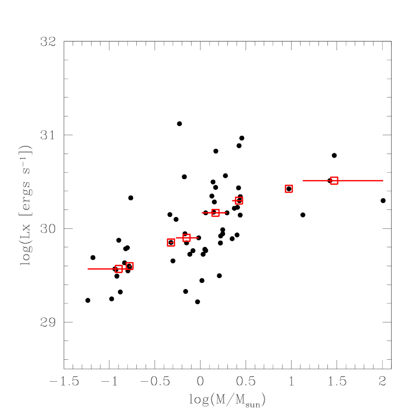
Figure 5: Scatter plot of intrinsic X-ray luminosities as a function of mass for the sample of 61 sources defined in the text. The gray horizontal lines indicate the median $L_{\rm X}$ for the corresponding mass interval. The abscissa of the empty-squares is the median mass for each subsample. The same mass intervals (in units of $M_{\sun}$) as in Flaccomio et al. (2003) have been considered: $(0,0.16]$, $(0.16,0.25]$, $(0.25,0.5]$, $(0.5,1.0]$, $(1.0,2.0]$, $(2.0,3.0]$, $(3.0,10]$ and $(10,\infty)$

.

Table 3: Median value of the X-ray luminosity (second column) for our sample of 61 sources in S106 and S106 south for different mass ranges. These values can be compared with the values for members of the ONC (fourth column), as derived by Flaccomio et al. (2003). The number of sources of our sample within each mass range is also given.

Mass	$\log(L_{\rm X})$	N. src.	$\log(L_{\rm X})$ ONC
$M_{\sun}$	log(erg s-1)		log(erg s-1)
$<0.16$	29.57	12	29.00
0.16–0.25	29.60	3	29.15
0.25–0.50	29.85	3	29.60
0.50–1.00	29.90	10	30.05
1.00–2.00	30.17	18	30.45
2.00–3.00	30.30	10	31.20
3.00–10.0	30.42	1	30.50
$>10.0$	30.51	4	30.90

3.3 Spectral and timing analysis of the brightest X-ray sources

A spectral and timing analysis was carried out for the seven brightest X-ray sources in the list of Table 1 (sources 22, 30, 32, 39, 60, 68, 72). Their light curves are shown in Fig. 6. Sources 22 and 68 present large-amplitude variability, and source 22 is not visible (no photons are detected) for the first 10 ks of the Chandra exposure; the rise in the source luminosity at 10 ks is impulsive and it is followed by a decay lasting about 10 ks, with a behavior typical of stellar flares. The mass of source 22 is estimated at $M\simeq 0.6\,M_{\sun}$. The time variability of source 68 is remarkable, with the source counts suddenly increasing to more than 10 times the previous level in about 2 ks and then decreasing abruptly again to a level about 3 times higher than before the jump. We do not provide an estimate for the mass as its position in the color-magnitude diagram is inconsistent with a 2 Myr isochrone at 600 pc. Both in the X-ray image and in the 2MASS data source 68 has an apparent companion, source 67, at about $4.7$ arcsec. Both sources are visible in the X-ray soft band and their $A_{K}$ derived with the approach described by LDK02 are very similar, consistent with the two sources being physically associated.

The Kolmogorov-Smirnov (K-S) test, which measures the maximum deviation of the integral photon arrival times from a constant source model, was applied to the light curves, with the results summarised in Table 4. As expected sources 22 and 68 have a negligible probability of being constant. The probability of constancy is also low for sources 30 and 39.

The background subtracted spectra for the seven brightest sources are plotted in Fig. 6, together with the best-fit models. The ACIS-I spectra, rebinned to a minimum of 5 counts per energy bin, were fit with an absorbed one-temperature plasma model with metal abundance 0.2 of solar, a value typical for T Tauri stars (e.g. Favata et al., 2003). The best fit spectral parameters are summarised in Table 4. The average coronal temperature for all sources but source 68 (likely a foreground source) is $kT=3.1$ keV, excluding also source 30 because of the large uncertainty the average is $kT=2.4$ keV. From the spectral fits intrinsic X-ray luminosities have been derived (also shown in Table 4), assuming a source distance $d=600\leavevmode\nobreak\$pc.

Excluding source 68, the values of absorbing column densities derived for these sources are all higher than $5.0\times 10^{21}$ cm^-2 (corresponding to $A_{K}>0.3$), consistent with the sources being in a region of high extinction. Sources 30 and 32 have values of $N({\rm H})$ around the lower limit of the typical absorbing column density for our sample of 61 sources, so that they could also be active foreground stars. Nevertheless their $A_{K}$ is consistent with cluster membership, as is their X-ray luminosity.

The best-fit values of $N({\rm H})$ and $L_{\rm X}$ reported in Table 4 are consistent, within a factor of three for the X-ray luminosity and within $2\sigma$ for $N({\rm H})$, with the ones computed using the photometrically derived $N({\rm H})$ and assuming a typical spectrum. This provides a consistency check on the method used to derive $N({\rm H})$ and $L_{\rm X}$ for all other sources in our sample of 61 for which a spectral analysis was not possible.

Figure 6: ACIS-I light curves (left) and spectra (right) for the seven X-ray sources detected within a 4.4 arcmin radius from the center of S106, which are bright enough (count rate greater than 2 counts/ks) for a timing and spectral analysis to be carried out. The fits to the spectra with absorbed one-temperature plasma model are also shown.

Figure 6: continued – light curves (left) and spectra (right) for the seven brightest X-ray sources in S106.

Table 4: Summary of the derived X-ray properties for the 7 brightest sources in our sample. $N({\rm H})$ phot. gives the absorbing column density as derived from the IR photometric data (see Sect. 3.2 for the procedure). $N({\rm H})$and $kT$ give the best fit values for the absorbing column density and the plasma temperature as derived from spectral fitting of the ACIS-I data with one-temperature plasma models. The models’ reduced $\chi^{2}$ and null hypothesis probability are given in the two next columns. $F_{\rm x}$ and “$F_{\rm x}$ unabs.” give the observed and unabsorbed X-ray flux for the best fit model. $L_{\rm X}^{1}$ and $L_{\rm X}^{2}$ are, respectively, the luminosity derived from “$F_{\rm x}$ unabs” and the luminosity derived with the same approach as for all the other sources in our sample for which a spectral analysis was not possible. $M$ gives the stars’ estimated mass, and K-S indicates the probability of constancy according to the Kolmogorov-Smirnov statistical test. Unless otherwise specified, fluxes are in the energy range 0.8–7.5 keV. $N({\rm H})$ is in units of $N_{22}=10^{22}$ cm^-2, fluxes are in unit of $F_{-13}=10^{-13}\leavevmode\nobreak\$erg cm^-2 s^-1 and $L_{\rm X}$ in unit of $L_{30}=10^{30}$erg s^-1.

Source	$N({\rm H})$ phot.	$N({\rm H})$	$kT$	$\chi^{2}$	$P$	$F_{\rm x}$	$F_{\rm x}$ unabs.	$M$	$L_{\rm X}^{1}$	$L_{\rm X}^{2}$	K-S
	$N_{22}$	$N_{22}$	keV			$F_{-13}$	$F_{-13}$	$M_{\sun}$	$L_{30}$	$L_{30}$
22	3.3	9.7$\pm$5.5	2.64$\pm$2.46	0.62	0.79	0.7a	2.6a	0.6	11	13	0.25$\times 10^{-7}$
30	1.3	0.8$\pm$0.4	6.71$\pm$5.57	1.00	0.46	0.3	0.3	1.4	1.3	3.1	0.20$\times 10^{-2}$
32	0.6	0.9$\pm$0.4	2.61$\pm$1.02	0.66	0.87	0.3	0.4	2.4	1.7	1.6	0.22
39	3.1	4.1$\pm$1.0	1.23$\pm$0.37	1.20	0.25	0.3	2.0	2.7	8.6	7.6	0.56$\times 10^{-2}$
60	3.3	3.2$\pm$0.8	2.33$\pm$0.75	0.72	0.82	0.4	1.0	2.9	4.3	9.2	0.83$\times 10^{-1}$
68b	-	0.2$\pm$0.1	1.02$\pm$0.11	1.14	0.19	0.2	0.3	-	0.4	-	0.59$\times 10^{-7}$
72	2.4	2.1$\pm$0.6	2.99$\pm$1.27	0.79	0.73	0.4	0.8	1.5	3.5	6.7	0.18

^a range 1.4–7.5 keV
^b likely a foreground source: it is inconsistent with a 2 Myr isochrone at 600 pc

4 Discussion

4.1 S106 membership

In the Chandra image of the S106 star-forming region 87 X-ray sources were detected within a 4.4 arcmin radius of the center of the S106 cluster and 6 sources were detected within 0.8 arcmin radius of the S106 south cluster. Of these, 71 sources appear to have an IR counterpart in the 2MASS PSC catalogue and 22 have no IR counterpart within 3 arcsec from the X-ray position.

The 22 sources without IR counterpart are likely stars, members of the S106 cluster. At a flux level of the order of 10^-14 erg cm^-2 s^-1 the expected number density of background sources determined on the basis of the $\log N-\log S$ relationship for X-ray sources (see e.g. Hasinger et al., 2001) is 100–200 sources per square degree. The area of a circle with 4.4 arcmin radius is 0.017 square degree, so that the expected number of serendipitous extra-galactic sources for a low absorption field is between 2 and 3. In practice given the high absorption value in this field it is unlikely that any of these 22 sources is a background source (of galactic or extra-galactic origin). The fact that none of these 22 sources shows up in the soft X-ray band is an other indication that most of them are affected by significant absorbing column density and therefore are unlikely to be foreground sources.

From the sample of 71 X-ray sources with IR counterpart we selected a subsample of 61 sources which have (photometrically derived) high extinction levels ($N({\rm H})$ within a range of $[0.5-6.0]\times 10^{22}$ cm^-2) consistent with the sources being members of the clusters. Of all these 61 sources only two (source 30 and source S106 south number 4) are visible in the X-ray soft band. This is another, independent, indication of high column densities in front of most the sources in the final sample. Of the two sources that were detected in the soft band we were able to study source 30 in more detail, finding that it has the characteristics of a pre-main sequence star (PMS) in the outer edge of the association. Thus, the 61 members of the final sample are all likely members of the S106 star forming region.

4.2 Age of the association

For the final sample of 61 sources we studied the X-ray luminosity as a function of mass. As apparent from Fig. 5 and Table 3 there is a clear correlation between X-ray luminosities and star masses. The presence of a correlation between X-ray luminosity and star masses has been established for other star forming regions (e.g. Preibisch & Zinnecker, 2002 for IC 348, Flaccomio et al., 2003 for the ONC) and it is a consequence of the fact that members of star-forming regions are young and emit at similar, close-to-saturated levels of X-ray luminosity. The presence of such a correlation in our sample therefore indicates that the stars are young and physically associated. A sample of field stars at random distances would not present such a correlation.

For stars in the mass bins 0.5–2.0 $M_{\sun}$ we derive a median value of $L_{\rm X}=8\times 10^{29}\leavevmode\nobreak\$erg s^-1. Considering the age evolution of the X-ray luminosity of solar-mass stars, and using the values tabulated by Micela (2002) for the median $L_{\rm X}$ of a number of star forming regions, open clusters and nearby field stars, one finds that a median value of $L_{\rm X}=8\times 10^{29}\leavevmode\nobreak\$erg s^-1 is very similar to the median luminosities in the ONC, the $\rho$ Oph star-forming region and the $\alpha$ Per cluster. This indicates for the S106 clusters an age lower than $3\times 10^{7}$ yr. In addition, the median X-ray luminosity values derived here for the S106 star-forming region are, for all mass bins apart one ($2.0-3.0\leavevmode\nobreak\ M_{\sun}$), within a factor of 3 of the values derived by Flaccomio et al. (2003) for the ONC, consistent with the age of S106 being similar to the one of the ONC, as well as with the age estimate of Hodapp & Rayner (1991) (1–2$\times 10^{6}$ yr).

We note that the median value $L_{\rm X}\simeq 10^{30}$ erg s^-1 for stars in our sample with masses of 0.5–2.0 $M_{\sun}$ is not strongly dependent on the use of a 2 Myr year theoretical isochrone to estimate extinction coefficients and masses. We have repeated the same procedure using a zero age main sequence by Siess et al. (2000) and the median luminosity derived for stars within this mass range is essentially unchanged. This is because for stars with masses of 0.5–2.0 $M_{\sun}$ in the 2 Myr hypothesis the difference in mass estimate using a zero age main sequence is only a factor $\sim 2$. The value of $L{\rm x}$ is affected by the age assumption via the extinction coefficient and this estimate is also not so sensitive to the use of a 2 million year isochrone or a zero age main sequence. In the first case we derive a median value of $A_{K}=1.1$ and in the second case $A_{K}=1.5$.

We caution however that in general the use of a zero age main sequence rather than the appropriate isochrone can lead to significant over-estimate of the cluster total mass. For instance in our case the use of a zero age main sequence leads to 22 stars in our sample having more than $3\,M_{\sun}$ while using a 2 Myr isochrone one only finds 5 stars. This may explain the significant difference in cluster mass estimates by Hodapp & Rayner (1991) who derive a total mass of $140\,M_{\sun}$ and LDK02 who derive 400–600 $M_{\sun}$. LDK02 used a linear fit to a zero age main sequence while Hodapp & Rayner (1991) adopted isochrones between 0.1–2.0 Myr.

4.3 S106 IRS 4

S106 IRS 4 is a massive stellar object of spectral type O7–B0 and luminosity of [0.4–$1]\times 10^{5}\leavevmode\nobreak\ L_{\sun}$ (Gehrz et al., 1982; Felli et al., 1984). The line-of-sight extinction is estimated at $A_{V}=20$–$30$ (Eiroa et al., 1979; Simon et al., 1983). From 2MASS photometric data we estimated for S106 IRS 4 an extinction coefficient $A_{K}=3.35$, corresponding to $A_{V}=30$. The infrared images are consistent with a model in which the recently formed massive stars excites the biconical nebula from within a large irregular disk of gas and dust which is the remnant of the stellar collapse process (Gehrz et al., 1982, Harvey et al., 1987). The near infrared flux from S106 IRS 4 is probably not photospheric but results from scattered and thermal radiation from the inner region of a circumstellar shell.

Radio observations show the existence of a compact shell of radio emission surrounding S106 IRS 4 (Simon et al., 1983; Kurtz et al., 1994). This is interpreted as emission from a flowing ionized envelope from a short-lifetime-phase of the pre-main sequence evolution of a massive star (Simon et al., 1983; Felli et al., 1984) – an evolutionary state with high mass loss which follows an earlier accretion phase.

The rate at which S106 IRS 4 is losing mass is atypically high for a star of this bolometric luminosity. At $\dot{M}\sim 1.6\times 10^{-6}\,M_{\sun}$ yr^-1, corresponding to $\dot{M}/L\simeq[1.6$–$8]\times 10^{-11}M_{\odot}\,L_{\odot}^{-1}$ yr^-1 (Felli et al., 1984), this is 1–2 orders of magnitude higher than most normal early type stars and comparable to the values measured in Wolf-Rayet stars. At the same time the terminal wind velocity of $v_{\infty}\sim 200$ km s^-1 is lower than typical values measured for equally luminous stars, for which $v_{\infty}\sim 1000$–$1500$ km s^-1 (Panagia & Macchetto, 1982). Radio observations suggests that this wind may be mainly equatorial (Hoare et al., 1994). Schneider et al. (2002) attribute the dynamics of the molecular gas in the S106 region to the impact of the ionized wind of S106 IRS 4, driving a shock into an inhomogeneous molecular cloud.

The Chandra observation provides the first detection of S106 IRS 4 in X-rays. We estimated for this source an X-ray luminosity of $2\times 10^{30}$erg s^-1 assuming a plasma temperature $kT=2.16$ keV, as for all the other sources in our sample. This luminosity corresponds to $L_{\rm X}/L_{\rm bol}\sim[0.5-1]\times 10^{-8}$, which is about one order of magnitude lower than typically observed for older massive stars (Sciortino et al., 1990), although there is a large scatter ($\pm 1$ dex) on the $L_{\rm X}/L_{\rm bol}$ relation for massive stars (e.g. Moffat et al., 2002). The assumed X-ray plasma temperature for S106 IRS 4 is however likely too high for an early type star. Chlebowski et al. (1989) have shown that typical plasma temperatures for wind related emission in O stars are around $kT=0.5$ keV, significantly lower than the value we have assumed. Given the high absorption toward the source, the choice of plasma temperature is rather critical for determining the X-ray luminosity. Assuming $kT=0.5$ keV one derives for

S106 IRS 4 an intrinsic X-ray luminosity of $L_{\rm X}=4.8\times 10^{31}$ erg s^-1, corresponding to a range $L_{\rm X}/L_{\rm bol}\sim[1.2$–$3]\times 10^{-7}$, at the lower end of the typical values for O stars (Sciortino et al., 1990). On the basis of the correlations determined by Sciortino et al. (1990) in their study of X-ray emission from O-stars an X-ray luminosity of $4.8\times 10^{31}$ erg s^-1 is a factor of 15 below the value typical for stars with comparable mass loss, but it is similar to the X-ray luminosities found in relation to the star wind momentum flux ($F_{\rm m}=\dot{M}v_{\infty}=2\times 10^{27}\leavevmode\nobreak\ {\rm g\leavevmode\nobreak\ cm\leavevmode\nobreak\ s^{-2}}$).

Kohno et al. (2002) have recently reported the detection of X-ray emission from four high-mass YSOs in Mon R2, deriving typical best fit plasma temperatures, absorption column densities and X-ray luminosities of $\sim 2$ keV, $\sim 5$–$10\times 10^{22}$ cm^-2 and $10^{30}$–$10^{31}$erg s^-1, that is X-ray luminosities similar to the one derived here for S106 IRS 4. The X-ray flux from the Mon R2 high mass YSOs appears to be highly variable with flare-like behavior; because of this and the high plasma temperatures Kohno et al. (2002) suggest that the X-ray activity of these massive YSOs may be magnetically driven, in a similar way to that seen in low mass PMS stars.

Unfortunately, for S106 IRS 4 no plasma temperature can be determined, which means that we cannot compare it with the values derived for the Mon R2 sources and that we have to base the estimate of its X-ray luminosity on an assumed plasma temperature. Nevertheless, assuming a plasma temperature typical for older massive stars, the X-ray luminosity of S106 IRS 4 is consistent to the values predicted for older stars on the basis of their wind momentum flux, which is the dominating factor in determining the X-ray luminosity of a massive star (as established by Sciortino et al., 1990 – Fig. 16a). This suggests that the activity in S106 IRS 4 maybe wind-driven, with no need to invoke the presence of magnetically confined plasma. In S106 IRS 4, we would thus be witnessing the onset of X-ray emission from the wind, at a stage in which the protostar is still deeply embedded in the circumstellar material.

4.4 Other interesting sources

Among the 7 sources for which we were able to study the X-ray spectra, sources 32, 39 and 60 are intermediate mass stars, with estimated masses of 2.4, 2.7 and $2.9\,M_{\sun}$, respectively. Were they main sequence they would correspond to A stars, which are, at most, weak X-ray sources ($L_{\rm X}\la 3\times 10^{27}$ erg s^-1, see e.g. Favata & Micela, 2003). Given their young age however they could be Herbig Ae/Be stars, which have significant X-ray activity, or even their precursors, since according to theoretical models a two million year old star of 2–3 $M_{\sun}$ will have spectral type K–G.

The luminosities ($L_{\rm X}=2$–$9\times 10^{30}$ erg s^-1) and plasma temperatures ($kT\sim 2$ keV) of sources 32, 39 and 60 are similar to those typically found for Herbig Ae/Be stars (Preibisch & Zinnecker, 1996; Hamaguchi et al., 2002). While these values are not inconsistent with the X-ray emission being from unseen low-mass counterparts, evidence is gathering that the origin of the emission are the Herbig Ae/Be stars themselves (Preibisch & Zinnecker, 1996; Hamaguchi et al., 2002; Giardino et al., 2004).

Recently Beuther et al. (2002) have reported X-ray emission from four intermediate mass YSOs in the massive star forming region IRAS 19410+2336 which have comparable X-ray luminosity ($L_{\rm X}=10^{31}$–$10^{32}$ erg s^-1) and high plasma temperature ($kT\ga 2$ keV).

5 Conclusions

The Chandra X-ray observation, combined with the 2MASS data, has allowed the S106 and S106 south clusters to be studied in more detail confirming them as sites of recent star formation, with age comparable to that of the ONC. In addition, the X-ray observation has allowed the low-mass YSO population of S106 to be identified, opening the way for the IR study of the individual stars. The X-ray characteristics of this population appear to be similar to the ones of the (much better characterized) ONC.

We have detected X-ray emission from S106 IRS 4, a highly embedded massive young stellar object with an exceptional wind for its luminosity. While somewhat dependent on the plasma temperature (which cannot be determined from our data), the X-ray luminosity of S106 IRS 4 appears low in comparison with massive main sequence and more evolved massive stars, both on the basis of its bolometric luminosity as well as its mass loss rate. Nevertheless, when wind momentum flux is considered, which includes the influence of both the mass loss rate and the terminal velocity, the X-ray luminosity of S106 IRS 4 appears typical of more evolved massive stars, suggesting the same process to be at work. The lower luminosity with respect to stars of similar mass loss rate is due to the peculiarly low wind terminal velocity. This would therefore suggest that the wind-driven X-ray emission of massive stars is already present during this early pre-main sequence phase. As discussed e.g. by Bally et al. (1998), S106 IRS 4 appears to be extremely young, and Felli et al. (1984) argue that the star is in a short-lived phase of its early evolution which follows an earlier accretion phase and it is characterized by high mass loss.

Further observations of S106 IRS 4 and other objects of this type (the present observation being thus far unique) will be required to establish whether such an early start of the X-ray emission in massive stars is a common phenomenon and whether the emission is wind-driven already at these early stages. Were this the case one could speculate that a wind-driven X-ray emission in S106 IRS 4 is a consequence of it being in a more advanced evolutionary phase in respect to the massive YSOs detected in the X-ray by Kohno et al. (2002) and for which they argue that a magnetic confined plasma is present.