The Distribution of Dark Matter in the Universe on scales of 10¹⁰ M_⊙ to 10¹⁵ M_⊙ 

The use of parallel computers and increasingly sophisticated software has allowed us to perform a large suite of N-body simulations using from $10^{8}$ to $10^{9}$ particles. We will report on our recent convergence tests of the halo mass function, N-point correlation functions, power spectrum and pairwise velocity from very large high resolution treecode N-body simulations. Rather than basing results on just one or two large simulations, now one can investigate the role of different numerical and physical effects on the statistics used to characterize the mass distribution of the Universe.

1 Introduction

Over the last two decades cosmological $N$-body simulations have played a crucial role in the study of the formation and evolution of cosmic structure. In this approach, the initial statistical properties of the fluctuations, at some early stage of the universe, are set using linear theory. $N$-body simulations are then used to evolve the structure into the deeply nonlinear regime. This dynamical state is then compared with the large-scale structure in the galaxy data-sets.

The impressive progress achieved in the observational front with the completion of very large surveys such as 2dF and SDSS poses a clear challenge to the numerical work in cosmology: the precision of the predictions provided by the current $N$-body experiments have to be of the order of a few percent.

2 Numerical Simulations

The cosmological model adopted is a low-density, flat, $\Lambda$CDM Universe with the parameters $\Omega_{m}=0.3$, $\Omega_{\Lambda}=0.7$ and $h=0.7$. The power spectrum of the initial conditions was set up using the output transfer function of CMBFAST $\!{}^{{\bf?}}$, assuming $\Omega_{b}=0.04$ and a normalisation of $\sigma_{8}=0.9$. The entire suite of simulations were performed using the Hashed Oct-Tree code (HOT) $\!{}^{{\bf?}}$, a parallel tree code with periodic boundary conditions. The simulation parameters are listed in Table 1.

Table 1: Suite of simulations

				#	Lbox	$\epsilon$	mp
Run	$\Omega_{m}$	$\Omega_{\lambda}$	$h$	Part.	[Mpc $h^{-1}$]	[kpc $h^{-1}$]	[M⊙]
dtd10	0.30	0.70	0.70	5123	1536	98.0	2.3 $\times$ 1011
dtd11	0.30	0.70	0.70	5123	768	49.0	2.8 $\times$ 1010
dtd12	0.30	0.70	0.70	5123	384	24.5	3.5 $\times$ 109
ej1	0.30	0.70	0.70	5123	192	12.3	4.4 $\times$ 109
ef10	0.30	0.70	0.70	5123	96	4.9	5.5 $\times$ 108
ef4	0.30	0.70	0.70	7683	1152	65.5	2.8 $\times$ 1011
ef7	0.30	0.70	0.70	7683	288	14.0	4.4 $\times$ 109
ei6	0.30	0.70	0.70	10243	768	24.5	3.5 $\times$ 109

3 Analysis

The main purpose of this analysis is to understand how changes in mass resolution, particle number and box size affect some well known estimators applied in Large Scale Structure studies. For each cosmological volume we estimate the two-point correlation function, the power spectra, the mass function and the mean pairwise velocity, see Figure 1. The color map is shown in Table 1.

The two-point correlation function is presented in Figure 1 (a). On small scales, the amplitude of the two-point correlation function is suppressed by softening gravity and lack of small scale power in the initial conditions. This affects the estimates in a range which roughly extends up to five times the size of the smoothing kernel [see arrows in top left panel of the abovementioned figure]. The flattening of the two-point correlation function seems to disappear once the mass resolution (softening) increases (decreases). On scales where $\xi\approx 1$ all the simulations show a rather good agreement among themselves. The box size only looks to matter on scales well within the linear regime ($\xi\ll 1$) where the smaller boxes present a slightly smaller amplitude. The solid (dashed) lines represent the two-point Smith et al  $\!{}^{{\bf?}}$ (linear) correlation function.

To measure the power spectra of our simulations we applied the technique detailed in Jenkins et al  $\!{}^{{\bf?}}$ and Smith et al  $\!{}^{{\bf?}}$. In doing so discreteness and grid effects are taken in account and removed from the final estimation. As expected, the power spectra of the different $N$-body simulations show the same features as the two-point correlation function. The analytical expression for the non-linear power spectra due to Smith et al  $\!{}^{{\bf?}}$ and the linear power spectra are shown by the solid and dashed black lines, respectively. Futher details can be found in Warren & Teodoro $\!{}^{{\bf?}}$.

We used the friends-of-friends algorithm $\!{}^{{\bf?}}$ to identify dark matter halos. This halo finder depends on just one parameter, $b$, which defines the linking length as $bn^{-1/3}$ where $n$ is the mean particle density; we follow the prescription of Jenkins et al  $\!{}^{{\bf?}}$ and set $b=0.2$. Figure (c) demonstrates that the agreement between the analytical expressions of Jenkins et al  $\!{}^{{\bf?}}$ (solid line) and Sheth and Tormen $\!{}^{{\bf?}}$ (dotted line) and our estimates of the mass function is excellent. The small departures seen in the mass range $M>10^{14}h^{-1}M_{\odot}$ are mainly caused by small number statistics.

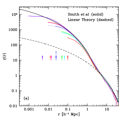
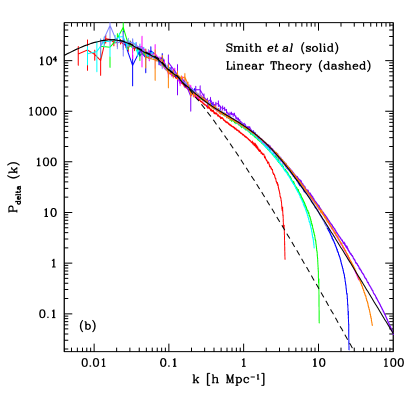
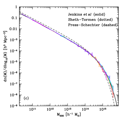
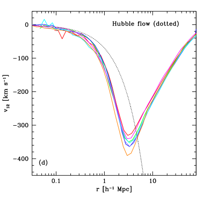
Figure 1: (a) Two point correlation function, (b) power spectrum, (c) mass function and (d) mean pairwise velocity. See color map in Table 1. The arrows in the top left panel indicate the gravitational softening. In the same panel, we also show the linear theory (dashed line) and the Smith et al (solid line) two-point correlation function fitting for the assumed cosmological model. The solid, dotted and dashed lines in panel (c) show the Sheth-Tormen, Jenkins et al and Press-Schechter ¹⁰ mass functions, respectively. Finally, in panel (d) the dashed line represents the Hubble flow.

Finally, Figure 1 (d) shows the mean pairwise velocity, $v_{12}(r)$, as function of pair separation. The Hubble line, given by $v_{Hubble}=-Hr$, is also shown. The mean pairwise velocity vanishes at the smallest separations resolved in our simulations. In the subset of simulations which better probe small scales (small volume and larger mass resolution) $v_{12}(r)$ closely follows the Hubble line up to $\sim 300$ kpc $h^{-1}$. This indicates that structures on such scales are close to relaxation. The mean pairwise velocity reaches a minimum in scales comparable to the correlation length [see Figure 1(d)]. At larger scales the $v_{12}(r)$ intersects the Hubble line and, at very large separations it decays to zero, in accordance with the principle of large-scale homogeneity and isotropy.

Some simulations in this suite have been further analyze in Seljak & Warren $\!{}^{{\bf?}}$.

References

References

- [1] U. Seljak & M. Zaldarriaga, ApJ. 469, 437 (1996)
- [2] M.S. Warren & J.K. Salmon, Supercomputing ’ 93, IEEE Comp. Soc., Los Alamitos 1993
- [3] R. Smith, J.A. Peacock, A. Jenkins, S.D.M. White, C.S. Frenk, F.R. Pearce, P.A. Thomas, G. Efstathiou, H.M.P. Couchman, MNRAS 341, 1311 (2003)
- [4] A. Jenkins, C.F. Frenk, F.P. Pearce, P.A. Thomas, J.M. Colberg, S.D.M. White, H.M.P. Couchman, J.A. Peacock, G. Efstathiou, A.H. Nelson, ApJ. 499, 20 (1998)
- [5] M.S. Warren & L. Teodoro, in preparation.
- [6] M. Davis, G. Efstathiou, C.S. Frenk and S.D.M. White, ApJ. 292, 371 (1985); D. Pfitzner, J. Salmon and T. Sterling, Journal of Data Mining and Knowledge Discovery 1, 419 (1977)
- [7] A. Jenkins, C.S. Frenk, S.D.M. White, J.M. Colberg, S. Cole, A.E. Evrard, H.M.P. Couchman, N. Yoshida, MNRAS 321, 372 (2001)
- [8] R. Sheth & G. Tormen, MNRAS 308, 119 (1999)
- [9] U. Seljak & M.S. Warren, ArXiv e-print astro-ph/0403698
- [10] W.H. Press & P. Schechter, ApJ. 187, 425 (1974)