Unified 1-D Simulations of Gamma-ray Line Emission from Type Ia Supernovae

Abstract

The light curves of Type Ia Supernovae (SN Ia) are powered by gamma-rays emitted by the decay of radioactive elements such as ⁵⁶Ni and its decay products. These gamma-rays are downscattered, absorbed, and eventually reprocessed into the optical emission which makes up the bulk of all supernova observations. Detection of the gamma-rays that escape the expanding star provide the only direct means to study this power source for SN Ia light curves. Unfortunately, disagreements between calculations for the gamma-ray lines have made it difficult to interpret any gamma-ray observations.

Here we present a detailed comparison of the major gamma-ray line transport codes for a series of 1-dimensional Ia models. Discrepancies in past results were due to errors in the codes, and the corrected versions of the seven different codes yield very similar results. This convergence of the simulation results allows us to infer more reliable information from the current set of gamma-ray observations of SNe Ia. The observations of SNe 1986G, 1991T and 1998bu are consistent with explosion models based on their classification: sub-luminous, super-luminous and normally-luminous respectively.

1 Introduction

Type Ia supernovae (SNe Ia) are intertwined with many of the most interesting frontiers of astrophysics. They occur in all galaxy types and are important contributors to galactic chemical evolution. They are very bright and their peak luminosities are relatively uniform. Furthermore, the variations in peak luminosity that do exist are related to the width of their luminosity peak (hereafter this relation will be referred to as the luminosity-width relation, or LWR). This relation has been both calibrated by estimating the distances to the host galaxies of nearby SNe Ia and simulated by performing radiation transport upon models purported to span the SN Ia event (Höflich & Khokhlov 1996, Pinto & Eastman 2000a, 2000b). The combination of an extremely bright luminosity peak and the relatively well-determined value of that peaks (via the empirical LWR) have permitted SNe Ia to be used as high-$Z$ distance indicators. Indeed, SNe Ia have been instrumental in establishing that the Hubble Constant (H₀) has a value of $\sim$ 70 km s^-1 Mpc^-1 (Freedman et al. 2001, Gibson et al. 2001) and in suggesting that the cosmological constant has a non-zero value (Perlmutter et al. 1999, Riess et al. 1998). These uses of SNe Ia proceed despite controversy as to the exact nature of SN Ia explosions.

Studies of the gamma-ray line emission from supernovae have long been recognized as a powerful way to probe the nucleosynthesis and explosion kinematics of these events (Clayton, Colgate & Fishman 1969, Ambwani & Sutherland 1988, Chan & Lingenfelter 1991). The ⁵⁶Ni $\rightarrow$ ⁵⁶Co $\rightarrow$ ⁵⁶Fe decay chain provides the most promising candidates for gamma-ray line studies of prompt emission from SNe, producing strong lines at 158, 812, 847 and 1238 keV. At early times, the line fluxes increase as the expanding ejecta unveils the radio-isotopes responsible for each line. The timing of this unveiling is a function of both the distribution of the isotopes and the kinematics of the ejecta. At later times, when the ejecta asymptotically approaches being optically thin to the gamma-rays, the line fluxes follow the isotopes’ decay curves and reveal the total production of each isotope. Neither of these line flux comparisons require an instrument capable of resolving the line. If the line can be resolved, measuring the line profiles of the individual lines shows the distribution (in velocity space) of the radio-isotopes in the ejecta, allowing a very precise probe of the nucleosynthesis in the SN explosion. Because of their low mass, thermonuclear supernovae (type Ia SNe) have very strong gamma-ray signals and gamma-rays make ideal probes of the type Ia SN mechanism.

As the shape of the light curve peak (important in calibrating SN Ia’s for use as cosmological probes) is a direct function of the ⁵⁶Ni decay chain, determining the distribution of ⁵⁶Ni in SNe Ia is a primary goal of SN Ia studies. At the elemental level, the same diagnostics used in gamma-ray line studies are also present in the optical and infra-red emission, and most current studies concentrate upon that wavelength range. However, optical and infra-red studies require a much more in-depth knowledge of the ejecta characteristics and suffer due to uncertainties in this knowledge. Gamma-ray emission studies have a number of features that allow a direct interpretation of the observations and a more exact estimation of the ⁵⁶Ni yield. The prompt emission lines from gamma-rays rely upon the production of one isotope (⁵⁶Ni) and the determined abundances do not suffer from line blends of a number of comparable isotopes as they do in the optical or infra-red. In addition, the dominant opacity for gamma-rays in the energy range of most gamma-ray lines is Compton scattering which varies smoothly with wavelength and depends only weakly on the composition. The gamma-ray emission lines are produced by the decay of ⁵⁶Ni and its decay product ⁵⁶Co which are insensitive to the ionization state of these isotopes. In contrast, the opacity in the optical and infra-red are dominated by a complicated combination of the line opacities from all the elements in the ejecta. Beyond the difficulty of merely including this forest of lines, the line opacities will depend sensitively both on the composition and ionization state of the ejecta. Gamma-ray emission is a much more straightforward, and ultimately more accurate, probe of the ⁵⁶Ni yield in supernovae.

Despite the promise of studying prompt emission, only three SNe Ia have even been observed with gamma-ray telescopes, resulting in only a single, weak detection (SN 1991T) and two upper limits (SNe 1986G and 1998bu). In fact, although the probability to detect prompt emission is predicted to be far higher for thermonuclear SNe than for core-collapse SNe, the two strongest detections have been from a SN of the latter type. SN 1987A was detected at 847 and 1238 keV (from ⁵⁶Co decays) by the SMM instrument (Matz et al. 1989) and with balloon-borne instruments (Mahoney et al. 1988, Rester et al. 1989, Teegarden et al. 1989, Tueller et al. 1990, Kazaryan et al. 1990, Ait-Ouamer et al. 1990), and at 122 keV (from ⁵⁷Co decays) by CGRO’s OSSE instrument (Kurfess et al. 1992).

Even so, the number of gamma-ray transport codes used in the literature to study SNe Ia exemplifies the importance of these diagnostics. Preliminary comparisons between these simulations reveal that the predicted fluxes vary considerably. Indeed, the variation caused by different codes was larger than the variation caused by different explosion models with the same code. Disentangling the differences between codes has been complicated by the fact that the work in the literature does not use the same set of supernova explosion models. In addition, most of the published work is limited to line fluxes, and different authors use different definitions of the line flux (i.e. whether the line flux results from the escape fraction of the photons in the specified line or from the convolution of an assumed instrument response over a simulated spectrum). In this paper, we eliminate the earlier confusion by directly comparing seven of the major codes used for gamma-ray line transport, using the same initial progenitors.

1) Müller, Höflich & Khokhlov (1991) and Höflich, Khokhlov & Müller (1992) simulated emission from delayed detonation models in anticipation of CGRO observations of SN 1991T. That on-going effort, utilizing the MC-GAMMA code, produced a number of papers, many of which studied the energy deposition in SN ejecta. A comprehensive paper by Höflich, Wheeler & Khokhlov (1998) explored various aspects of gamma-ray line emission, including displaying spectra, line fluxes, line ratios and line profiles for nine SN Ia models. More recently, they have also explored potential ramifications of asymmetry upon the line fluxes and line profiles of SN Ia emission (Höflich 2002). We include this code in our study, referring to it as “Höflich”.

2) Shigeyama, Kumagai, Yamaoka, Nomoto, & Thielemann (1991) simulated gamma-ray emission for two SN Ia models, including the 1991T model, W7DT. Kumagai followed up that work by simulating more models (including HECD) and treating the hard X/$\gamma$-ray emission from their models (Kumagai & Nomoto 1997, Kumagai, Iwabuchi & Nomoto 1999), and more recently by studying the supernova contribution to the cosmic gamma-ray background (Iwabuchi & Kumagai 2001). We include this code in our study, referring to it as “Kumagai”.

3) Other simulation efforts have been motivated by predicted performances of specific missions and/or studies of energy deposition in SN ejecta. Burrows & The (1990) studied X/$\gamma$-ray emission from SNe Ia in anticipation of the launch of the COMPTEL and OSSE instruments on the Compton Gamma Ray Observatory (CGRO), following earlier, similar studies of SN 1987A (Bussard, Burrows & The 1989, The, Burrows & Bussard 1990). That work investigated the energy deposition in SNe (The, Bridgman, & Clayton 1994), as well as the supernova contribution to the cosmic gamma-ray background (The, Leising & Clayton 1993). Milne, The, & Kroeger (2000) and Milne, Kroeger, Kurfess & The (2002) used simulated gamma-ray line fluxes of SN Ia models from this code to predict the performance of an Advanced Compton Telescope. We include this code in our study, referring to it as “The”.

4) Isern, Gomez-Gomar & Bravo (1996), Isern, Gomez-Gomar, Bravo & Jean (1997), and Gomez-Gomar,Isern & Jean (1998) all displayed results of an on-going study of gamma-ray emission from a range of SN Ia models. Those studies have concentrated upon the potential for the INTEGRAL satellite to detect that emission. We include this code in our study, referring to it as “Isern”.

5,6) Pinto, Eastman & Rogers (2001) employed the FASTGAM code to study the X/$\gamma$-ray emission from Chandrasekhar versus sub-Chandrasekhar mass models of SNe Ia. This code was first developed to study emission from SN 1987A (Pinto & Woosley 1988). The 3D Maverick code (Hungerford, Fryer & Warren 2003) was developed to study asymmetries in core-collapse supernovae. The physical processes included in Maverick were chosen to match those in FASTGAM, though the implementation techniques of these processes differed at the detailed level. We include the FASTGAM and Maverick codes in our study, referring to them as “Pinto” and “Hungerford” respectively.

7) In support of an effort to develop two next generation gamma-ray telescopes, an Advanced Compton Telescope (Boggs & Jean 2001) and a High-Resolution Spectroscopic Imager (Harrison et al. 2003), Boggs ($ApJ$ submitted) simulated line profiles for SN Ia models. We include this code in our study, referring to it as “Boggs”.

In Section 2, we introduce the simulation techniques employed by the seven groups and compare the physics that went into them. In Section 3, we compare the spectral results from all codes and describe what alterations were made to the codes to achieve agreement between all groups. In Section 4, we run a single code (The) with various models and compare the different results possible for different explosion scenarios. In Section 5, we compare these simulated spectra, with the SMM observations of SN 1986G and the COMPTEL & OSSE observations of SNe 1991T and 1998bu.

2 Decay and Transport Physics

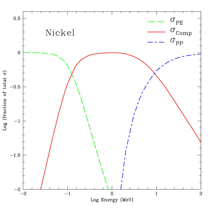
Figure 1: Cross sections for photon interactions in nickel. Compton scattering (solid line) dominates over photo-electric absorption (dashed line) and pair-production (dot-dashed line) over the energy range 0.1 - 10 MeV.

In order to understand the differences between the simulation techniques used by the various groups in this comparison, we must first lay out the basic physical picture of the problem we are representing numerically. For the purposes of determining the high energy spectrum (roughly 30 keV to 4 MeV) at the epochs of interest (10 to 150 days), the assumption of a homologously expanding supernova ejecta is valid. The ejecta composition includes radioactive species such as ⁵⁶Ni and ⁵⁶Co, the decay of which provides the $\gamma$-ray line photons that generate the line and, through scatter interactions, continuous $\gamma$-ray spectrum. The basic interaction processes involving these photons are pair production (PP), photo-electric (PE) absorption, and Compton scattering off free and bound electrons. Figure 1 shows a plot of cross sections for these interactions as a function of energy, which shows that the absorptive opacities, PE and PP, are only dominant at low ( $<150$ keV) and high ( $>10$ MeV) energies, respectively. The majority of the energy range discussed is dominated by Compton scattering interactions.

As discussed in detail by Ambwani & Sutherland (1988), the picture described above is well-suited for Monte Carlo transport methods. Since six of the seven groups in our collaboration have employed this technique (Höflich, Hungerford, Isern, Kumagai, Pinto and The), we briefly recap the major points described by Ambwani & Sutherland (1988). The fundamental advantage of Monte Carlo is its ability to accommodate very complicated physical processes in the transport. This is accomplished by simulating the micro-physics of the photon’s propagation through the supernova ejecta. The principle is very straightforward: the mass of nickel atoms in the input model implies a certain amount of radioactive decay luminosity. Monte Carlo packets (which represent some quantum of photon luminosity) are then launched in proportion to the decay rate and the mass distribution of nickel atoms. Each packet’s energy is chosen in proportion to the branching ratios of the possible decay lines and its initial direction is picked at random, assuming isotropic emission. The emitted packet is then allowed to propagate through the ejecta, interacting with the material through scattering and absorption. This is a microscopic treatment of the transport in the sense that each individual packet of photons is tracked through each individual interaction.

The likelihood of a photon experiencing an interaction during its flight is dictated by the total cross section for interaction ($\sigma_{tot}$). When an interaction occurs, the type of interaction, scatter or absorption, is chosen randomly in proportion to the ratio of $\sigma_{scat}/\sigma_{tot}$ or $\sigma_{abs}/\sigma_{tot}$. The well-described micro-physics of the PP and PE absorption and the Compton scatter process are explicitly taken into account for each packet interaction, and are thus treated with no approximation. When a packet’s path brings it to the surface of the ejecta, it is tallied into the escaping SN spectrum. Likewise, if the path ends in an absorption, the packet’s energy is deposited into the ejecta. In this way, the Monte Carlo transport technique allows for straightforward calculation of the emergent hard X- and $\gamma$-ray spectrum, as well as energy deposition into the ejecta via photon interactions.

If the emerging line profile of the $\gamma$-ray decay lines is the only quantity of interest, semi-analytic techniques alone, as employed by Boggs in this comparison, can be effectively used as well. The Compton equation describes the energy shift a photon experiences upon suffering a Compton scatter. For the decay lines we are interested in (E$\sim$1 MeV), a single Compton scatter generally shifts the photon’s energy out of the decay line profile. This means that the line profiles in the emergent spectrum arise primarily from photons that escape the ejecta without any interaction, with a secondary contribution from forward-scattered Compton photons. The line profiles can thus be calculated analytically by multiplying the emitted luminosity, as determined from the mass distribution of radioactive species in the ejecta, by the factor $e^{-\tau}$, where $\tau$ is the total optical depth from the emission point to the surface of the ejecta. Analytical techniques such as this provide an invaluable test of the more computationally intensive Monte Carlo technique described above.

Regardless of technique chosen, bringing the physical picture to a numerical representation requires a series of computational decisions. In the following sub-sections we will review the physics pertinent to these computational choices. These choices fall into three primary categories:

• Description of the Ejecta (Differential Velocity, Density Evolution)

• Photon Source Parameters (Lifetimes and Branching Ratios, Positron Annihilation, Ejecta Effects, Weighting)

• Opacities for Photon Interactions (Compton Scattering, Photo-Electric Absorption, Pair Production and Bremsstrahlung Emission)

Table 1 lists the various codes and provides information regarding the numerical implementations of the physics discussed below.

2.1 Ejecta

For the different explosion models, the ejecta is determined by mapping the model into spherical Lagrangian mass zones and expanding this ejecta homologously outward with time. Taking snapshots in time of this ejecta, each gamma-ray calculation uses the density, radius, velocity and composition of the ejecta for these mass zones. Some codes simply take the position of the ⁵⁶Ni and ⁵⁶Co, but others include the motion of the ejecta at varying levels of sophistication. The two major velocity effects are the differential motion and the density reduction due to expansion.

2.1.1 Differential Velocity

Since the radioisotope is distributed in velocity space and the opacity depends on the relative velocities, the ejecta velocity will affect the propagation of the photon packets. The packets are created with a decay line energy in the co-moving frame of the surrounding ejecta, but are tallied in the rest frame of the observer. The Doppler shift between these two frames is the dominant source of broadening in the line profiles. In Figure 2, we show the amount of line broadening possible for four SN Ia models. In addition, as the packet propagates through the ejecta, its energy, as measured in the local co-moving ejecta frame, is constantly changing. Since interaction cross sections are energy-dependent, the opacity through the ejecta for the packet will be different from the case where ejecta velocity is neglected. For our scenario, this is a small effect, as our dominant opacity (Compton scattering) is a slowly varying function of energy.

The Boggs, Höflich, Hungerford, Isern and Pinto algorithms included the ejecta velocity effects, allowing them to calculate detailed line profiles (Table 1).

2.1.2 Density Evolution

Assuming the decision was made to account for ejecta velocity effects, one must then choose whether to allow this motion to feed back on the densities throughout the ejecta. The photon packet does not traverse its path infinitely quickly. Indeed, there is some flight time associated with each packet trajectory, and during this flight time, the ejecta undergoes expansion. This results in lower densities, and thus lower opacities, as the packet propagates through the star. The alternative to treating this expansion is to assume the transport takes place within a differential time slice $dt$, over which the hydrodynamic quantities do not evolve at all. For a homologously expanding ejecta, the density falls off simply as $t^{-3}$, making this feedback effect easy to implement. However, accounting for it is only a partial step toward a time-dependent treatment of the problem. The source of the photon packets must also be treated in a time-dependent fashion in order to be self-consistent. Unfortunately, the implementation of the source’s time-dependence is not trivial in a Monte Carlo treatment.

Pinto allowed for the ejecta expansion to feedback on the densities. The semi-analytic technique employed by Boggs accounted for both the expansion feedback and the time dependence of the photon source (i.e. photons from the far side of the ejecta take longer to arrive at the detector and must be launched at an earlier time during the explosion. See §2.2.3)

2.2 Photon Source

Differences in the gamma-ray sources include not only ⁵⁶Ni and ⁵⁶Co decay times and branching ratios, but the emission from positron annihilation. The actual photon emission also depends on the ejecta. Finally, the method of weighting the packets can also pose a problem when normalizing the escaped packet counts into physical flux units.

2.2.1 Decay Times and Branching Ratios

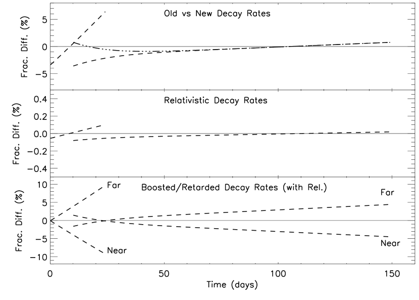
Figure 3: Nickel and Cobalt decay rates. The upper panel shows the fraction change in the decay rates for ⁵⁶Ni and ⁵⁶Co assuming 8.8^d and 113.7^d mean lifetimes rather than 8.5^d and 111.5^d (dashed lines). The simplified ⁵⁶Co decay rate used in HWK98 compared with the 8.5^d and 111.5^d lifetimes is also shown (dot-dot-dot-dashed line). The middle panel shows the fractional change in the decay rates produced by considering the relativistic effects of the ejecta’s expansion velocity upon the decay rates. The lower panel shows the effect of the boosting/retarding of the decay rate to synchronize all photons to arrive simultaneously with photons from the center of the SN ejecta. The ejecta velocity is assumed to be 10,000 km/s in the lower two panels, a relatively large value for ⁵⁶Ni-rich ejecta. Bear in mind that until the ejecta becomes thin to gamma-rays, the emission from the decays near the surface on the near edge will dominate the integrated emission.

The source of photons for these high energy calculations is exclusively $\gamma$-ray line emission from the decay of various radio-isotopes present in the supernova ejecta. The fundamental decay chain is that of the radio-isotope ⁵⁶Ni. The SN explosion synthesizes ⁵⁶Ni, which promptly decays via electron capture to ⁵⁶Co with a mean lifetime of $\sim$8.8 days. The ⁵⁶Co produced in this decay is also unstable, though with a longer lifetime ($\sim$111.4 days). However, we expect the errors caused by the decay times to be less than $\sim$5% (Figure 3).

Whereas the ⁵⁶Ni decay always proceeds via electron capture, the ⁵⁶Co decay proceeds either through electron capture (about 81% of decays) or positron production (roughly 19% of decays). Shown in Table 2 are the relative abundances of the dominant lines from the ⁵⁶Ni and ⁵⁶Co decays. Note that these values refer to the number of photons emitted per 100 decays of the respective isotope (i.e. this includes the effects of the 19% positron production branching ratio). Clearly, the dominant branches, both for studies of gamma-ray line emission and for studies of the energy deposition are the 158, 812, 847 and 1238 keV lines. The exact values for branching ratios and lifetimes of these radioactive decays are subject to updates and revisions, as one might expect. As a result, the suite of values used in a $\gamma$-ray transport code are chosen from a range of possibilities available in the refereed literature.

For the most part, the values adopted from different references have no noticeable affect on the calculated spectra. The only significant variations in adopted branching ratios from earlier works to the current simulations was with the Höflich code. In previous works, the Höflich code adopted 0.74 for the 812 keV line of ⁵⁶Ni decay rather than the 0.86 employed by the other groups. Also, in previous simulations with the Höflich code, it was assumed that the positron production branch left the ⁵⁶Fe daughter nucleus always in its ground state (Müeller, Höflich, Khokhlov 1991). This led to branching ratios for the $\gamma$-ray lines from excited ⁵⁶Fe being reduced from the published values by the 19% positron production branching ratio.

2.2.2 Positron Decay

Absent from Table 2 are the 511 keV line and positronium continuum which result from the positron production branch of the ⁵⁶Co decay. These positrons are created with $\sim$ 600 keV of kinetic energy that must be transferred to the ejecta before the positron can annihilate with electrons in the ejecta. It is usually assumed that during the epoch of interest for gamma-ray line studies ($\leq$ 150 days), positrons thermalize quickly and thus have negligible lifetimes, annihilating in-situ. Detailed positron transport simulations (Milne, The & Leising 1999) have shown that this is not a wholly correct assumption at 150 days; however, only a small error is introduced by making this assumption. Although it is reasonable to assume that the positrons annihilate promptly, in-situ, the nature of the resulting emission is not clear. Depending upon the composition and ionization state of the annihilation medium, the positron can annihilate directly with an electron (and produce two 511 keV line photons in the rest frame of the annihilation), or it can form positronium first. If positronium is formed (and the densities are low enough to not disrupt the positronium atom), 25% of the annihilations occur from the singlet state. Singlet annihilation gives rise to two 511 keV line photons, as with direct annihilation. However, 75% of annihilations occur from the triplet state, which gives rise to three photons. As the three photons share the 1022 keV of annihilation energy, a continuum is produced. This continuum increases in intensity up to 511 keV and abruptly falls to zero.

The resulting spectrum can thus be characterized by the positronium fraction, f(Ps), a numerical representation of the fraction of annihilations that form positronium (e.g. Brown & Leventhal 1987):

$$f(Ps)=\frac{2.0}{1.5+2.25(A_{511}/A_{posit})},$$ (1)

where $A_{511}$ and $A_{posit}$ are the observed 511 keV line and the positronium three-photon continuum intensities, respectively. Positronium fractions range between 0 - 1, with most researchers assuming that SN annihilations have a similar positronium fraction as the Galaxy. Utilizing wide-FoV TGRS observations of galactic positron annihilation, Harris et al. (1998) estimated the positronium fraction to be 0.94$\pm$0.04. Similarly, utilizing CGRO/OSSE observations of the inner Galaxy, Kinzer et al. (2001) estimated the positronium fraction to be 0.93$\pm$0.04, both values in agreement with theoretical estimates of interstellar medium (ISM) positron annihilation. However, the composition of SN Ia ejecta is far different than the ISM, being dominated by intermediate and heavy elements rather than hydrogen and helium. Thus, ISM annihilation is completely different than SN ejecta annihilation. Likewise, the galactic annihilation radiation measured by OSSE is a diffuse emission, and thus it is distinct from the in-situ annihilations that occur in SN Ia ejecta within 200 days of the SN explosion. The expectation is that charge exchange with the bound electrons of these intermediate and heavy elements would lead to SN ejecta having a positronium fraction of at least 0.95. However, a zero positronium fraction for annihlations that occur in SN ejecta cannot be ruled out.

For our purposes here, it suffices to say that the expected spectrum from positron annihilation is uncertain, and the individual members of this comparison team have adopted positronium fractions of either 0 (Hungerford, Kumagai, and Pinto) or 1 (Höflich, Isern, and The); see Table 1 for a summary. The three groups employing positronium fractions of 1 adopted the energy distribution of the positronium continuum treatment in Ore & Powell (1949).

2.2.3 Ejecta Effects on Decay

The motion of the ejecta can also change the decay rate. The decay equations for ⁵⁶Ni and ⁵⁶Co decays in a stationary medium are:

$$\frac{1}{{\mathrm{Ni}}_{o}}\left(\frac{dNi}{dt}\right)=-\frac{1}{\tau_{Ni}}exp\left(\frac{-t}{\tau_{Ni}}\right),$$ (2)

$$\frac{1}{{\mathrm{Ni}}_{o}}\left(\frac{dCo}{dt}\right)=\frac{-1}{\tau_{Co}-\tau_{Ni}}\left[exp\left(\frac{-t}{\tau_{Co}}\right)-exp\left(\frac{-t}{\tau_{Ni}}\right)\right],$$ (3)

where, $\tau_{Ni}$ and $\tau_{Co}$ are the mean lifetimes of the isotopes, Ni_o is the ⁵⁶Ni produced in the SN explosion, and $t$ is the time since explosion. For a given model time ($t=t_{m}$), these equations can be solved for the number of Nickel and Cobalt atoms that will decay during an infinitesimal time slice $dt$. These equations still hold for a finite time step $\Delta t$, assuming $\Delta t$ is much less than the lifetime $\tau$. Strictly speaking, the lifetimes ($\tau_{Ni}$ and $\tau_{Co}$) in the above equations, are in the frame of the isotope, which is moving relative to an external observer. Since the velocity of the ejecta can be upwards of 10,000 km s^-1, an exact treatment of the decay rate must include a conversion to the frame of the external observer. This relativistic effect is proportional to $\gamma=(1-v^{2}/c^{2})^{-1/2}$ and is only a 0.1-0.2% effect overall (Fig. 3). Aside from Boggs, none of the codes include this effect.

More important is the flight time of the photons through the ejecta. In the context of Equations (2) and (3) it is straightforward to point out where to accomplish this. Emission from the near side of the ejecta should be calculated from the above equations using a retarded time relative to the far side. In this way, photons from the front and back of the ejecta arrive simultaneously at the detector. Figure 3 shows the effect these two issues (in the extreme) have on the calculated decay rate. The flight time of the photons introduces less than a 10% error. (N.B. The dash-dot-dot line in Figure 3 represents the variation in decay rate of Cobalt resulting from an approximate form of Equation 3 used in one of the comparison codes.) Again, Boggs’ code is the only one that incorporates these effects.

2.2.4 Weighting

The last uncertainty is purely numerical in nature and arises from the weighting (and subsequent normalization) of the photon packets. Combining the decay rate with the branching ratios, which provide a measure of the average number of photons per decay, Equations (2) and (3) yield a total photon luminosity (${\mathcal{L}}_{phot}$) of the ejecta (in phot/s). Given the number of photon packets to be tracked in the simulation (${\mathcal{N}}_{packet}$), the weight of each packet is

$${\mathcal{W}}_{packet}=\frac{{\mathcal{L}}_{phot}}{{\mathcal{N}}_{packet}}.$$

More complicated weighting algorithms are possible, and provide advantages when specialized information is desired. For example, detailed studies of the spectral characteristics for weaker decay lines benefit from emitting a large number of packets at the decay energies of interest. In this way, the signal-to-noise of the spectrum at those weak lines is enhanced beyond what the uniform weighting technique could provide. In any case, the normalization applied via this weight factor can be taken into account from within the transport code itself, or as a post-process step on the photon packet counts, which result from the base Monte Carlo transport routine. The validity of the normalization is easily tested through the analysis of the integrated line flux lightcurves for the various decay lines. These lightcurves can be directly compared with the semi-analytic technique discussed above for decay lines with energies greater than about 1 MeV (i.e. where the continuum has a negligible contribution to the spectrum.) For our study, all the Monte Carlo algorithms were run using constant weight packets to reduce the complexity of the comparison, but as we shall see, it is the weighting and the subsequent normalization of the flux that caused many of the discrepancies in past simulations (see §3.4).

2.3 Photon Interaction Processes

Once the decay photons have been created, their propagation through the ejecta is dictated by the three interaction processes mentioned at the start of this section: Pair-Production, Photo-Electric absorption and Compton scattering. The major features of the spectrum, with the exception of actual line fluxes, can be understood primarily through the PE absorption and Compton scatter interactions.

2.3.1 Compton Scattering

For the majority of the energy range we are interested in, the Compton scatter interaction off bound and free electrons dominates. This interaction depends only on the total electron density in the ejecta and energy of the incident photon. Since almost all SN Ia ejecta has an electron fraction Y_e $\sim$ 0.5, this interaction is only weakly dependent upon the composition.

Figure 1 shows the energy dependence of the cross-section for Compton scattering as employed by the various groups. This cross-section is a smoothly varying function of energy and, in general, is represented

$$\sigma_{\rm Compton}=\frac{3\sigma_{Th}}{8\epsilon}\left[\left[1-\frac{2(\epsilon+1)}{\epsilon^{2}}\right]{\mathrm{l}n}(2\epsilon+1)+\frac{1}{2}+\frac{4}{\epsilon}-\frac{1}{2(2\epsilon+1)^{2}}\right],$$ (4)

where $\sigma_{Th}$ is the Thomson scattering cross-section, and $\epsilon$ is the ratio of the photon energy to the electron rest mass.

While photo-electric absorption and pair-production interactions consume the photon, the scattering process produces a lower energy photon traveling in a new direction. The down-conversion of the photon’s energy is the dominant process for populating the hard X-ray continuum, and the exact energy distribution of the outgoing photons is described by the Klein-Nishina (KN) differential scatter cross-section. The KN formula is given by (Raeside, 1976)

$$\frac{d\sigma}{d\epsilon^{\prime}}=-\frac{3\sigma_{Th}}{8}\left(\frac{1}{\epsilon}\right)^{2}\left[\frac{\epsilon}{\epsilon^{\prime}}+\frac{\epsilon^{\prime}}{\epsilon}-1+\left(1-\frac{1}{\epsilon^{\prime}}+\frac{1}{\epsilon}\right)^{2}\right],$$ (5)

where $\epsilon$ is the photon’s incoming energy and $\epsilon^{\prime}$ is the photon’s outgoing energy. Given $\epsilon$, many techniques exist for sampling an outgoing energy from this relation. Combining this information with the Compton formula, an outgoing photon direction is then determined. Detailed comparisons of the individual sampling techniques used by the various groups have not been done. However, for the six groups that track the scattered photons, the continuum in their simulations is produced entirely through the scatter interaction. Fortunately, the shape of this Comptonized continuum (200 keV - 800 keV) is a direct and sensitive test that the physics of photon-electron scattering has been implemented appropriately.

2.3.2 Pair-Production and Photo-Electric Absorption Opacities

At low energies (less than $\sim$ 200 keV), the smooth, nearly power law continuum created from Compton scattering suffers a turn over due to photo-electric absorption effects. Just as in the adoption of values for branching ratios and decay lifetimes, the literature offers more than one reference for choosing absorptive opacities. The PE and PP opacities employed by the various groups in our collaboration can be found from three primary references (Viegle, Hubbell and ENDL), which provide these cross sections in tabular form (by energy and proton number.) Techniques for interpolating cross sections from the provided energy table values varied among the different groups. The number of nuclei species (different proton numbers), which were considered as contributors to these absorptive opacities, were also treated differently in the various codes. These types of variations in the numerical implementation ought to manifest themselves as slight changes in the location of the low energy spectral cut off.

In addition, both of these absorptive interactions allow for the possibility of high energy photon daughter products: annihilation photons for the case of pair production, and X-ray fluorescence photons for the case of photo-electric absorption. The decision to include these processes and the technique for implementing them varied among groups. The X-ray fluorescence photons are below the low energy cutoff and, thus, contribute predominantly to the calculated deposition energy. In this paper we concentrate only on the emergent spectrum, and thus do not probe the differences caused by the inclusion of the X-ray fluorescence.

2.3.3 Bremsstrahlung Emission

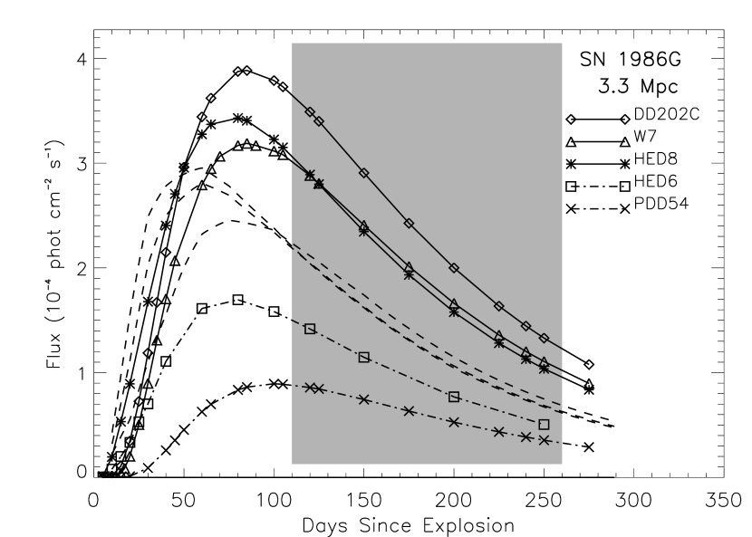
Figure 13: Five current simulations of 847 keV line emission from SN Ia models at 3.3 Mpc compared with 3$\sigma$ upper limit light curves derived from SMM observations of SN 1986G (Matz and Share 1988). The three Matz and Share light curves are shown with dashed lines, the five current simulations are identified as shown. The epoch of maximum SMM angular response to SN 1986G is shaded. The normally-luminous models appear too bright at the 3$\sigma$ level, while the very sub-luminous models are acceptably faint.

Another important photon emission process from the ejecta is the bremsstrahlung process of the energetic Compton-recoil electrons (E $\leq$ 3 MeV; recoiling from Compton scattering events with the primary radioactivity gamma rays). This bremsstrahlung process takes place in all supernovae that are powered by radioactive decay. The large abundance of these electrons gives rise to the dominance of bremsstrahlung photons as the hard X-ray source; i.e., below 30 keV and 60 keV at 20^d and 80^d, respectively in both models W7 and DD4 (Clayton & The 1991; Pinto, Eastman, & Rogers 2001). The shape of the bremsstrahlung spectrum emerging from the surface is sensitive to the photoelectric opacity and with the flux, $F(E)\propto E^{\alpha}$ where $\alpha$ is $\sim$1.1 and $\sim$1.8 at 20^d and 80^d, respectively for model W7 (Fig. 13 of Clayton & The 1991); the spectral luminosity increases slowly between 1 and 60 keV. The sudden change in the hard X-ray slopes between 10 keV and 100 keV (from the bremsstrahlung spectrum at lower energies to the Compton scattering spectrum at higher energies) can be used as the signature of this process. None of the simulations in this comparison project included this process.

3 Comparisons between Codes

The seven codes included in this study have all produced published simulations of SN models. All but the Hungerford code have produced published simulations of specifically SNe Ia. Indirect comparisons between published works from the codes being studied in this paper suggest that different codes reach different answers. Notably, HWK98 and Kumagai & Nomoto (1997) both predict larger line fluxes than Pinto, Eastman & Rogers (2001), Milne, Kroeger & The (2001) or Boggs ($ApJ$ submitted). However, determining the cause of such spectral variations has been difficult since no single input Ia model has been simulated by all groups. While it is generally agreed that SNe Ia are caused by the thermonuclear explosion of an accreting WD, there remains considerable controversy as to the exact nature of the progenitor and the physics behind the development of the burning front: deflagration vs. detonation, number of ignition sites (e.g. Livio 2000). These differences have produced a set of SN Ia explosion models in terms of a handful of parameters that form the basis for comparisons with SN observations. In this paper, we provide the much needed direct comparisons by running all seven gamma-ray transport codes on the same set of SN Ia explosion model inputs. The set of three models that were selected for comparisons are DD202C (a Chandrasekhar-mass delayed detonation, Höflich, Wheeler & Thielemann 1998), HED6 (a sub-luminous, sub-Chandrasekhar mass Helium detonation, Höflich & Khokhlov 1996) and W7 (a Chandrasekhar-mass deflagration, Nomoto, Thielemann & Yokoi 1984). In Table 3, we show the relevant characteristics of the models. Errors were introduced by imperfections in the conversion of each model into the varied formats required by each code. Typically these errors were 2-3% of the mass or kinetic energy and were found to have a negligible effect upon the Compton-scattering dominated portion of the spectra.

For these comparisons, we focus on three aspects of the gamma-ray calculations: the overall spectra, the line profiles and, the most-important observed quantity in the near future, the line flux.

3.1 Overall Spectra

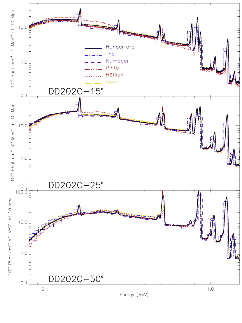
Figure 4: A sequence of spectra for the SN Ia model, DD202C. The spectra, at 15^d, 25^d, and 50^d, show the level of agreement between simulations for both the line and continuum emission. Comparisons between the two algorithms that do not treat line broadening/shifting (The & Kumagai) and the others that do, show the early effects of blue-shifting.

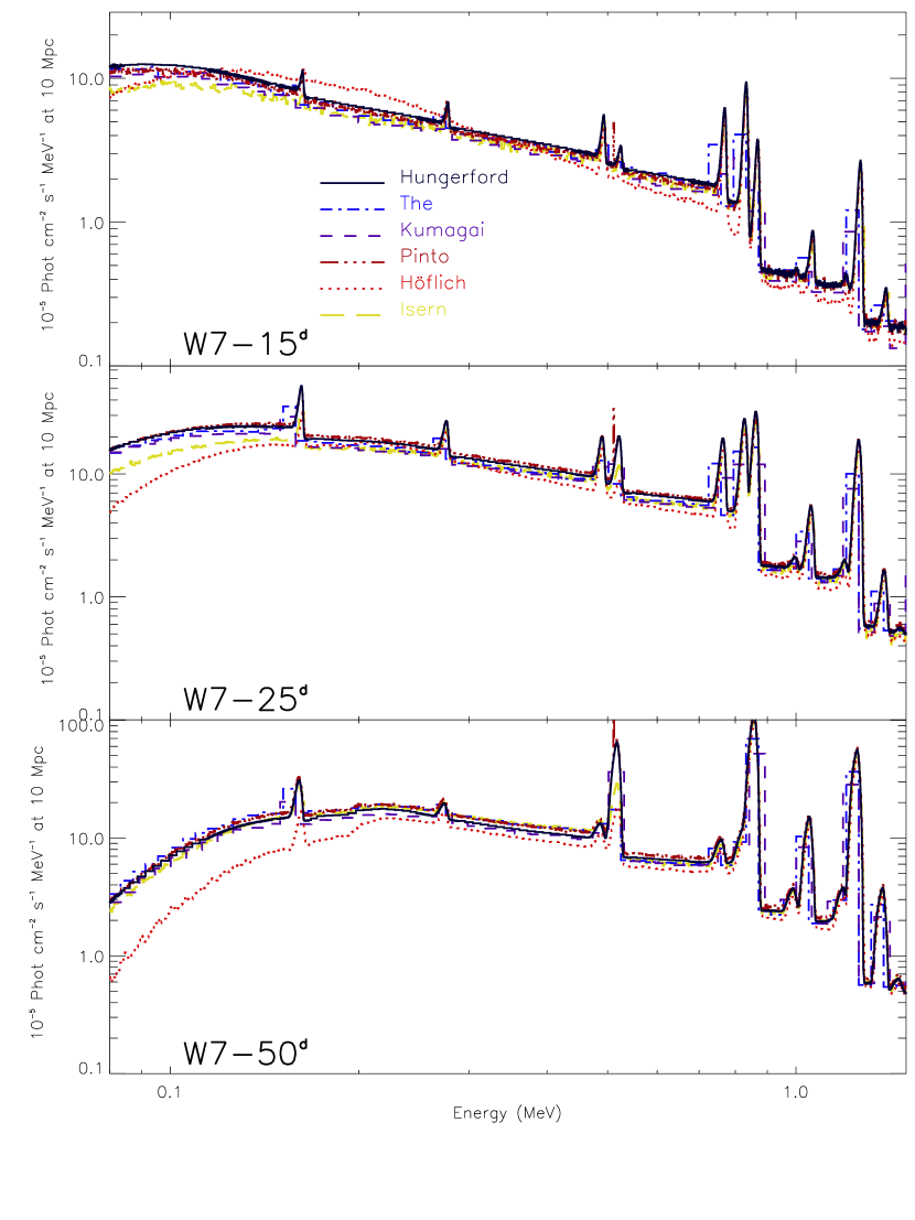
Figure 5: A sequence of spectra for the SN Ia model, W7. The absence of nickel near the surface of W7 leads to the inhibition of line emission until later times. As with DD202C, the spectra, at 15^d, 25^d, and 50^d, show a high level of agreement between simulations for both the line and continuum emission.

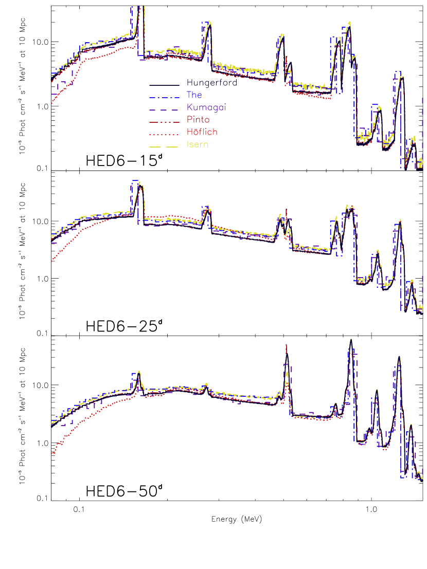
Figure 6: A sequence of spectra for the SN Ia model, HED6. The spectra, at 15^d, 25^d, and 50^d, show a high level of agreement between simulations, in this case for a low-mass model that features early escape of gamma-ray emission.

Figures 4 - 6 show a sequence of spectra from simulations of DD202C, W7, and HED6, respectively. These spectral results arise from current versions of the 6 Monte Carlo codes employed in this comparison and agree to within the statistical noise except in a few cases. $\S$3.3 describes in detail the necessary corrections that were made to arrive at the current versions. The remaining differences in the spectral simulations can be isolated in terms of the physical processes outlined in $\S$2. For example, in Figures 4 and 5 at the earliest epoch, it is clear that the Höflich spectra exhibit a different continuum slope across the rough energy range of 200 keV - 800 keV. The shape of the continuum in this portion of the spectrum is dictated primarily by the Klein-Nishina differential scattering cross section, although physical effects such as Doppler corrections for the ejecta velocities may also change the overall spectral slope. Closer inspection of the Compton scatter and Doppler boost routines between Höflich and other codes did not reveal an obvious cause for this difference, which has a maximum magnitude of order 30% but is much smaller across most of the energy range.

As discussed in $\S$2.2.2, spectral variations due to differences in the assumed positronium fractions should appear in the 400 - 550 keV energy range (Figures 4 - 6). At late times, one would expect the codes that include the positronium continuum to have slightly higher continuum spectra and weaker lines. There is very little difference between the codes that include a positronium continuum component (Höflich, Isern, and The) and those that do not (Hungerford, Kumagai, and Pinto), but the expected trends seem to hold. As these spectra likely bracket the range of possible annihilation spectral features, the treatment of the positronium fraction primarily affects the strength of the 511 keV line, and it does not dominate the appearance of the continuous spectrum.

There also remain differences in the $\leq$ 100 keV spectra that exceed statistical fluctuations. These differences likely arise from differences in the implementation of photoelectric absorption opacities. Differing interpolation techniques for the tabular opacities, to account for the difference in number of nuclear species treated, may be responsible for these discrepancies. As the emphasis of this comparison is on the higher energy gamma-ray portion of the spectrum, we did not attempt to resolve these opacity differences.

3.2 Line Profiles

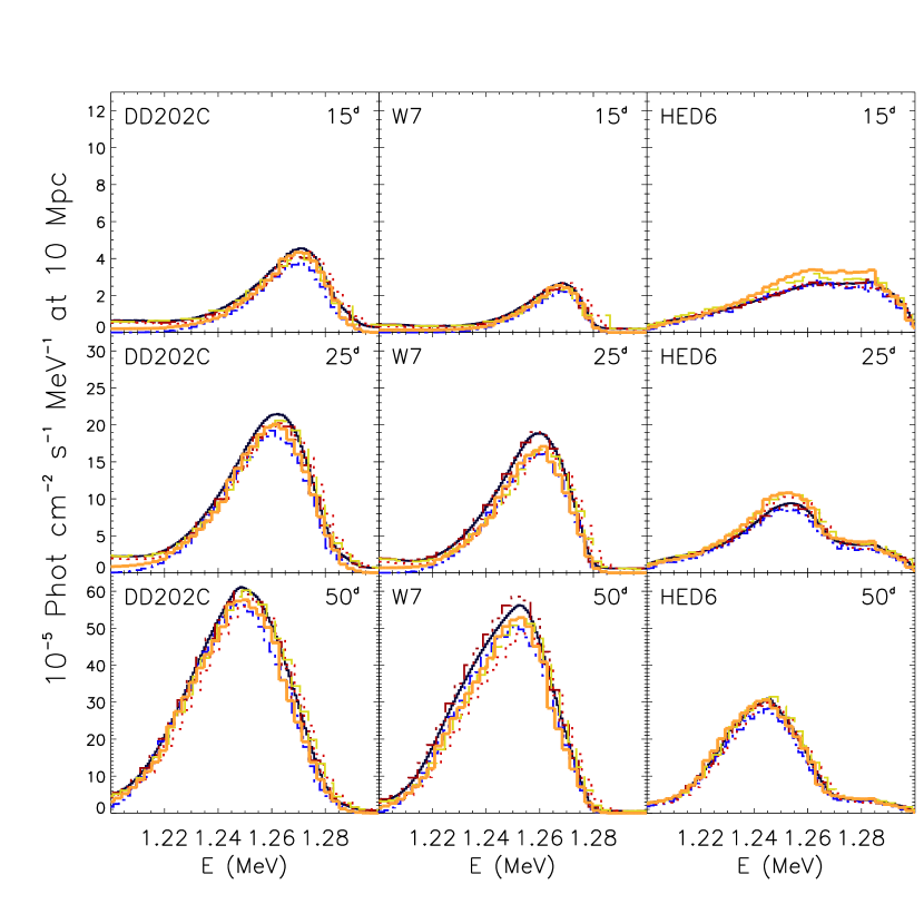
Figure 7: Line profiles of the 1238 keV line for the SN Ia models, DD202C, W7, HED6. Although the simulations show noticable variations, the differences between the Chandrasekhar-mass models (DD202C & W7) and the sub-Chandrasekhar-mass model (HED6) greatly exceeds the variations between simulations. Differentiating between DD202C & W7 is more difficult, but is not rendered impossible by the variations between simulations if a sequence of spectra were available for comparison.

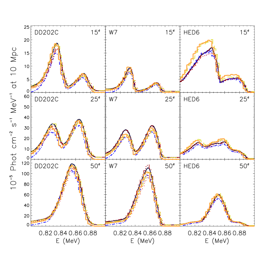
Figure 8: Line profiles of the 812 & 847 keV line complex for the SN Ia models, DD202C, W7, HED6. The interpretation is similar to that of the 1238 keV line: the differences between the Chandrasekhar-mass models (DD202C & W7) and the sub-Chandrasekhar-mass model (HED6) greatly exceeds the variations between simulations, and while differentiating between DD202C & W7 is more difficult, it is not rendered impossible by the variations between simulations if a sequence of spectra were available for comparison.

In Figures 7 and 8 we show line profiles of the 1238 keV line and the 812 & 847 keV line complex. The Boggs simulations are specifically of line profiles, and thus they contribute only to these two figures and not the previous three. The Kumagai and The codes did not produce line profiles and are thus not included in these figures. We note that Burrows & The (1990) did simulate line profiles by adopting a technique explained in Bussard et al. (1989), which is similar to the technique explained in Chan & Lingenfelter (1987).

The Boggs line profiles, shown in Figures 7 and 8, do not include the Compton scattered photons from higher energy nuclear lines. The fact that the Boggs line profiles agree very well with the other line profiles suggests that treating the Compton downscattered photons has only a small effect on the line profiles. These photons would only become important if an instrument’s energy resolution is poor enough that it samples beyond the energy ranges shown in these figures.

Although detailed line profile observations require instrument sensitivities beyond those currently available (for all but the nearest supernovae), their diagnostic potential for distinguishing between Ia explosion models is very strong. Because the line photons arise primarily from non-interacting gamma-rays, the line shape is a direct probe of the spatial distribution of ⁵⁶Ni synthesized in the supernova explosion. For a more detailed discussion of the potential for such observations with current and planned missions, see HWK98.

3.3 Line Fluxes

A far easier observation to make, and the quantity more frequently published from theoretical simulations, is the time evolution of integrated line fluxes (gamma-ray light curves). Since the Kumagai and The codes do not include ejecta velocity effects, they compare line emission with the other codes only through integrated flux values, obtained by tallying “tagged” line photons (i.e. a photon created at the gamma-line energy is tagged as such and contributes to the integrated flux if it escapes with no interaction).

Such comparisons of the lightcurves from previously published results in HWK98 (for DD202c and HED6) revealed significant differences in the magnitude and shape of the 812, 847 and 1238 keV lightcurves from the results presented here. Further inspection of the overall spectra from HWK98 confirmed that the spectra were similar in shape, but tended to be brighter by an epoch-dependent factor. Closer study of the Höflich code determined that a post-process step, required for correct weight normalization of the Monte Carlo packets, was performed incorrectly in the HWK98 spectra. (For details, see erratum for Höflich, Wheeler & Khokhlov 1998, in press.) When corrected for the appropriate weight factor, which was equal to the total escape fraction for each epoch, the HWK98 spectra roughly agree with the spectral results in this work.

Lightcurve results from Kumagai & Nomoto (1997) for model W7 also demonstrated an enhanced flux level, although the lightcurve shape was similar to the results found here. Comparisons with previously published W7 spectra (Kumagai & Nomoto 1997; Kumagai, Iwabuchi & Nomoto 1999; Iwabuchi & Kumagai 2001) reveal consistent results with the overall spectra presented in $\S$3.1. This points to an offset problem in the generation of the integrated flux data, possibly related to setting the SN at a given distance and/or scalings in the ⁵⁶Ni mass of the explosion model.

3.3.1 1238 keV Line Flux

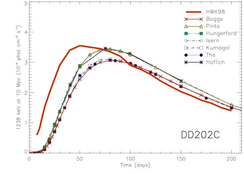
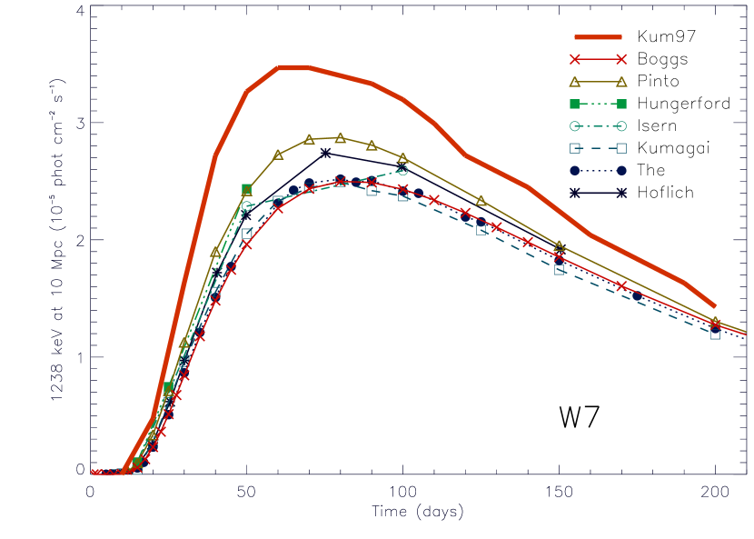
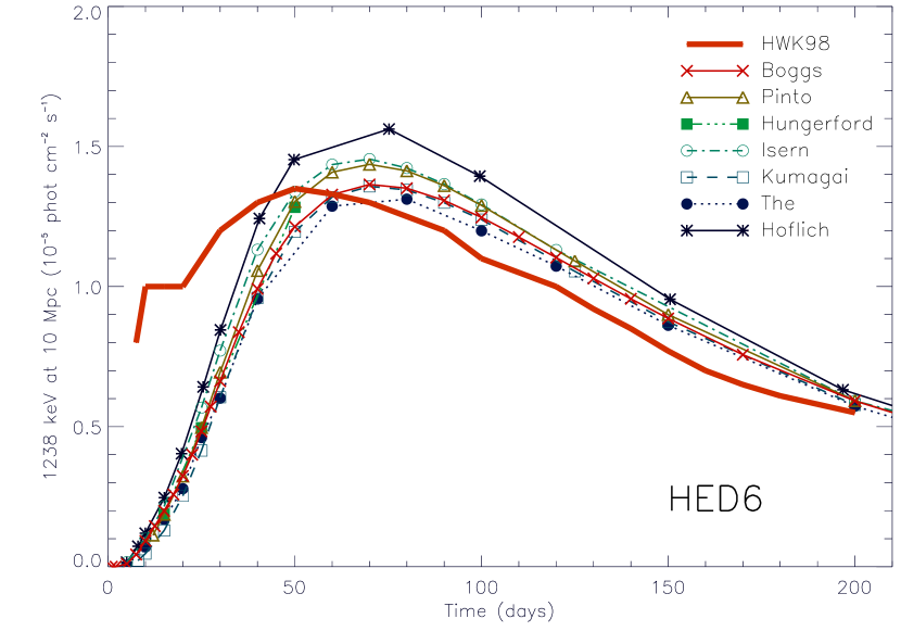
Figure 9: Line fluxes of the 1238 keV line for the SN models, DD202C (upper panel), W7 (middle panel) and HED6 (lower panel). The line fluxes extracted from the spectra (Höflich, Maverick, Fastgam, Isern) agree with the line fluxes that result from tagging line photons (The, Boggs, Kumagai). All current simulations predict fainter light curves than shown in previous published results (HWK98 for DD202C & HED6; Kumagai 1997 for W7). Spectral extraction assumed a 1150 - 1300 keV bandwidth. The HWK98 results are shown with and without the scaling for the escape fraction and branching ratios. Although the line definition in HWK98 differs from that used in this work, the light curves are similar when the corrections are applied.

The 1238 keV ⁵⁶Co decay line is the most straightforward line flux to study. This line is isolated from other lines and there is little continuum emission to contaminate line flux estimates. We define the 1238 keV line to be all photons with energies between 1150 - 1300 keV. Shown in Figure 9 are the 1238 keV light curves for DD202C, W7 and HED6. For comparison, we include earlier light curves from HWK98 and Kumagai & Nomoto (1997), although those works did not use the same line definitions used in this work.

The HWK98 light curves (DD202c and HED6) are enhanced at early times and slightly fainter than the current simulations at late times, demonstrating the trends from the missing weight normalization (discussed above) and the lowered ⁵⁶Co decay branching ratios (see $\S$2.2.1). The Kumagai & Nomoto (1997) light curve for W7 appears too bright at all epochs, consistent with some offset injected during the calculation of integrated line fluxes.

The three codes that derive line fluxes from tagged photons (The, Kumagai & Boggs) yielded similar light curves to the other four codes, which obtained line fluxes from spectral extraction techniques. This suggests that the extraction of the line flux from the spectra can be performed in a manner that does not introduce appreciable systematic errors in the light curves. It is worth reiterating that ultimately spectra must be compared with observations in order to infer the nickel production from an actual supernova, so the fact that the line fluxes were adequately extracted from the spectra is encouraging for the astrophysical use of these simulations.

3.3.2 812 keV and 847 keV Line Fluxes

The two brightest gamma-ray lines occur at 812 keV and 847 keV. The former is produced by ⁵⁶Ni $\rightarrow$ ⁵⁶Co decays, while the latter is produced by ⁵⁶Co $\rightarrow$ ⁵⁶Fe decays. The high-velocity expansion of the ejecta creates Doppler broadening that blends the two lines. Ultimately, when observed with an instrument that can resolve the spectra, these line profiles will provide a wonderful diagnostic of the nickel distribution. However, the line blending makes quantitative line flux comparisons between codes more difficult. Rather than try to isolate the individual contributions from each line based on the line profile, we have chosen to combine the two lines. Explicitly, we have defined the total flux to be all photons with energies between 810 - 885 keV (ignoring the fact that we include contamination from continuum emission). We assume equal escape fractions (a reasonable assumption for two lines very near in energy), and assign the individual line fluxes by the relative decay rates for each line (which are known at each epoch). For example, at 20 days the decay rate of ⁵⁶Ni $\rightarrow$ ⁵⁶Co decays is 1.83 times the decay rate of ⁵⁶Co $\rightarrow$ ⁵⁶Fe decays. Thus, we assign 65% of the total flux to the 812 keV line and 35% to the 847 keV line.

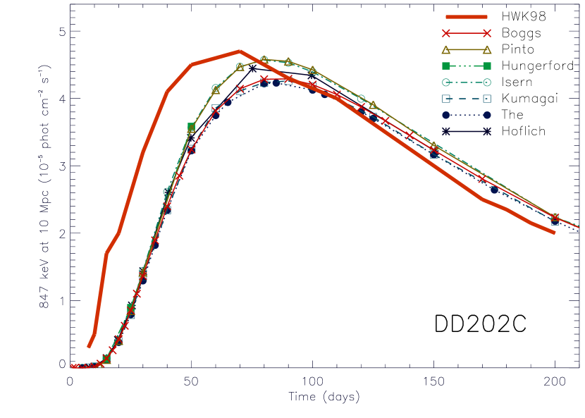
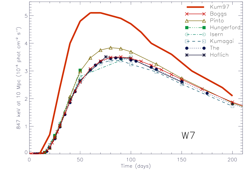
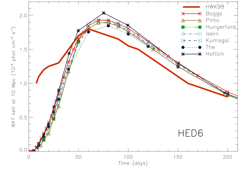
Figure 10: Line fluxes of the 847 keV line for the SN models, DD202C (upper panel), W7 (middle panel) and HED6 (lower panel). Spectral extraction was more complicated for the 847 keV line than for the 1238 keV line (requiring the assumption that the 847 & 812 escape fractions are equal, and that all emission in the 790 - 900 keV energy band is line emission), but the light curves agree well with the light curves that result from tagging photons. Again, all current simulations suggest less line emission than suggested in HWK98 & Kumagai 1997. Also, the scaling for escape fraction and branching ratios brings the HWK98 light curves into rough agreement with the other light curves.

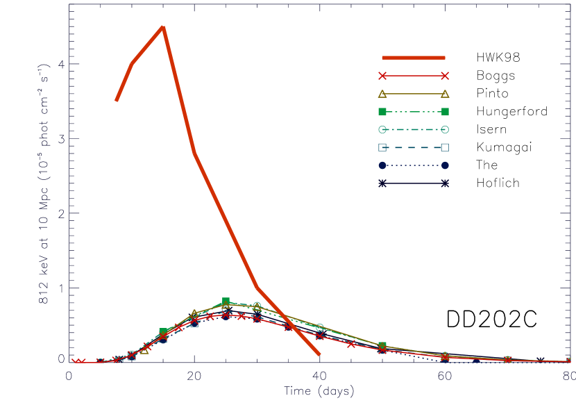
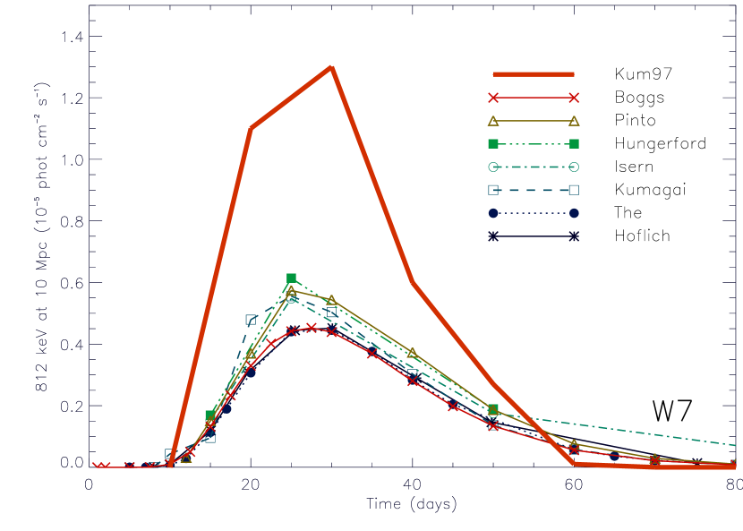
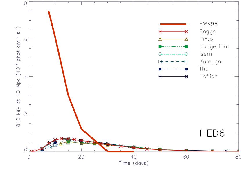
Figure 11: Line fluxes of the 812 keV line for the SN models, DD202C (upper panel), W7 (middle panel) and HED6 (lower panel). As with the 812 keV line emission, the spectral extraction and tagging light curves agree, and are fainter than the HWK98 & Kumagai 1997 light curves. With the scaling for escape fraction and branching ratios, the HWK98 light curves agree fairly well with the other light curves. The HWK98 light curves after 20-30 days fall to zero, faster than the other light curves; this is due to the different definition for the 812 keV line employed in that work.

In Figures 10 and 11, we show the 847 keV and 812 keV line fluxes for the three models as simulated by all seven codes. Again for comparison, we include earlier light curves from HWK98 and Kumagai & Nomoto (1997). The deviation at late times ($>25$ days) for the HWK98 812 keV light curve is consistent with the lower adopted branching ratio used in that code (see $\S$2.2.1). As with the 1238 keV light curves, we find the same good agreement between the current code results.

3.4 Summary of Comparisons

In light of the previous differences in simulated SN Ia gamma-ray spectra, the agreement demonstrated in this comparison is strongly encouraging. The differences between the individual simulations are generally at the 10-20% level, much less than the differences that result from a range of input explosion models. This is particularly apparent in the nine panels of Figures 7 and 8. There would be no ambiguity as to which is the correct scenario if these three models were compared with actual observations of sufficient sensitivity. While it is true that very similar models might be unresolvable due to the current variations between simulations, the level of accuracy required to perform this type of observation will not be realized in the forseeable future.

Since we have chosen a set of explosion models that probably represent the full range of SNe Ia explosions, these models provide an ideal testing ground for gamma-ray transport codes and it is likely that codes that get good agreement against the spectra and light curves presented here can be trusted using different explosion models as well.

Having demonstrated that the simulations have converged upon similar solutions for these three models, we explore the range of SN Ia events considered possible ($\S$4) and compare these simulations with observations ($\S$5).

4 SN Ia Line Fluxes

With the current agreement of all seven codes for a range of explosion models, we can now use the simulated gamma-ray signal to predict observational differences between the explosion models. Over the next few years, the challenge in gamma-ray observations will be to make a detection of a single, time-averaged flux (requiring a lengthy exposure). The dominant, 847 keV line flux peaks 50 or more days after the SN explosion, so there is ample time for the SN to be detected and identified through optical observations before gamma-ray observations must commence. The 812 keV line evolves on a shorter timescale (10-35d) and has a fainter peak (limiting its detection to very local supernovae). As the SN takes roughly the same timescale to reach the optical peak, gamma-ray observations need to commence a few days before optical peak to contain the 812 keV peak. A large fraction of nearby SNe Ia are detected at peak or later, so this requirement places strict demands upon “target-of-opportunity” telescopes.

In this section we show line flux light curves for a collection of SN Ia models simulated with the The code. We separate the models into three sub-classes based on observational categories: normally-luminous, sub-luminous and super-luminous.

4.1 Normally-luminous SNe Ia

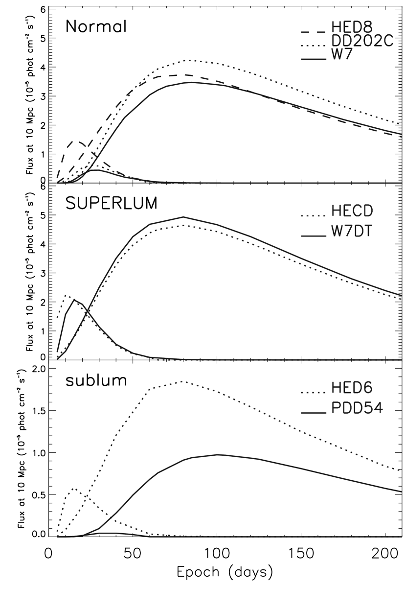
Figure 12: Line fluxes of the 812 & 847 keV lines for SN models representative of the 3 luminosity sub-classes. The super-luminous models (W7DT & HECD) have the brightest gamma-ray lines, but are the most homogeneous, while the sub-luminous models (PDD54 & HED6) are faint but differ appreciably. The Chandrasekhar-mass normally-luminous models (W7 & DD202C) differ at late times due to their different nickel production, and the sub-Chandrasekhar mass model (HED8), differs early due to nickel produced very near the surface.

This is the most frequent SN Ia sub-class and the best studied. SN 1998bu was considered normally-luminous and is grouped in this category (§5.3). We compare three models that fit within this sub-class, W7 (a Chandrasekhar-mass deflagration); DD202C (a Chandrasekhar-mass delayed detonation) and HED8 (a sub-Chandrasekhar mass helium detonation). The light curves are shown in the upper panel of Figure 12. HED8 creates the least amount of nickel, but has nickel near the surface. This leads to HED8 being the brightest model of the three at early epochs, but the faintest model after 150 days. For a sufficiently early observation of a nearby supernova, DD202C and W7 are easily distinguished from HED8 based upon the 812 keV line (or equivalently, the timing of the rise of the 847 keV line).

4.2 Super-luminous SNe Ia

This SN Ia sub-class differs from the normally-luminous SNe Ia in that the explosion creates more nickel for each scenario. SN 1991T was considered super-luminous and is grouped in this sub-class (§5.2). We compare two models, W7DT (a Chandrasekhar-mass late detonation that is very similar to W7 but includes additional nickel production nearer the surface) and HECD (a sub-Chandrasekhar mass helium detonation that is more massive and produces more nickel that HED8). These models produce brighter light curves (middle panel of Figure 12), but the two super-luminous explosion models do not differ dramatically, and it will be difficult to distinguish them based on the gamma-ray light curves alone. The result is that this type of explosion is detectable to large distances, but is not distinguishable to a comparatively large distance.

The super-luminous models are characterized by nickel near the surface of the ejecta. While this leads to 812 keV emission at earlier epochs than predicted for normally-luminous SN Ia models, the 812 keV peak is much lower than suggested in HWK98 and Kumagai & Nomoto (1997). The largest deviations between past works and this current work occur in this “super-luminous” type Ia subclass.

4.3 Sub-luminous SNe Ia

This sub-class is the least promising for gamma-ray studies. SN 1986G was considered a slightly sub-luminous event and is best (though imperfectly) grouped in this sub-class (§5.1). Sub-luminous events are less frequent than normally-luminous SNe Ia and produce much fainter gamma-ray emission. For Chandrasekhar-mass explosions, the nickel production is very low and is all concentrated near the center of the supernova. This results in extremely faint gamma-ray emission. Sub-Chandrasekhar mass explosions also produce very little nickel, but occur in lower mass objects, so the high escape fractions partially compensate for the lower nickel production. We compare two models, PDD54 (a Chandrasekhar-mass pulsed delayed detonation) and HED6 (a very low-mass helium detonation). Different Sub-luminous models produce quite different light curves, but all are so faint that they will be difficult to detect (lower panel of Figure 12).

5 Observed SNe Ia

In the last 25 years, there have been three SNe Ia that were close enough to warrant observations with gamma-ray telescopes. Although none of the three resulted in significant detections, papers have been written that infer the nickel production in each SN based upon the observations. We revisit these three observations and discuss to what level they constrain the potential explosion mechanisms.

5.1 SMM Observations of SN 1986G

SN 1986G was first detected in Centaurus A on May 3, 1986 (Evans 1986, IAU Circ., No. 4280). It was discovered one week before maximum light and exhibited a relatively narrow luminosity peak. Its high $\Delta$m₁₅(B) value led to its classification as a slightly sub-luminous SN (Hamuy et al. 1996). Heavy host galaxy extinction was suggested by both the photometric colors and by strong Na-D absorption. Although some papers have argued that the extinction was large enough to infer an absolute magnitude in the normal range (Cristiani et al. 1994), recent studies of the host galaxy extinction to SNe Ia maintain that SN 1986G was slightly sub-luminous (Phillips et al. 1999).

The Gamma-Ray Spectrometer on-board the Solar Maximum Mission (SMM) satellite observed the SN with sensitivity that varied from 30% to full sensitivity during the entire epoch of cobalt decay. Matz & Share (1990) derived upper limits for the 847 and 1238 keV line emission from SMM spectra. They used escape fractions published by Gehrels, Leventhal & MacCallum (1987) from a collection of parameterized SN Ia models to derive that the upper limits for the nickel production ranged from 0.36 - 0.41 M_⊙ (assuming a distance of 3 Mpc to Centaurus A). This upper limit is marginally consistent with the 0.45 $\pm$ 0.03 M_⊙ ⁵⁶Ni production (scaling the distance from 3.3 $\pm$ 0.3 Mpc to 3.0 Mpc) derived from the nebular spectra (Ruiz-Lapuente & Lucy 1992).

Matz & Share quoted their results in terms of the ⁵⁶Ni production allowed by the observations. We do not re-analyze the SMM observations. Instead, we compare the average fluxes during the 1986 August 25 - October 9 interval during which the SMM sensitivity was the largest. A review of the escape fractions from Gehrels, Leventhal & MacCallum (1987) confirms that their range is in agreement with the simulations performed in this work. The SMM instrument had a $\sim$ 80 keV FWHM at these energies and thus sampled a broad range of the continuum in addition to the two lines. However, for most of the epochs included in the composite SMM observation, the SN would have been expected to emit a relatively faint continuum. Thus, very little error is introduced by using tagged line photons and ignoring the instrument energy resolution for this SN.

In Figure 13, we compare light curves for five models with the light curves for the three models treated in Matz & Share, in all cases setting the distance to be 3.3 Mpc. The three Matz & Share light curves assume the 3$\sigma$ upper limit ⁵⁶Ni masses, the other models use the published masses (as listed in Table 3). While only the 847 keV line emission is shown in the figure, the upper limit ⁵⁶Ni masses were based upon a joint 847-1238 keV line fit. The figure shows that the three normally-luminous SN Ia models (DD202C, W7 and HED8) all produce too much 847 keV emission, while the very sub-luminous SN Ia models are faint enough to remain below the upper limits, especially for the low-nickel PDD54.

Note that all of these light curves assume the distance to Centaurus A to be 3.3 Mpc. Measures of this distance arrive at 3.1 $\pm$ 0.1 Mpc (Tonry & Schecter 1990) and 3.6 $\pm$ 0.2 Mpc (Jacoby et al. 1988), suggesting that slightly more ⁵⁶Ni production could be permissible. Thus, it appears that SN 1986G was tantalizingly close to being detected by SMM, and it would have been detected had it been a normally- or super-luminous event rather than slightly sub-luminous. Nonetheless, the upper limit is consistent with the current understanding of SNe Ia and the simulation of gamma-ray escape from SN models.

5.2 CGRO/COMPTEL and OSSE of SN 1991T

SN 1991T was first detected in NGC 4527 on April 13, 1991 (S. Knight, IAU Circ., No. 5239) more than a week before maximum light. Its pre-maximum spectra featured iron-peak elements instead of the intermediate-mass elements of normal SNe Ia supernovae, but, after peak, it was spectro-scopically normal. The light curves were broad ($\Delta$m₁₅(B) value of 0.94), leading to the suggestion that SN 1991T was a super-luminous SN Ia and it became a template slow SN Ia (though slower SNe exist). SN Ia models were produced explicitly to explain the optical observations of 1991T, we have included two of these models in this study (W7DT and HECD).

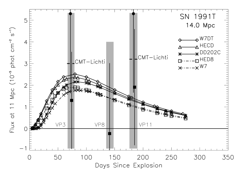
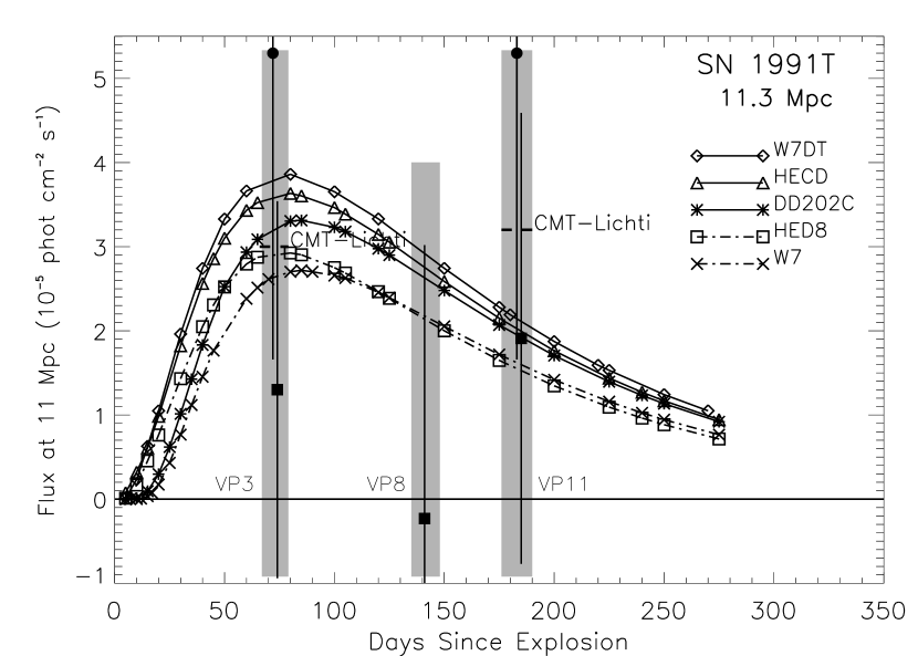
Figure 14: Five current simulations of 847 keV line emission from SN Ia models at two assumed distances are compared with COMPTEL and OSSE observations of SN 1991T. The upper panel shows the models at the larger distance of 14.0 Mpc, the lower panel shows the models at 11.3 Mpc. The five current simulations are identified as shown. The shaded regions show the three viewing periods, VP3, VP8 (OSSE-only) and VP11. The OSSE data points (filled boxes) and COMPTEL-Lichti (2$\sigma$ upper limits, dashed lines) are fainter than the models, while the COMPTEL-Morris (filled circles) are brighter than the models (Lichti et al. 1994, Leising et al. 1995, Morris et al. 1997). The fluxes were all derived from joint 847/1238 keV line fits.

The Compton Gamma-Ray Observatory had just been launched (one week before the discovery of SN 1991T), and months of calibrations and other testing had to be performed before the instruments on-board CGRO could observe the SN. Observations were initiated on June 15, 67 days after the explosion (assuming the SN was detected 3 days after the explosion), and continued in three viewing periods (3,8,11) until 190 days after the explosion (COMPTEL observed only viewing periods 3 and 11). There were two instruments on CGRO that were capable of detecting the 847 and 1238 keV lines from the SN, the COMPTEL and OSSE instruments. Separate analyses were performed upon the two sets of observations. Initially, COMPTEL reported only upper limits for the 847 and 1238 keV lines, arriving at 2$\sigma$ upper limits for the 847 keV line of 3.0 x 10^-5 phot $cm^{-2}$ $s^{-1}$ and 3.2 x 10^-5 phot $cm^{-2}$ $s^{-1}$ for each viewing period (Lichti et al. 1994). A later, independent analysis suggested a combined 3.3$\sigma$ detection (Morris et al. 1997). OSSE analysis derived only upper limits, reporting a 3$\sigma$ upper limit of (4.1-6.6) x 10^-5 phot $cm^{-2}$ $s^{-1}$ for the 847 keV line during the first observation, based upon a combined, simulataneous fit to the 847 keV and 1238 keV lines during all three epochs (Leising et al. 1995). When fit separately, the formal fluxes are (1.3$\pm$2.2, -0.2$\pm$3.2, 1.9$\pm$2.7) x 10^-5 phot $cm^{-2}$ $s^{-1}$ for the 847 keV line for each of the three viewing periods (M.D. Leising, personal communication). We compare five models to the OSSE observations combined with each of the COMPTEL results (Figure 14).

The uncertainty of the distance to NGC 4527 has made interpretation of the upper limits to the gamma-ray emission complicated. Using the distances to suggested neighbor-galaxies yielded a range of distances from 10-17 Mpc. With such a range, astronomers could either largely reject the Ia models by the observed upper limits or find that almost all models were consistent. (see Leising et al. 1995 for an explanation of the difficulties simultaneously explaining the optical and gamma-ray observations of SN 1991T). New studies have narrowed the distances to a range from 11.3-14.0 Mpc (Richtler et al. 2001, Gibson & Stetson 2001, Saha et al. 2001). For this work, we place NGC 4527 at 11.3 and 14.0 Mpc.

OSSE did not detect emission from SN 1991T, although VP3 was very near the peak of the simulated cobalt line peaks. Thus, those observations favor models that feature low gamma-ray fluxes. However, the modest sensitivity of the OSSE instrument limits the ability to discriminate between explosion scenarios.

The COMPTEL observations would, in principle, strengthen the ability to distinguish explosion scenarios. However, this is not (unambiguously) the case because the two separate analyses of the COMPTEL data arrived at dramatically different conclusions. The analysis by Lichti et al. (1994) detected no emission from SN 1991T, and thus favors models that feature low gamma-ray fluxes. When combined with the OSSE observations, the COMPTEL upper limits further favor low gamma-ray flux models, at the level that the brighter models would be considered inconsistent (Leising et al. 1995). By constrast, the Morris et al. (1997) analysis measures fluxes brighter than predicted by any of the models. Using those fluxes, the highest flux models are favored, the more sensitive COMPTEL observations counteracting the OSSE upper limits.

The inability to reconcile these datasets severely limits the physics that can be derived from the observations (at least at the current level of understanding of SN Ia explosion physics). The OSSE observations do not reject any of the explosion scenarios if the larger NGC 4527 distance is used, and the COMPTEL observations are ambiguous.

5.3 CGRO/COMPTEL Observations of SN 1998bu

SN 1998bu was discovered by M. Villi on May 9, 1998 (IAU Circ., No. 6899) in M96 (NGC 3368) more than a week before maximum light, affording CGRO a second opportunity to observe a SN Ia. This SN was determined to be a normally-luminous SN ( $\Delta$m₁₅(B) = 1.02 $\pm$ 0.04, Jha et al. 1999). Distance estimates have ranged from 9.6$\pm$0.6 Mpc from planetary nebulae (Feldmeier et al. 1997) to 11.6$\pm$0.9 Mpc from HST-Cepheid period luminosity estimates (Tanvir et al. 1995). Subsequent HST-Cepheid period luminosity estimates place M96 at 9.9 - 11.3 Mpc (Gibson & Stetson 2001, Gibson et al. 2000, Hjorth & Tanvir 1997), the range we will use in this study. The CGRO team was able to begin observations at about maximum light. A total of 88 days of observing by both the COMPTEL and the OSSE instruments were devoted to SN 1998bu (spanning 17-136 days after the explosion), again resulting in two separate data-sets. Neither instrument detected 847 or 1238 keV line emission. The OSSE instrument reported a 3$\sigma$ upper limit for 3 x 10^-5 phot cm^-2 s^-1 for the 847 keV line based upon a combined fit to the 847 keV and 1238 keV lines (Leising at el. 1999). When treated separately, the derived formal fluxes are (1.2$\pm$1.4) x 10^-5 phot cm^-2 s^-1 and (-0.6 $\pm$1.6) x 10^-5 phot cm^-2 s^-1 for the 847 keV and 1238 keV lines (M.D. Leising, personal communication). The COMPTEL 2$\sigma$ upper limits are 3.1 x 10^-5 phot cm^-2 s^-1 and 2.3 x 10^-5 phot cm^-2 s^-1 respectively (using the lower of the imaging and spectral analysis results for each line, from Georgii et al. 2002).

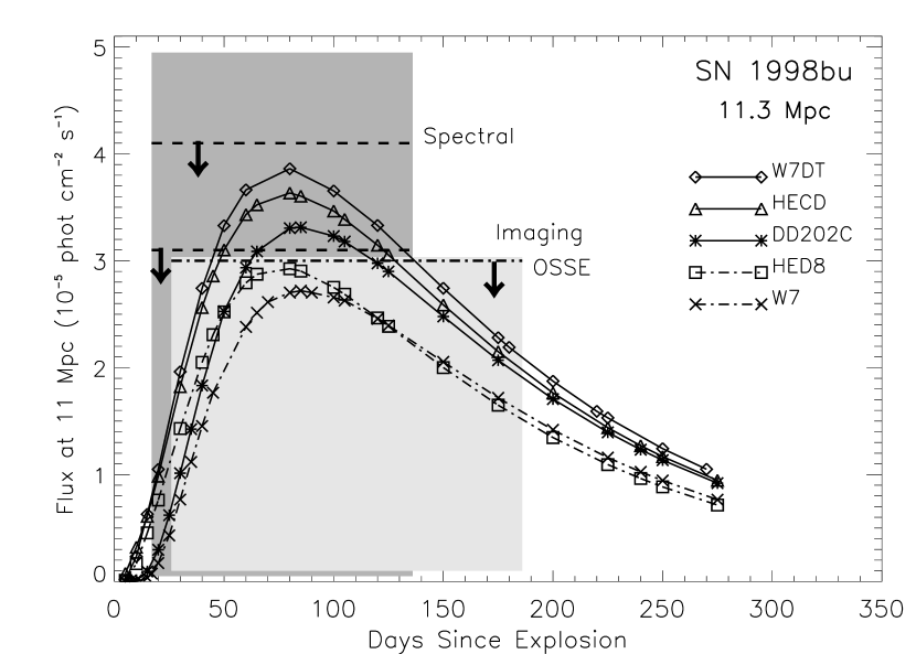
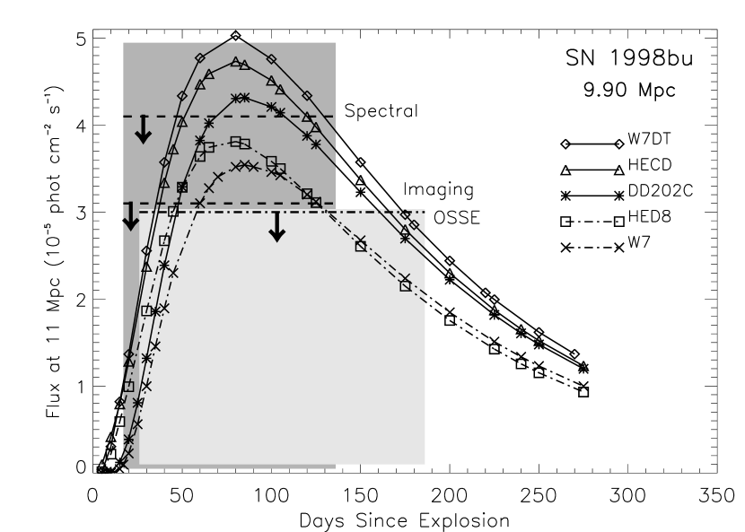
Figure 15: Five current simulations of 847 keV line emission from SN Ia models at two assumed distances are compared with COMPTEL and OSSE observations of SN 1998bu. The upper panel shows the models at the larger distance, 11.3 Mpc, the lower panel shows the models at 9.9 Mpc. The five current simulations are identified as shown. The light shaded region shows roughly the epoch of OSSE observations, the dark shaded region shows roughly the epoch of COMPTEL observations. The two COMPTEL upper limits (Imaging and Spectral, dashed lines) are at the 2$\sigma$ level (Georgii et al. 2001). The OSSE 3$\sigma$ upper limits (dot-dashed line) are based upon a joint 847/1238 keV line fit. Table 4 shows the probabilities of each model being consistent with the data at the two distances.

We first study the larger distance to NGC 3368. Comparison of the three normally-luminous SN models with these upper limits finds that W7 and HED8 peak at or below the COMPTEL imaging upper limit for the 847 keV line, and that average flux of DD202C is approximately equal to the COMPTEL imaging upper limit (Figure 15). All three models are consistent with the combined OSSE and COMPTEL, 847 keV and 1238 keV data at a 10% probability, or better using the chi-squared test to the individual data points (Table 4). The super-luminous SN models (HECD and W7DT) are brighter than the normally-luminous models, and are less likely to be as faint as the combined measurements. Considering that the optical observations favor a normally-luminous SN Ia, the non-detection is consistent with expectations.

Assuming the shorter distance to NGC 3368, the upper limits become a great deal more constraining. Only W7 appears to be faint enough to rise above the 2% probability level for having neither instrument detect emission from the SN. The gamma-ray observations appear to favor a larger distance to NGC 3368.

Comparing these interpretations with Georgii et al. 2002, the conclusions are similar, but not identical. Principally, at the larger distance, that work only rejects the high-⁵⁶Ni producing models, while at the shorter distance that work rejects all normally-luminous models. They use the light curves shown in Kumagai & Nomoto 1997, for HECD, W7DT, W7 and WDD2, which were high as discussed in $\S 4$. The delayed detonation light curves from that work are very similar to the DD202C light curve shown in Figure 15. We note that Table 1 in that work shows average fluxes that correspond to their shorter distance of 9.6 Mpc, not the 11.3 Mpc shown in their Figure 6, and should thus be compared with our column 1 in Table 4. It is also worth noting that the CGRO observations spanned the epoch at which normally-luminous models predict the brightest 847 and 1238 keV line emission. Thus, the non-detection is not likely to have been affected by delay in the CGRO observations.

6 Conclusions

In this paper, we compare gamma-ray emission simulations from 7 transport codes using a diverse set of SNe Ia models. The spectra for 3 models (DD202C, W7, HED6) at explosion times ranging from 5 to over 200 days provide tests of these codes for a range of extreme conditions. This information allowed us to track down a number of errors in past results and correct for these errors. The results of HWK98 and Kumagai & Nomoto (1997) had the most dramatic errors, but their revised “current” codes now agree much better with our “unified” solution.

To the extent that 1D SN Ia models closely approximate the physical SN explosion, observations can now be confidently compared with simulations. With current explosion scenarios and precise flux measurements, sub-Chandrasekhar mass models can be clearly distinguishable from Chandrasekhar mass models for normal and sub-luminous SNe Ia. However, with a suitably sensitive instrument, comparisons between line shapes, in addition to line fluxes, provide the best means to distinguish different explosion scenarios (HWK98).

Contrary to some of the past results, comparing to current data on SNe Ia finds that, for the sub-class of each explosion, theoretical gamma-ray line fluxes from 1D models are consistent with the observations. However, bear in mind that the explosion scenarios shown are limited by the adequacy of 1-dimensional modeling, and truly accurate comparisons will require 3-dimensional explosions and transport calculations. In particular, clumping and global asymmetries will produce line profiles that differ from the profiles shown in this study. The wide range of line profiles possible with 3-dimensional simulations, and the resulting potential for confusion was partial motivation for this study.

Finally, recall that the inverse of calculating the gamma-rays that escape the SN ejecta (producing the gamma-ray flux) is the energy that is deposited into the SN ejecta. The ability to simulate the optical/IR/UV light curves of SNe Ia depends upon this deposition being accurately treated. This project does not directly address the energy deposition aspect of these simulations (and thus makes no claims), but errors in the decay rates and escape fraction may also lead to discrepancies in the energy deposition. Gamma-ray transport, which provides the initial input for the emission of optical light, must be understood to model the optical light curves of supernovae.

The authors would like to thank Peter Höflich for assistance in running his gamma-ray transport code, MC-GAMMA, and Mark Leising for providing OSSE results from SNe 1991T and 1998bu.

This work was performed under the auspices of the US Department of Energy by Los Alamos National Laboratory, under contract W-7405-ENG-36, and by the National Science Foundation (CAREER grant AST 95-01634), with support from DOE SciDAC grant number DE-FC02-01ER41176. L.-S. The acknowledges support from the DoE HENP Scientific Discovery through Advanced Computing Program.”

Table 1: Characteristics of Seven Gamma-ray Transport Algorithms

Simulation		Monte	Tag or	Bin Width	Line	Density	Positr.
Creator		Carlo	Spec.a	@ 847 keV	Broadb	Evolvec	Fraction
or Name	Ref.	$[y/n]$	$[T/S]$	[keV]	$[y/n]$	$[y/n]$	f(Ps)
					($\S$ 2.1.1)	($\S$ 2.1.2)	($\S$ 2.2.2)
Boggs	(1)	N	T	2.8	Y	Y	—
Pinto	(2)	Y	S	2.4	Y	Y	0.0
Höflich	(3)	Y	S	2.4	Y	N	1.0
Isern	(4)	Y	S	2.1	Y	Y	1.0
Kumagai	(5)	Y	T	50	N	N	0.0
Hungerford	(6)	Y	T	0.5	Y	N	0.0
The	(7)	Y	T	40	N	N	1.0

Simulation	Time	Source	Interactions
Creator	Dilationd	Evolvee	Treatedf
	$[y/n]$	$[y/n]$	$[CS,PE,PP]$
	($\S$ 2.2.3)	($\S$ 2.2.3)	($\S$ 2.3)
Boggs	Y	Y	CS,PE
Pinto	N	N	CS,PE,PP
Höflich	Y	N	CS,PE,PP
Isern	Y	N	CS,PE,PP
Kumagai	N	N	CS,PE,PP
Hungerford	N	N	CS,PE,PP
The	N	N	CS,PE,PP

a Is the line flux derived from determining the escape fraction of “tagged” line photons, or

extracted from the spectrum and subject to line blending and continuum contamination?

b Are the photons emitted with Doppler broadening due to the differential expansion of the ejecta?

c Does the algorithm evolve the ejecta density after the photon emission to account for

non-zero crossing times?

d Are the relativistic effects of time dilation on the decay rate included?

e Does the algorithm account for the effect of requiring simultaneous photon arrival from

the near/far side of the ejecta?

f The interactions treated are CS = Compton Scattering, PE = Photoelectric Absorption,

PP = Pair Production.

REFERENCES. (1) Boggs (ApJ submitted) ; (2) Pinto, Eastman & Rogers 2001;

(3) Höflich, Khokhlov & Wheeler 1998; (4) Isern, Gomez-Gomar,

Bravo & Jean 1997; (5) Kumagai 1996; (6) Hungerford et al. 2003;

(7) The & Burrows 1991.

Table 2: Important Gamma-ray Line for ⁵⁶Ni and ⁵⁶Co Decays. Lines studied in this work are listed in bold font. All ratios are from the 8th Table of Isotopes (1996).

56Ni Decay		56Co Decay
Energy	Intensity	Energy	Intensity
$[keV]$	$[phot/100decays]$	$[keV]$	$[phot/100decays]$
158	98.8	847	100
270	36.5	1038	14
480	36.5	1238	67
750	49.5	1772	15.5
812	86.0	2599	16.7
1562	14.0	3240a	12.5

a This line is the sum of a three line complex.

Source	Reference	$\tau$(Ni56)	$\tau$(Co56)
of Half-lives	and Year	[d]	[d]
Nuc. Data Sheets	Junde 1999	6.075	77.233
Table of Isotopes(8th)	Firestone 1996	5.9	77.27
Table of Rad. Isotopes	Browne & Firestone 1986	6.10	77.7
Table of Isotopes(7th)	Browne & Dairiki 1978	6.10	78.8
Table of Isotopes(6th)	Lederer & Shirley 1967	6.1	77

Table 3: Characteristics of SN Ia Explosion Models

Model	Mode of		M∗	MNi	Ekin
Name	Explosion	Ref.	(M⊙)	(M⊙)	(1051 ergs s-1)
Algorithm Comparison
DD202C	Delayed det.	(1)	1.40	0.72	1.33
HED6	He-det.	(2)	0.77	0.26	0.74
W7	Deflagration	(3)	1.37	0.58	1.24
Spanning Explosions
PDD54	Pul.del.det.	(4)	1.40	0.14	0.35
W7DT	Late det.	(5)	1.37	0.76	1.61
HED8	He-det.	(2)	0.96	0.51	1.00
HECD	He-det.	(6)	1.07	0.72	1.35

REFERENCES. (1) Höflich et al. 1998; (2) Höflich & Khokhlov 1996;

(3) Nomoto et al. 1984; (4) Höflich, Khokhlov & Wheeler 1995; (5) Yamaoka

et al. 1992; (6) Kumagai 1997.

Table 4: Comparisons of SN Ia models with SN 1998bu

SN 1998bua
Model	$F_{10Mpc}^{75days}$	Consistency at 9.9 Mpc	Consistency at 11.3 Mpc
Name	[$10^{-5}cm^{-2}s^{-1}$]	[%]	[%]
W7	3.3	3.87	29.4
HED8	3.7	1.48	19.8
DD202C	4.1	0.40	11.5
W7DT	4.6	0.05	4.73
HECD	4.9	0.02	2.84

a OSSE data from Leising et al. 1999, COMPTEL data from Georgii et al. 2002.

Figure 2: Line shifting due to the expansion of the ejecta of four SN models. The fractional line shift due to the expansion of the ejecta is plotted on the left axis, the shift for the 847 keV line is shown on the right. For reference, ⁵⁶Ni-rich regions of the ejecta are shown in the upper left as thick, horizontal bars.

References

- (1) Ait-Ouamer, A.D. et al. 1990, in Proceedings of the 21st International Cosmic Ray Conference, University of Adelaide Press, Vol. 2, 183
- (2) Ajhar, E.A., Tonry, J.L., Blakeslee, J.P., Riess, A.G., Schmidt, B.P. 2001, ApJ, 559, 584
- (3) Ambwani, K., & Sutherlan, P. 1988, ApJ, 325, 820
- (4) Boggs, S.E., & Jean, P. 2001, A&A, 376, 1126
- (5) Browne, E., Dairiki, J.M., & Doebler, R.E. 1978, Table of Radioactive Isotopes, Eds. C.M. Lederer, & V.S. Shirley, John Wiley & Sons, p. 160
- (6) Browne, E. & Firestone, R.B. 1986, Table of Radioactive Isotopes, Ed. V.S. Shirley, John Wiley & Sons, p. 56-2
- (7) Brown, B.L., & Leventhal, M. 1987, ApJ, 319, 637
- (8) Burrows, A. & The, L.-S. 1990, ApJ, 360, 626
- (9) Bussard, R.W., Burrows, A., The, L.-S. 1989, ApJ, 341, 401
- (10) Chan, K.-W., & Lingenfelter, R.E. 1989, ApJ, 318, L51
- (11) Chan, K.-W., & Lingenfelter, R.E. 1993, ApJ, 405, 614
- (12) Clayton, D.D., Colgate, S.A., Fishman,G.J. 1969, ApJ, 155, 75
- (13) Clayton, D.D., & The, L.-S. 1991, ApJ, 375, 221
- (14) Cristiani, S. et al. 1992, A&A, 259, 63
- (15) Evans, R. 1986, IAU Circular, 4208
- (16) Firestone, R.B. 1996, 8th Table of Isotopes, Ed. V.S. Shirley, John Wiley & Sons, p. 249
- (17) Friedman, W.L. et al. 2001, ApJ, 553, 47
- (18) Gibson, B., & Stetson, P.B. 2001, ApJ, 547, L103
- (19) Gibson, B. et al. 2000, ApJ, 529, 723
- (20) Gehrels, N., Leventhal, M., MacCallum, C.J. 1987, ApJ, 322, 215
- (21) Georgii, R. et al. 2002, A&A, 394, 517
- (22) Gómez-Gomar, J.,Isern, J., & Jean, P. 1998, MNRAS, 295, 1
- (23) Hamuy, M., et al. 1996, AJ, 112, 2391
- (24) Harris, M. et al. 1998, ApJ, 501, L55
- (25) Harrison, F.A., et al. 2003, SPIE, 4851, 345
- (26) Hjorth, J., & Tanvir, N.R. 1977, ApJ, 482, 68
- (27) Höflich, P., Khokhlov, A., Müller, E. 1992, A&A, 259, 549
- (28) Höflich, P., & Khokhlov, A. 1996, ApJ, 457, 500
- (29) Höflich, P., Wheeler, J. C., & Khokhlov, A. 1998, ApJ, 492, 228
- (30) Höflich, P., Wheeler, J. C., & Thielemann, F.-K. 1998, ApJ, 495, 617
- (31) Höflich, P. 2002, New Astronomy Reviews, 46, 475
- (32) Hungerford, A.L., Fryer, C.L., Warren, M.S. 2003, ApJ, 594, 390
- (33) Isern, J., Gómez-Gomar, J., & Bravo, E. 1996, Memorie della Societa Astronomia Italiana, 67, 101
- (34) Isern, J., Gómez-Gomar, J., Bravo, E., & Jean, P. 1996, in Proceedings of the 2nd INTEGRAL Workshop, Eds. C. Winkler, J.-L. Courvoisier, Ph. Drouchoux, ESA, p. 89
- (35) Iwabuchi, K. & Kumagai S. 2001, PASJ, 53, 669
- (36) Jacoby, G.H., Ciardullo, R., Ford, H.C. 1988, The Extragalactic Distance Scale, Provo: BYU Press, p. 42
- (37) Jha, S. et al. 1999, ApJS, 125, 73
- (38) Junde, H. 1999, Nucl. Data Sheets, 86, 315
- (39) Kazaryan, S.M. et al. 1990, in Proceedings of the 21st International Cosmic Ray Conference, University of Adelaide Press, Vol. 2, 187
- (40) Kinzer, R.L. et al. 2001, ApJ, 559, 282
- (41) Kumagai, S., & Nomoto, K. 1997, in Proceedings of the NATO ASI on Thermonuclear SNe (C486), eds. P. Ruiz-Lapuente,R. Canal, & J. Isern, Kluwer, Dordrecht, p. 515
- (42) Kumagai, S., Iwabuchi, K., & Nomoto, K. 1999, in Proceedings of Astronomy with Radioactivties III (MPE Report 274), eds. R. Diehl & D. Hartmann, Max-Planck Institute for Extra-terrestrial Physics, p. 181
- (43) Kurfess, J.D. et al. 1992, ApJ, 399, L141
- (44) Lederer, C.M., Hollander, J.M., & Perlman, I. 1967, 6th Table of Isotopes, John Wiley & Sons, p. 189
- (45) Leising, M.D. et al. 1995, ApJ, 450, 805
- (46) Leising, M.D., The, L.-S., Höflich, P., Kurfess, J.D., Matz, S. 1999, BAAS-HEAD, 31, 703
- (47) Li, W.D., Filippenko, A.V., Riess, A.G., Treffers, R.R., Hu, J.Y., & Qui, Y.L. 2000, in Cosmic Explosions, AIP Proceedings 522, eds. S.S. Holt & W.W. Zhang, p. 91
- (48) Lichti, G.G. et al. 1994, A&A, 292, 569
- (49) Livio, M. 2001, in Greatest Explosions Since the Big Bang, Cambridge University Press, eds. M. Livio, N. Panagia, & K. Sahu, p. 334
- (50) Mahoney, W.A. et al. 1988, ApJ, 334, L81
- (51) Matz, S.M. & Share, G.H. 1990, ApJ, 362, 235
- (52) Milne, P.A., The, L.-S., & Kroeger, D. 2000, in Proceedings of the 2nd Chicago Meeting on Thermonuclear Explosions, ed. J. Niemeyer, in press
- (53) Milne, P.A., Kroeger, D., Kurfess, J.D., & The, L.-S. 2002, New Astronomy Reviews, 46, 617
- (54) Mochizuki, Y., Takahashi, K., Janka H.-TH., Hillebrandt, W., Diehl, R. 1999, A&AS, 346, 831
- (55) Morris, D.J., Bennett, K., Bloemen, H., et al. 1997, Proc. of the 4th Compton Symp., AIP Conf. Proc., 410, 1084
- (56) Müller, E., Höflich, P. & Khokhlov, A. 1991, A&A, 249, L1
- (57) Nomoto, K., Thielemann, F.-K., & Yokoi, K. 1984, ApJ, 286, 644
- (58) Ore, A., & Powell, J. 1949, Phys. Rev., 75, 1696
- (59) Pinto, P.A., & Woosley, S. 1988, Nature, 333, 534
- (60) Pinto, P.A., & Eastman, R. 2000, ApJ, 530, 744 (2000a)
- (61) Pinto, P.A., & Eastman, R. 2000, ApJ, 530, 757 (2000b)
- (62) Pinto, P.A., Eastman, R., Rogers, T. 2001, ApJ, 551, 231
- (63) Perlmutter, S. et al. 1999, ApJ, 483, 565
- (64) Phillips, M.M., Lira, P., Suntzeff, N.B., Schommer, R.A., Hamuy, M., & Maza, J. 1999, AJ, 118, 1766
- (65) Rester, A.C. et al. 1989, ApJ, 342, L71
- (66) Richtler, T., Jensen, J.B., Tonry, J., Barris, B., Drenkhahn, G. 2001, A&A, 368, 391
- (67) Riess, A.G. et al. 1998, AJ, 116, 1009
- (68) Ruiz-Lapuente, & P., Lucy, L.B. 1992,ApJ,400,127
- (69) Saha, A. et al. 2001, ApJ, 551, 973
- (70) Shigeyama, T., Kumagai S., Yamaoka, H., Nomoto, K., Thielemann, F.-K. 1993, A&AS, 97, 223
- (71) Tanvir, N.R., Shanks, T., Ferguson, H.C., Robinson, D.R.T. 1995, Nature, 377, 27
- (72) Teegarden, B.J., Barthelmy, S.D., Gehrels, N., Tueller, J., Leventhal, M. 1989, Nature, 339, 122
- (73) The, L.-S., Burrows, A., & Bussard, R. 1990, ApJ, 352, 731
- (74) The, L.-S., Leising, M.D., & Clayton, D.D. 1993, ApJ, 403, 32
- (75) The, L.-S., Bridgeman, W., & Clayton, D.D. 1994, ApJS, 93, 531
- (76) Tonry, J.L., & Schechter, P.L. 1990, AJ, 100, 1794
- (77) Tueller, J. et al. 1990, ApJ, 351, L41
- (78) Villi, M. 1998, IAU Circ., 6899, 000