Fe II and Mg II in Luminous, Intermediate-Redshift Narrow-line Seyfert 1 Galaxies from the Sloan Digital Sky Survey

Abstract

We present results from analysis of spectra from a sample of $\sim 900$ quasars from the Sloan Digital Sky Survey. These objects were selected for their intermediate redshift ($1.2<z<1.8$), placing Mg II and UV Fe II in the optical band pass, relatively narrow Mg II lines, and moderately good signal-to-noise-ratio spectra. Using a maximum likelihood analysis, we discovered that there is a significant dispersion in the Fe II/Mg II ratios in the sample. Using simulations, we demonstrate that this range, and corresponding correlation between Fe II equivalent width and Fe II/Mg II ratio, are primarily a consequence of a larger dispersion of Fe II equivalent width (EW) relative to Mg II EW. This larger dispersion in Fe II EW could be a consequence of a range in iron abundance, or in a range of Fe II excitation. The latter possibility is supported by evidence that objects with weak (zero) C II] $\lambda 2325$ equivalent width are likely to have large Fe II/Mg II ratios. We discuss physical effects that could produce a range of Fe II/Mg II ratio.

1 Introduction

The properties of UV Fe II and Mg II in Active Galactic Nuclei (AGN) are important for several reasons. Luminous quasars are probes of the early Universe. As discussed by Hamann & Ferland (1993) and others, the production of iron is thought to lag that of the $\alpha$ elements, including magnesium, due to different formation mechanisms: magnesium and about half of the iron (Nomoto, Nakamura, Kobashi, 1992) are produced in supernovae from massive, rapidly-evolving stars, while the remainder of the iron is produced largely in Type 1a supernova which involve accretion onto a white dwarf star, a process which requires approximately 1 billion years. Observation of an evolution of [Fe/Mg] with redshift could constrain the time of the first burst of star formation in the Universe. The UV Fe II and Mg II line emission are found conveniently near one another in the rest-UV bandpass, and their atomic properties are sufficiently similar that they should be strongly emitted from gas under similar physical conditions. Therefore it was thought that the Fe II/Mg II ratio could be an abundance diagnostic. No clear evidence for Fe II/Mg II ratio evolution has been observed yet (e.g., Dietrich et al., 2003). Thus, the first star formation occurred very early; alternatively, massive amounts of iron may have been produced in the first very massive stars (Heger & Woosley, 2002).

The study of Fe II is also relevant for understanding Narrow-line Seyfert 1 galaxies (NLS1s). One of the criteria used to identify NLS1s, along with their narrow H$\beta$ and weak forbidden lines, is their frequently-strong optical Fe II emission (Osterbrock & Pogge, 1985; Goodrich, 1989). NLS1s lie at one end of the Boroson & Green (1992) Eigenvector 1, and the strength of optical Fe II is a primary participant in that eigenvector. Also, we are encouraged to use NLS1s to study Fe II for pragmatic reasons. The numerous Fe II emission lines form a pseudocontinuum, but since the Fe II line widths are correlated with the H$\beta$ widths (e.g., Boroson & Green, 1992), the characteristic shape of the pseudocontinuum and even emission from individual multiplets can be identified in spectra from objects with narrow H$\beta$ lines. In broad-line objects, the Fe II is smeared, making it more difficult to study.

Understanding Fe II could be quite important for understanding AGN broad-line region (BLR) emission in general. Fe II comprises up to one third of the line emission, so it is an important coolant (Joly, 1993). The Fe⁺ ion is sufficiently complicated that it can potentially be a diagnostic of density, column density, turbulence, temperature, and continuum shape. But at the same time, Fe II emission is difficult to understand because it is so complicated, and although sophisticated models are under development (Verner et al., 1999; Sigut & Pradhan, 2003; Verner et al., 2003), none fully account for the required complex atom, ionization balance and radiative transfer.

The problem of Fe II emission in AGN spectra has been around for more than 25 years. Interest in this complicated problem has recently increased, stimulated by the availability of high signal-to-noise ratio IR spectra, the potential for determining the epoch of the first star formation, and sufficient computing power for appropriately complex models. In this paper we present some of the results of a study of the properties of UV Fe II and Mg II in a large sample of intermediate-redshift narrow-line quasars from the Sloan Digital Sky Survey (SDSS) Data Release 1 (Abazajian et al., 2003; Richards et al., 2002). Additional details and other results from an extended sample will be presented in Leighly et al., in preparation.

2 Data and Reduction

A strength of the Sloan Digital Sky Survey for AGN emission-line studies is that it allows construction of large, uniformly selected samples. We initially selected all quasars from the SDSS Data Release 1 (DR1) that had catalogued redshifts between 1.2 and 1.8, so that Mg II and UV Fe II fall squarely in the SDSS spectra. We further selected objects that have Mg II FWHM $<3000\,\rm km\,s^{-1}$ as measured by the reduction pipeline. These selection criteria produced a sample of more than 1700 objects. These were examined visually, and objects that were misclassified as having narrow Mg II, usually because of absorption lines, and spectra with low signal-to-noise ratios were removed. This left 924 spectra for more detailed analysis. NLS1s are generally classified by their optical properties; however, it has been shown that the velocity widths of Mg II and H$\beta$ are correlated (McLure & Jarvis, 2002). Therefore, our sample comprises a large collection of intermediate-redshift luminous NLS1s. The redshifts of the 924 spectra were refined by cross correlation with a preliminary composite spectrum of narrow-line quasars developed from the SDSS Early Data Release spectra. Then, following Dietrich et al. (2002), we developed a semi-automatic program to remove the portions of spectra contaminated by absorption lines, bad pixels, noisy background subtraction, and cosmic rays. These points were ignored in further analysis and construction of the composite spectra.

A parameter we use later in the analysis is a measurement characterizing the signal-to-noise ratio in the spectrum. In each spectrum, the signal-to-noise ratio is a function of the wavelength, but we needed a single parameter to characterize the signal-to-noise ratio in the wavelength range of interest. We compute the mean signal-to-noise ratio in 30-point bins between 2200 and 2600 Å, and use the median of these as the signal-to-noise ratio characterizing the spectrum. This procedure has the advantages that the wavelength range chosen includes no strong emission lines, yet is in the region of interest. It is also robust to bad points in the spectrum, since they are not present in every 30-point string.

Our aim was to measure the properties of UV Fe II and Mg II. To measure the flux of the Fe II pseudocontinuum, we followed the procedure previously used by a number of authors (e.g., Boroson & Green, 1992; Corbin & Boroson, 1996; Forster et al., 2001; Leighly, 1999; Leighly & Moore, 2004; Dietrich et al., 2002, 2003). We first developed a UV Fe II template from the HST spectrum from the prototypical Narrow-line Quasar I Zw 1, following Vestergaard & Wilkes (2001): we subtracted a power law identified at the relatively line-free regions near 2200Å and 3050Å; absorption lines, and prominent emission lines not attributable to Fe II were then subtracted.

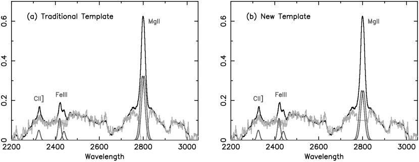
Figure 1: Fits to the composite spectrum composed of spectra with signal-to-noise ratio greater than the median. (a.) The fit using the “traditional” Fe II template, in which the Fe II flux under Mg II is assumed to be zero. (b.) The fit using the “new” template, in which the Fe II flux under Mg II is assumed to be comparable to that adjacent to the line. Note the difference in Mg II flux between the two fits.

A potential problem with this template analysis is that we do not know the flux of the Fe II pseudo-continuum lying directly under Mg II. Traditionally, the template has been set equal to zero in that wavelength range (e.g., Vestergaard & Wilkes, 2001; Dietrich et al., 2003). The possible problem with that procedure is that the gap in the template is fit as part of the Mg II line, and this can affect its width and flux. Therefore, we develop two templates, one in which the Fe II flux is assumed to drop to zero under Mg II (referred to as the “traditional” template), and another in which the Fe II flux is assumed to be approximately the same under Mg II as it is adjacent to the line (referred to as the “new” template). Fig. 1 shows fits to the composite spectrum with both of these templates; the lower flux in the Mg II line for the new template fit can clearly be seen. Thus, we perform much of the analysis in parallel using both templates. Results that are the same for both templates should be robust to the systematic uncertainty of our lack of knowledge of the Fe II flux under Mg II, at least to first order.

We then used the IRAF spectral fitting program Specfit to model the spectra (Kriss, 1994) between 2200 and 3050Å. The model consisted of a power law, the Fe II pseudocontinuum, the Mg II doublet, C II]$\lambda 2325$, and Fe III$\lambda\lambda 2419.3,2438.9$. The Mg II doublet components were constrained to have equal flux and width, and fixed separation. The C II] and Fe III lines were weak, and not present in all objects; therefore we fixed the wavelengths to their rest wavelengths, and fixed the widths to $2000\,\rm km\,s^{-1}$, with the aim of measuring their fluxes and equivalent widths but no other properties. The Specfit output yields a measurement and statistical uncertainty for each parameter.

For a majority of the spectra, the I Zw 1 template modeled the iron fairly well. Objects in which the pseudocontinuum shape appeared significantly different than that of I Zw 1, and objects with exceptional Fe II/Mg II ratios will be discussed in Leighly et al. in prep.

We measured the luminosity of the continuum at 2500Å ($H_{0}=70\rm\,km\,s^{-1}$, $\Omega_{M}=0.3$, $\Lambda_{0}=0.7$), the Fe II and Mg II fluxes, the Mg II and Fe II equivalent widths, and the Mg II velocity width. We computed the black hole mass using the formula presented by McLure & Jarvis (2002), based on the luminosity at 3000Å and the velocity width of Mg II. We estimate the bolometric luminosity using $\lambda L_{\lambda}$ at 2500Å bolometric correction factor of 5.26 (Elvis et al., 1994, their median value). We then compute $L/L_{Edd}$. This will be proportional to Ṁ$/M_{BH}$, assuming that the efficiency of conversion of gravitational potential energy to radiation is the same in all objects. We then discarded 21 more objects due to low signal-to-noise ratio, leaving a sample of 903 objects.

3 Analysis

3.1 Maximum Likelihood Analysis Part 1

We first determine whether there is significant variance in the parameters that we measure, or whether the data is consistent with a constant. To do this, we use the maximum likelihood method (Maccacaro et al., 1988) to determine the mean and dispersion and uncertainties on the following parameters: Mg II equivalent width (EW), Fe II EW, Fe II/Mg II, Mg II/Fe II, Mg II FWHM, $L_{2500}$, $M_{BH}$, and $L/L_{Edd}$. We also investigate the distributions of the luminosities of Mg II and Fe II, because the equivalent width is a function of two physical parameters: the line flux in comparison with the continuum flux, and the covering fraction. The maximum likelihood method computes the best estimate of the mean and dispersion of the data, accounting explicitly for the errors in the data. Thus, a non-zero dispersion implies real variance in the data, not just statistical fluctuations.

The luminosities have somewhat of a large and asymmetric spread, and therefore we discuss the log of these values. Taking the log of a value makes the uncertainties nominally non-symmetric; however, we need a symmetric error for further analysis. We estimate the errors in the logarithm of the value using propagation of errors, taking the first term in the Taylor expansion. To determine the validity of the estimation, we compute the ratio of the second term with the first term. In all cases, that ratio is less than 4%, indicating that the errors are symmetric to within 4%. We deem this acceptably small uncertainty, and henceforth use the first term in the expansion as a symmetric error.

Table 1 lists the results of the maximum likelihood analysis. All of the parameters that we are interested in have dispersions significantly different from zero. This means that there is a real range of values of these parameters.

It is particularly interesting that Fe II/Mg II is not consistent with a constant. Fig. 2 shows the histogram of the Fe II/Mg II values, and Fig. 3 shows the maximum likelihood contours. It is interesting to note that the mean value for the traditional template of 3.93 is quite similar to that found for high redshift quasars (Dietrich et al., 2003). All of these objects have redshifts between 1.2 and 1.8, and at this point, evolution of the iron and magnesium ratios should have ceased (Hamann & Ferland, 1993). Assuming uniform evolution of elements in the host galaxies, and uniform excitation of Fe II and Mg II in all objects, the ratio should be consistent with a constant, in contrast with what we find. We therefore next performed several analyses to determine the origin of the range of values of Fe II/Mg II.

The histogram and contour for the new template are shifted toward higher Fe II/Mg II compared with the results for the traditional template. Comparing maximum-likelihood means for the Mg II and Fe II equivalent widths, we find that the difference lies in the Mg II equivalent widths; they are systematically smaller for the new template, while the means of the Fe II equivalent widths are consistent between the two templates. This is expected, because we expect Mg II equivalent width to grow in step with Fe II equivalent width for the traditional template. This systematic propagates to a larger dispersion in Fe II/Mg II ratio for the new template; the dispersion to mean ratio is 33% for the new template, and 24% for the traditional template.

3.2 Correlations

Table 2 presents the Spearman rank correlation coefficient $r$ for all of the parameters discussed above. We note several apparently strong correlations with $|r|>0.5$: between the Fe II and Mg II equivalent widths, between the line luminosities, between the Fe II line equivalent widths and their luminosities, between the Fe II/Mg II ratio and the Fe II equivalent width and luminosity, between the continuum luminosity and line luminosity, and between the Eddington ratio, black hole mass, the luminosity, and Mg II FWHM.

Do these correlations give us any physical insight, especially for the question of the origin of the range of Fe II/Mg II ratios observed? Specifically, we expect the line and continuum luminosities to be correlated in a flux-limited sample. The fluxes are correlated, and the narrow redshift range does not decorrelate the luminosities. The line equivalent widths are correlated. Since the Fe II and Mg II emission should occur in the same gas, this correlation is expected and may indicate a range of covering fractions; it is also a function of the correlations in fluxes. In addition, the Eddington ratio parameter and black hole mass should be correlated with the continuum luminosity and the Mg II FWHM because they are functions of these two parameters.

There are two potentially physically interesting correlations. The first is an anticorrelation between the Mg II equivalent width and the Eddington ratio. The Eddington ratio parameter is a function of the continuum luminosity and the Mg II FWHM, so one may think that this correlation is a consequence of an anticorrelation between the continuum luminosity and the line equivalent width (the Baldwin effect; Baldwin, 1977) and the correlation between the equivalent width and the velocity width that has been seen previously (e.g., Gaskell, 1985). However, neither of these latter two correlations are particularly strong in this sample, nor are they as strong as the equivalent width and Eddington ratio correlation.

Also interesting is the correlation between the Fe II/Mg II ratio and the Fe II equivalent width ($r=0.62$ for both the traditional and new templates). At first glance, this may appear to be a trivial correlation, because both parameters are positively correlated with the Fe II flux. However, there is no corresponding correlation ($r=0.13$ and 0.33 for the traditional and new templates, respectively) between Mg II EW and Mg II/Fe II.

It is still possible that this correlation is spurious. It is expected that the equivalent width of Mg II should be relatively reliably measured, statistically speaking, because it is a sharp feature. The uncertainty in the equivalent width of Fe II may be larger because it is a broad feature and competes with the continuum. Indeed, the mean relative error of the Fe II equivalent widths is larger than that of the Mg II equivalent widths (6.4% vs 4.0% for the traditional template; 6.4% vs 4.4% for the new template). So, if the Fe II/Mg II ratio were intrinsically constant, a positive fluctuation in Fe II for a particular object would give a positive fluctuation both the ratio and the Fe II equivalent width, with a similar result for a negative fluctuation. The result would be a positive correlation between these parameters, as is seen. An accompanying fluctuation in Mg II would not give rise to as strong of a correlation because it is more securely measured.

On the other hand, a positive correlation might be observed if its origin is physical. Specifically, if the Fe II equivalent width varies more in the sample than the Mg II equivalent width, as a result of a differences in Fe II excitation or iron abundance, a positive correlation between Fe II/Mg II ratio and Fe II equivalent width would also be seen. Indeed, from the maximum likelihood analysis, we find that the dispersion relative to the mean is larger for the Fe II equivalent width compared with the Mg II equivalent width (35% vs 26% for the traditional template; 35% vs 27% for the new template). Since the maximum likelihood analysis accounts for the measurement error, these numbers should reflect real differences in the dispersions of these parameters.

In the next two sections we use simulations and additional maximum likelihood analysis to try to determine whether or not the range of Fe II/Mg II originates in statistical error, or arises in a larger range in values of Fe II EW relative to Mg II EW that may reflect differences in abundance or excitation.

3.3 Simulations

The maximum likelihood analysis indicates that the Fe II/Mg II ratio varies significantly in the sample, and the larger dispersion of Fe II equivalent width relative to Mg II equivalent width suggests that this is the cause of the dispersion in the ratio. However, the uncertainties in the measurements of Fe II EW are about 1.6 times larger than those in Mg II EW, a fact that can also cause a correlation. In this section we present simulations that are designed to test the influence of each factor in turn. We only describe simulations on the traditional template data; the results for the new template are essentially the same.

First we construct samples of simulated Fe II and Mg II equivalent widths and corresponding Fe II/Mg II ratios that have essentially the same distributions as the observed data. The simulated data are constructed in three steps. First, we construct Gaussian distributions for the Fe II and Mg II equivalent widths that have means equal to the observed means, and variances equal to the observed variances times scale factors that are determined as described below.

The next step is construction of the errors. The errors are not simply related to the data because we are using the derived quantity equivalent width; furthermore, the uncertainties in the flux are also not simply related to the flux, because observations are of different length and are made under differing conditions. To zeroth order, the errors are correlated with the data. We assume a linear relationship between the log of each parameter and the log of its error, fit for the slope of the distribution, $\beta$, and use the result to construct the initial errors on the simulated data. Then, because the errors themselves have a large spread for a given value of the data, we randomize them further by adding a Gaussian random variable that has magnitude equal to a constant factor, determined empirically, times the data. The result is that the constructed errors have a variance in $\log_{10}(error)-\beta\log_{10}(data)$ that is only slightly lower than observed.

We next add noise to the data. The noise amplitude is set equal to the square root of the mean square uncertainties.

At this point in the simulation, we have a large number of pairs of Fe II and Mg II equivalent widths or luminosities. However, not all pairs are valid, because the ratio of Fe II to Mg II is not arbitrary in the observed data. We assume a Gaussian distribution of Fe II/Mg II ratio that has the mean and standard deviation of the real data. We partition this distribution into bins of width 0.1 and discretize it. We then pack the distribution with pairs of Fe II and Mg II equivalent width or luminosity, rejecting pairs that are outside the distribution or that fall in a particular bin that is already filled.

Forcing the simulated Fe II/Mg II distribution to match the observed Fe II/Mg II distribution narrows the distributions of the simulated Fe II and Mg II equivalent widths. To account for this, we broaden the initial distribution by the scale factor mentioned above. To determine the value of the scale factors, which are different for Mg II EW and Fe II EW, we require that the variance in the simulated data match that of the original data. These scale factors are determined by running the distribution simulation program 100 times each for a range of initial scale factors, and then determining which scale factor produces the observed variance on average.

Various statistics for the real and these simulated (Simulation 1) data are given in Table 3. We see that, as intended, the distributions, specifically the mean error/data and the maximum likelihood dispersion/mean, are essentially identical.

We list in Table 3 the Spearman rank correlation coefficients between the Fe II EW and the Fe II/Mg II ratio, and between the Mg II EW and the Mg II/Fe II ratio. For both the real data and this first set of simulated data, the correlation coefficient between the Fe II EW and the Fe II/Mg II ratio is much larger than the correlation coefficient between the Mg II EW and the Mg II/Fe II ratio, as expected, because both the dispersion in Fe II equivalent widths and the mean relative error in Fe II EW are larger than those from Mg II.

The second set of simulations (Simulation 2) adjusts the dispersion of the Fe II and Mg II equivalent widths so that ratio of the maximum likelihood values of the dispersion and the mean are approximately equal. This is done by increasing the width of the Mg II EW dispersion, and decreasing the width of the Fe II EW dispersion. The relative errors are kept the same as the original data; now this is the only difference between the Mg II and Fe II simulated equivalent widths. We see that the correlation coefficient between Fe II EW and Fe II/Mg II ratio drops, and the correlation coefficient between Mg II EW and the Mg II/Fe II ratio increases compared with those from Simulation 1 by a large amount, and now they are relatively close together. This suggests that the distribution of the equivalent widths influences the correlations strongly.

In the third set of simulations (Simulation 3), we increase the Mg II equivalent width uncertainty by a factor of 1.6, so that the mean of the relative error is the same for both the Mg II and Fe II equivalent widths. But we leave the maximum likelihood dispersion/mean of the equivalent widths the same as the real data. In this case, we find very little difference in the correlation coefficients compared with Simulation 1, suggesting that the different relative errors in the data influences the correlations very little.

In the final set of simulations (Simulation 4), we make both the dispersions of the Fe II and Mg II equivalent widths, and the relative uncertainty on the Fe II and Mg II equivalent widths equal. In this case we match the straight standard deviation divided by the mean, rather than the maximum likelihood value because although the mean relative uncertainties are set equal, the distribution is somewhat different (see above), and that enters into the maximum likelihood estimation. Regardless, the maximum likelihood estimates of the dispersion/mean are very close (0.29 vs 0.30 for the Mg II EW and Fe II EW, respectively). We find that the correlation coefficient between Fe II EW and Fe II/Mg II is the same as Mg II EW and Mg II/Fe II, as expected, since the factors that influence the correlation coefficient are now equal.

Our conclusions from these simulations is that while both the relative uncertainty and the dispersion of the data can result in positive correlations, the influence of the distribution is much more important in these data; the relative uncertainty has very little influence. So we conclude that the reason that the correlation between Fe II EW and Fe II/Mg II is stronger than that between Mg II EW and Mg II/Fe II is because the dispersion in Fe II EW is larger than that of Mg II EW, and not because the relative uncertainties in the data are larger for Fe II EW compared with Mg II EW.

3.4 Maximum Likelihood Analysis Part 2

The maximum likelihood analysis over the whole sample given in Table 1 shows that the dispersion is significant in Mg II and Fe II equivalent widths, as well as in Fe II/Mg II ratios. In principle, the dispersion in Fe II/Mg II could be produced by a larger spread in Mg II, or a larger spread in Fe II. The fact that the dispersion relative to the mean is larger in Fe II compared with Mg II (35% compared with 26% for the traditional template, 35% compared with 27% for the new template) suggests that Fe II is the culprit. In this section, we investigate this further using a maximum likelihood analysis.

We sort the spectra according to Mg II equivalent width, and divide into nine bins, according to the value of that parameter. We then compute the maximum likelihood estimate of the Fe II/Mg II ratio in each bin. We do the same for Fe II equivalent widths.

The results for the traditional and new templates are shown in Fig. 4. They show that the mean and dispersion of Fe II/Mg II has much different behavior depending on whether they are computed from spectra in bins chosen by their Mg II equivalent width or their Fe II equivalent width. Bins chosen by Fe II equivalent width yield a broad range of maximum-likelihood mean Fe II/Mg II ratios. Bins chosen by Mg II equivalent width yield maximum-likelihood mean Fe II/Mg II ratios almost independent of the Mg II equivalent width. Furthermore, the dispersion of Fe II/Mg II for bins chosen by Mg II equivalent width is similar to the dispersion of Fe II/Mg II in the whole sample. This means that in each Mg II EW bin, a broad range of Fe II/Mg II is present, similar to the whole sample. In contrast, at least for intermediate values of Fe II equivalent width, the dispersion in the Fe II/Mg II ratio drops compared with the whole sample; objects in these bins are more likely to have the same value of Fe II/Mg II ratio. These results imply that Fe II influences the Fe II/Mg II ratio more than Mg II. Recall that the maximum likelihood analysis accounts for the measurement errors in the equivalent widths and ratios, so these results cannot be attributed to the slightly larger relative uncertainties on Fe II parameters.

3.5 Composite Spectra

We next study composite spectra to see if we can obtain some insight on the physical origin of the range of Fe II/Mg II ratios.

First, we sort the observed Fe II/Mg II values, and divide them into nine bins of 100 objects. We then construct composite spectra of the objects in each bin with signal-to-noise ratio greater than the sample median. The resulting composite spectra are composed of between 40 and 65 individual spectra.

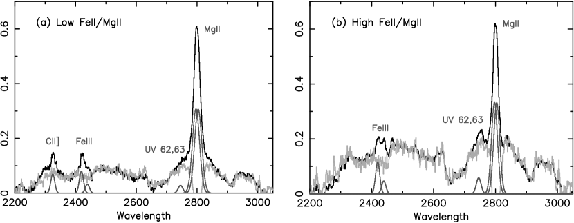
Figure 6: Fits to the two extreme of nine composite spectra accumulated from sorted Fe II/Mg II. Only the results using the traditional template are shown; the results using the new template are essentially identical. (a.) Composite spectrum from the bin containing the lowest values of Fe II/Mg II. (b.) Composite spectrum from the bin containing the highest values of Fe II/Mg II. C II] is much stronger in the low Fe II/Mg II composite.

We then fit each spectrum using the same model as before, except we add an additional line with width fixed at $2000\rm\,km\,s^{-1}$ at 2745.72Å. This component fits the contribution of Fe II UV 62,63 that sometimes appears as a spike in the spectrum. We fit the model twice, using both the traditional and new templates. The fit parameters are plotted as a function of measured Fe II/Mg II ratio in Fig. 5. The fits for the spectra from the lowest and highest Fe II/Mg II ratio bins are shown in Fig. 6.

The results are illuminating. First of all, we confirm our suspicions about the influence of the template on the Mg II properties. While the Mg II equivalent width drops with increasing Fe II/Mg II ratio for both templates, the decrease is less for the traditional template: the standard deviations divided by the means of the composite-spectra Mg II EW are 0.047 and 0.11 for the traditional and new templates, respectively. However, the increase in the Fe II equivalent width as Fe II/Mg II increases is larger than the decrease in Mg II equivalent width: the standard deviations divided by the means are 0.21 and 0.22 for the traditional and new templates respectively. This provides additional evidence that the range of Fe II/Mg II observed is primarily a result of a larger dispersion in Fe II compared with Mg II.

There are several other interesting results. The Mg II FWHM decreases with increasing Fe II/Mg II by $\sim 500\rm\,km\,s^{-1}$ and $\sim 700\rm\,km\,s^{-1}$ for the traditional and new templates, respectively. The difference between the Mg II velocity widths for the two templates is most pronounced for the largest-width Mg II lines, as anticipated, but it was less than $200\rm\,km\,s^{-1}$ in any case, and is zero for the narrowest-width lines. This result appears to imply that, like optical Fe II (e.g., Boroson & Green, 1992), UV Fe II is stronger in objects with narrower lines.

The smaller lines, C II], Fe III, and Fe II UV 62, 63, show interesting trends with Fe II/Mg II ratio. C II] is strongest when the ratio is low, and significantly weaker when the ratio is high, especially for the two spectra with largest Fe II/Mg II. This is interesting, because the properties of this semiforbidden line may give us some clues about the physical (versus phenomenological) origin of the range in Fe II/Mg II ratio (see §4.2). Fe III is weaker when Fe II/Mg II is small, and nearly constant with higher values of this ratio. Finally, Fe II UV 62, 63 is nearly constant with Fe II/Mg II, except it is significantly stronger for the spectrum with the largest Fe II/Mg II ratio.

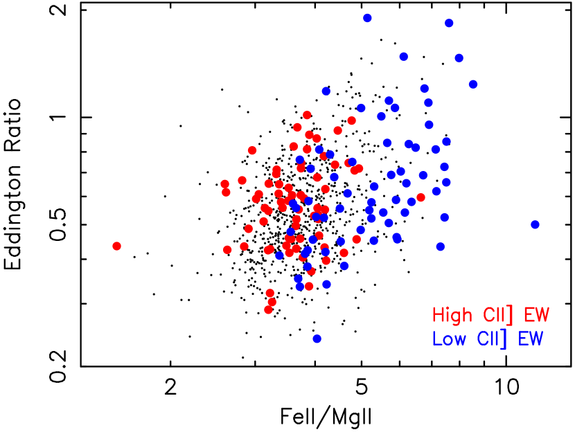
Figure 8: Objects with zero C II] equivalent width (large blue symbols) are more likely to have high Fe II/Mg II ratios, while objects with high C II] equivalent widths (large red symbols) have low or average Fe II/Mg II ratios. Since C II] is sensitive to density, this difference suggests that the range in Fe II/Mg II ratios observed in the sample is a consequence of a range of physical conditions in the emitting gas. Small symbols show the remaining objects in the sample that either have moderate C II] equivalent width lines, or have zero C II] equivalent width lines and low signal-to-noise ratio spectra.

Since C II] is potentially important for understanding the origin of the Fe II/Mg II dispersion, we investigate its properties in another way. We have fitted this line in all of the spectra. It is a weak line, so we can’t simply take the measured equivalent widths at face value; we need to be certain that we are analyzing meaningful detections. To find objects with large C II], we isolate objects in which the C II] flux is not equal to zero and in which the measured flux is more than three times the uncertainty. This leaves 352 objects. From these, we make a composite spectrum from the spectra of the 70 objects with the highest C II] equivalent widths; that composite spectrum is shown in the left panel of Fig. 7. We also need to compile a sample with low values of C II] equivalent width. To do this, we use the 67 objects that have fitted C II] equivalent width equal to zero, and have a signal-to-noise ratio of the spectrum greater than the sample median. That spectrum is shown in the right panel of Fig. 7. We also show the distribution of the high and zero C II] equivalent width objects on the Fe II/Mg II ratio vs Eddington ratio plane, in Fig. 8.

These analyses confirm our finding from the Fe II/Mg II-sliced composite spectra: on average, low (zero) C II] EW objects have high Fe II/Mg II ratios, and high C II] EW objects have low (actually average) Fe II/Mg II ratios. The measured Fe II/Mg II ratio (traditional template) for the high and zero C II] EW composites are 3.5 and 5.1 respectively. Furthermore, we find a distinct separation of the locations of these types of objects on the Fe II/Mg II ratio vs. Eddington ratio parameter plane. Objects with high C II] equivalent widths have average Fe II/Mg II ratios, and objects with high Fe II/Mg II ratios are very likely to have C II] equivalent widths equal to zero. We tentatively interpret this as evidence that the C II] equivalent width and the Fe II/Mg II ratio are coupled such that physical conditions that cause C II] equivalent width to be zero also cause the Fe II/Mg II ratio to be high. Plausible candidates for such physical conditions are discussed below.

4 Discussion

We report the results of analysis of the rest frame 2200–3050Å region in a sample of 903 objects with relatively narrow Mg II lines drawn from the Sloan Digital Sky Survey. We fit the spectra with a model consisting of seven components: a powerlaw continuum, the iron template, and six Gaussians fit to Mg II $\lambda\lambda 2796.4,2803.5$, C II] $\lambda 2325.0$, and Fe II $\lambda\lambda 2419.3,2438.9$. We used two Fe II templates that treat the region under Mg II differently in order to test the effect of our lack of knowledge of the Fe II flux in that region on the results. We discovered that there is a significant range of Fe II/Mg II ratios in the sample: the maximum likelihood means and 1-sigma dispersions are $3.93\pm 0.95$ (traditional Fe II template) and $5.28\pm 1.72$ (new Fe II template). Through simulations, we show that this range, and corresponding correlation between Fe II equivalent width and Fe II/Mg II ratio, are primarily a consequence of a larger dispersion of Fe II EW relative to Mg II EW. This larger dispersion in Fe II EW could be a consequence of a difference in iron abundance, or it could be a consequence of a difference in iron excitation. The latter possibility is supported by our discovery of a coupling between the C II] equivalent width and the Fe II/Mg II ratio. Below, we discuss these two possibilities in turn.

4.1 Iron Abundance

Could the larger range in Fe II equivalent widths originate in real variation in the relative iron and magnesium abundances? At the intermediate redshift range that we investigate, the Universe is already 3.5–5 Gyr old. The models calculated by Hamann & Ferland (1993) show that the abundances of Fe and Mg have almost stopped evolving at this point.

Hamann & Ferland (1992, 1993, 1999) make the case for normal evolution of stellar populations in galactic nuclei for the element enrichment in QSOs. If that is true, we can estimate the spread in [$\alpha$/Fe] expected in the sample, because the black hole mass is related to the stellar velocity dispersion, which is related in turn to [$\alpha$/Fe]; this is related to the mass-metallicity relationship for elliptical galaxies.

We first note that the black holes in our sample of relatively luminous objects are sufficiently large to have elliptical hosts. The mean and dispersion of the black hole masses are $7.3\pm 2.7\times 10^{7}\,M_{\odot}$ and $7.1\pm 3.2\times 10^{7}\,M_{\odot}$ for the traditional and new templates respectively. The spheroid mass is related to the black hole mass by $M_{BH}=0.0012M_{sph}$ (Dunlop, 2004). Thus, the spheroid masses are expected to be around $6\times 10^{10}\,M_{\odot}$, the size of a typical elliptical galaxy.

We have estimated the black hole masses for the sample, using the McLure & Jarvis (2002) formalism. From these, we estimate the stellar velocity dispersion for each object using the formula from Tremaine et al. (2002): $\log(M_{BH}/M_{\odot})=\alpha+\beta\log(\sigma/\sigma_{0})$, where $\sigma_{0}=200\rm\,km\,s^{-1}$, $\alpha=8.13\pm 0.06$, and $\beta=4.02\pm 0.32$. At this point, uncertainties are simply the statistical uncertainties propagated through the equations. We then find the maximum likelihood mean and dispersion of $\sigma$ to be $169\pm 13$ and $166\pm 17\rm\,km\,s^{-1}$ for the traditional and new templates respectively. The small dispersion in these values is a consequence of the relatively narrow range in black hole masses inferred in the sample. We see from Fig. 1 in Thomas, Maraston & Bender (2002) that this velocity dispersion corresponds to [$\alpha$/Fe] of approximately $0.18\pm 0.05$, where the values given are inferred by eye from the figure. This implies that the estimated disperson/mean in the Mg/Fe ratio is reasonably expected to be about 17%. This is somewhat smaller than the 1-sigma dispersion/mean estimate for the sample Fe II/Mg II (24% and 33% for the traditional and new templates, respectively).

Our estimate of the range in $\sigma$ expected in the sample accounted for only statistical uncertainties. McLure & Jarvis (2002) estimate that their black hole masses derived from Mg II FWHM and $L_{3000}$ is good to a factor of 2.5. Our sample may be more uniform than theirs, in which case this systematic error may be an overestimate. Regardless, for the average value of black hole mass of $7.2\times 10^{7}\,\rm M_{\odot}$, a factor of 2.5 higher and lower black hole mass would lead to a $\sigma$ range of 140–210$\,\rm km\,s^{-1}$, corresponding to only a slightly larger disperson in [$\alpha$/Fe] of approximately $0.20\pm 0.1$. This corresponds to an estimated expected mean/dispersion in the Mg/Fe ratio of 23%, comparable to the observed 1-sigma dispersion/mean estimate for the sample Fe II/Mg II.

It is important to realize, however, that a high iron abundance may not be directly observable in the Fe II/Mg II ratio. In other words, a factor of three higher iron/magnesium abundance ratio may not be manifested in a factor of three larger Fe II/Mg II. This is because in classical photoionization models, Fe II has a thermostatic effect (e.g., Collin & Joly, 2000). This means that UV Fe II should not be very sensitive to abundance differences (Verner, 2000; Verner et al., 2003). On the other hand, Verner (2000) shows that not all Fe II lines are affected the same way by changes in abundance because of the accompanying change in optical depth which affects more strongly nearly-saturated emission lines. This implies that we might expect the iron pseudocontinuum to look different in objects with different [Fe/Mg].

In addition, it has also been suggested that objects with high Eddington ratio may have high abundances because rapid star formation may accompany fast growth of the black hole (Mathur, 2000). This has been primarily discussed in the context of nitrogen abundances, which, depending on the star formation model, increase strongly much before or concurrent with iron (Hamann & Ferland, 1993). Assuming that the iron originates in primarily in Type 1a supernovae, it should depend on how long the high accretion rate period has been in progress because of the $\sim 1\,\rm Gyr$ delay. In our sample, $L/L_{Edd}$ parameter is correlated with Fe II/Mg II but not strongly (Fig. 8).

In summary, we find that the expected range in [$\alpha$/Fe] in the elliptical hosts may be sufficient to explain the 1-$\sigma$ dispersion in the observed Fe II/Mg II ratios. This assumes that the abundance ratio is linearly manifested in the line ratio; it may not be, due to the thermostatic effect of Fe II. Regardless, the expected range in abundances is not sufficient to explain the long tail of objects with very high Fe II/Mg II ratios that can be seen in Fig. 2 or Fig. 8.

4.2 Fe II Excitation

Analysis of composite spectra compiled from spectra selected by their Fe II/Mg II ratios (§3.5) shows that high Fe II/Mg II ratios are associated with weak C II] and strong Fe II UV 62,63. Furthermore, we find that objects with measured C II] equivalent widths equal to zero are likely to have enhanced Fe II/Mg II ratios. These results suggest that the range in Fe II/Mg II is a consequence of different excitation of Fe II rather than abundances.

What processes might be responsible for the different excitation? Verner & Peterson (2004) recently show that a high Fe II/Mg II ratio is predicted by their model when the photoionizing flux and density are high. They also find that there is a tendency for higher-luminosity objects to have higher Fe II/Mg II ratios. The nature of the link they infer between the luminosity of an object and the photoionizing flux at the BLR and its density is unclear, however. For constant Eddington ratio, the luminosity, black hole mass, and size of the emission region should all scale together. For variable Eddington ratio, these scalings could change, because the accretion geometry plausibly changes; however, for our sample, we find that the Fe II/Mg II ratio is not strongly correlated with the Eddington ratio. In either case, the spectral energy distribution should change. Also, Verner & Peterson (2004) confine their discussion to the Fe II/Mg II ratio; it is not clear whether their model could naturally explain the correlation of that parameter with Fe II equivalent width that we see.

Alternatively, the difference in the C II] equivalent widths in the high and low Fe II/Mg II composite spectra, and the differences in the distributions of objects with high and zero C II] equivalent widths (§3.5) suggests differences in optical depth or density of the emission-line region. Kwan & Krolik (1981), in an early BLR photoionization model, used the C II]$\lambda 2326$ line as a column density diagnostic, because this low-ionization line is emitted deep in the partially-ionized zone, and because, being a semiforbidden line, it should be less affected by radiative transfer. Following this argument, it could be concluded that the low Fe II/Mg II objects have a high column density which both increases the C II] EW, and decreases the UV Fe II EW as part of the UV Fe II is converted into optical Fe II. This view is supported by the anticorrelation of optical and UV Fe II observed in the PG quasars (Shang et al., 2003) and we note that we can see that C II]$\lambda 2326$ is anticorrelated with UV Fe II in their spectral principal component called (SPC)3.

However, this argument may not be complete. Ferland & Persson (1989) show that C II] will be optically thick in gas that produces Fe II. More important is the fact that C II]$\lambda 2326$ has a rather low critical density of $3.16\times 10^{9}\rm\,cm^{-3}$ (Hamann et al., 2002). This suggests density plays a role, with the low and high Fe II/Mg II objects being characterized by low and high densities, respectively. High density increases Fe II emission because Fe⁺ is primarily excited by collisions. Mg II can decrease at high densities as the line becomes thermalized. Individual Fe II transitions can be saturated at high density, but the large number of transitions available prevents UV Fe II emission as a whole from becoming thermalized, so the Fe II pseudocontinuum increases at high densities (Verner, 2000).

The enhancement of Fe II UV 62, 63, which are transitions that have low-lying upper levels, in high Fe II/Mg II objects may imply that differences in excitation may contribute to the range of Fe II equivalent widths. These Fe⁺ lines have upper levels near 5.5 eV that could be excited by additional heating, perhaps by a mechanical source (e.g., Collin & Joly, 2000). The photoionizing flux can influence the emission from the lowest levels, because if the flux is low, the partially ionized zone is thin, and the lines from the low-lying levels are not saturated and appear stronger (Verner, 2000). Microturbulence could also enhance the emission from the low-lying levels, because it reduces the effective optical depth (Sigut & Pradhan, 2003). Evidence for microturbulence in NLS1s has already been seen; the enhancement of Fe III$\lambda 1914$ in several NLS1s quite likely arises from pumping by Ly$\alpha$ (Leighly & Moore, 2004; Johansson et al., 2000). The upper level energy for Fe III$\lambda 1914$ corresponds to 1214.6Å, which is 1.1Å from Ly$\alpha$, implying a velocity difference of $274\,\rm km\,s^{-1}$.

It is also possible that the spectral energy distribution (SED) can affect the Fe II emission. A SED with strong hard X-ray emission can increase the depth of the partially-ionized zone, and increase the Fe II emission (e.g., Collin & Joly, 2000). A very soft SED may also be able to influence the production of Fe II emission as well. A soft SED may increase the depth of the partially ionized zone by free-free absorption if it is strong in the IR (Ferland & Persson, 1989). In a gas photoionized by a very soft SED, there will be few highly-ionized ions, because the SED lacks the photons required by their high ionization potential. The gas will be dominated by low-ionization ions, such as H⁺ and Fe⁺, and Ly$\alpha$ emission will be strong. If microturbulence is present, Ly$\alpha$ pumping of Fe II may be very strong. Mg II would not be similarly enhanced. In this case, the Fe II pseudocontinuum may be dominated by high-excitation transitions. This may be responsible for the ultra-strong Fe II emission observed in the narrow-line quasar PHL 1811 (Leighly, Halpern & Jenkins, 2004, Leighly et al., in prep.) and in some of the SDSS objects (Leighly et al., in prep.).

Figure 2: Histograms of the measured Fe II/Mg II ratios. Solid: traditional Fe II template; Dashed: new Fe II template. Note that an exceptional object with a measure Fe II/Mg II ratio of 33.5 for the new template is not shown.

Figure 3: Maximum likelihood-analysis contours for Fe II/Mg II. Solid: traditional Fe II template; Dashed: new Fe II template. Contours are 68%, 90%, and 99% for two parameters of interest. The fact that the dispersion in this parameter is significantly greater than zero demonstrates that there is a significant range in this ratio in the sample.

Figure 4: Maximum likelihood contours of the mean and dispersion of Fe II/Mg II from nine bins from sorted Mg II equivalent width (top) and sorted Fe II equivalent width (bottom). Only the 99% contour is shown for clarity. Contour shade gradient runs from dark to light for small to large values of the parameter. (a.) Results from fits using the traditional Fe II template; (b.) Results from fits using the new Fe II template.

Figure 5: Spectral fitting results for the nine composite spectra obtained by sorting Fe II/Mg II values, splitting into nine bins, and accumulating spectra that have signal-to-noise ratio greater than the median value. (a.) Results from fits using the traditional Fe II template; (b.) Results from fits using the new Fe II template.

Figure 7: Composite spectra compiled from spectra with high (left) and low (right) equivalent width C II] lines.

Table 1: Maximum Likelihood Analysis

	Traditional Fe II Template		New Fe II Template
Parameter	Mean	1$\sigma$ Dispersion	Mean	1$\sigma$ Dispersion
Mg II EW (Å)	$22.42^{+0.59}_{-0.61}$	$5.85^{+0.47}_{-0.41}$	$18.00\pm 0.50$	$4.88^{+0.39}_{-0.35}$
$\log\rm L_{MgII}$	$42.80\pm 0.02$	$0.22\pm 0.02$	$42.70\pm 0.02$	$0.22\pm 0.02$
Fe II EW (Å)	$87.7\pm{3.1}$	$30.4^{+2.5}_{-2.2}$	$92.8\pm 3.3$	$32.1^{+2.6}_{-2.3}$
$\log\rm L_{FeII}$	$43.39\pm 0.03$	$0.25\pm 0.02$	$43.41\pm 0.03$	$0.25\pm 0.02$
Fe II/Mg II	$3.93\pm 0.10$	$0.95^{+0.08}_{-0.07}$	$5.28\pm 0.18$	$1.72^{+0.14}_{-0.13}$
Mg II/Fe II	$0.263\pm 0.006$	$0.053^{+0.005}_{-0.004}$	$0.202^{+0.006}_{-0.005}$	$0.051\pm 0.004$
Mg II FWHM ($\rm\,km\,s^{-1}$)	$2635\pm 35$	$340^{+30}_{-20}$	$2576\pm 48$	$460^{+40}_{-30}$
$\log\rm L_{2500}$	$41.53\pm+0.02$	$0.21^{+0.02}_{-0.01}$	$41.53^{+0.022}$	$0.21^{+0.02}_{-0.01}$
$M_{BH}$	$7.31\pm 0.28\times 10^{7}$	$2.73^{+0.21}_{-0.19}\times 10^{7}$	$7.08^{+0.33}_{-0.32}\times 10^{7}$	$3.17^{+0.25}_{-0.23}\times 10^{7}$
Eddington Ratio	$0.58\pm 0.02$	$0.21\pm 0.02$	$0.62\pm 0.03$	$0.28\pm 0.02$

Note. — Quoted uncertainties are 99% confidence for two parameters of interest ($\Delta\chi^{2}=9.21$).

Table 2: Correlation Matrix

	Mg II EW	Fe II EW	$\log(L_{MgII})$	$\log(L_{FeII})$	Fe II/Mg II	Mg II/Fe II	Mg II FWHM	$\rm L_{2500}$	$M_{BH}$	$L/L_{Edd}$
Mg II EW	1.00	0.69	0.28	0.20	$-$0.13	0.13	0.29	$-$0.23	0.05	$-$0.41
	1.00	0.51	0.30	0.09	$-$0.33	0.33	0.36	$-$0.24	0.16	$-$0.48
Fe II EW	0.69	1.00	0.28	0.48	0.56	$-$0.56	0.02	$-$0.08	$-$0.04	$-$0.09
	0.51	1.00	0.21	0.49	0.56	$-$0.56	$-$0.01	$-$0.08	$-$0.06	$-$0.05
$\log(L_{MgII})$	0.28	0.28	1.00	0.90	0.06	$-$0.06	0.32	0.84	0.73	0.37
	0.30	0.21	1.00	0.83	$-$0.07	0.07	0.37	0.82	0.70	0.17
$\log(L_{FeII})$	0.20	0.48	0.90	1.00	0.43	$-$0.43	0.16	0.79	0.58	0.47
	0.09	0.49	0.83	1.00	0.43	$-$0.43	0.14	0.79	0.49	0.37
Fe II/Mg II	$-$0.13	0.56	0.06	0.43	1.00	$-$1.00	$-$0.32	0.12	$-$0.14	0.34
	$-$0.33	0.56	$-$0.07	0.43	1.00	$-$1.00	$-$0.37	0.12	$-$0.23	0.40
Mg II/Fe II	0.13	$-$0.56	$-$0.06	$-$0.43	$-$1.00	1.00	0.32	$-$0.12	0.14	$-$0.34
	0.33	$-$0.56	0.07	$-$0.43	$-$1.00	1.00	0.37	$-$0.12	0.23	$-$0.40
Mg II FWHM	0.29	0.02	0.32	0.16	$-$0.32	0.32	1.00	0.18	0.78	$-$0.64
	0.36	$-$0.01	0.37	0.14	$-$0.37	0.37	1.00	0.17	0.86	$-$0.77
$\rm L_{2500}$	$-$0.23	$-$0.08	0.84	0.79	0.12	$-$0.12	0.18	1.00	0.71	0.59
	$-$0.24	$-$0.08	0.82	0.79	0.12	$-$0.12	0.17	1.00	0.62	0.44
$M_{BH}$	0.05	$-$0.04	0.73	0.58	$-$0.14	0.14	0.78	0.71	1.00	$-$0.07
	0.16	$-$0.06	0.70	0.49	$-$0.23	0.23	0.86	0.62	1.00	$-$0.36
$\rm L/L_{Edd}$	$-$0.41	$-$0.09	0.37	0.47	0.34	$-$0.34	$-$0.64	0.59	$-$0.07	1.00
	$-$0.48	$-$0.05	0.17	0.37	0.40	$-$0.40	$-$0.77	0.44	$-$0.36	1.00

Note. — Correlation coefficient is Spearman Rank. For each entry, the upper and lower numbers are from analyses using the traditional and new iron templates, respectively.

Table 3: Simulation Results

Parameter	Real	Simulation 1	Simulation 2	Simulation 3	Simulation 4
Distribution of Data
Mg II EW Mean$\pm$ Standard Dev.	$22.5\pm 6.1$	$22.6\pm 6.4$	$22.7\pm 7.0$	$22.4\pm 5.5$	$22.7\pm 7.0$
ML Mg II EW Mean$\pm$ Standard Dev.	$22.4\pm 5.9$	$22.5\pm 6.3$	$22.6\pm 6.8$	$22.2\pm 5.2$	$22.5\pm 6.5$
Fe II EW Mean$\pm$ Standard Dev.	$88\pm 32$	$88\pm 30$	$87\pm 28$	$87\pm 27$	$87\pm 27$
ML Fe II EW Mean$\pm$ Standard Dev.	$88\pm 30$	$87\pm 29$	$87\pm 27$	$87\pm 27$	$86\pm 26$
Fe II/Mg II Mean$\pm$ Standard Dev.	$3.9\pm 1.0$	$3.9\pm 1.0$	$3.95\pm 0.96$	$3.95\pm 0.95$	$3.95\pm 0.96$
ML Fe II/Mg II Mean$\pm$ Standard Dev.	$3.93\pm 0.95$	$3.92\pm 0.91$	$3.92\pm 0.91$	$3.90\pm 0.89$	$3.90\pm 0.89$
Derived Distribution Properties
Mg II EW Standard Dev./Mean	0.27	0.28	0.31	0.25	0.31
ML Mg II EW Standard Dev./Mean	0.26	0.28	0.30	0.23	0.29
Fe II EW Standard Dev./Mean	0.36	0.34	0.32	0.31	0.31
ML Fe II EW Standard Dev./Mean	0.35	0.33	0.31	0.31	0.30
Fe II/Mg II Standard Dev./Mean	0.26	0.26	0.24	0.24	0.24
ML Fe II/Mg II Standard Dev./Mean	0.24	0.23	0.23	0.23	0.23
Mean Mg II EW Error/EW	0.040	0.037	0.036	0.059	0.059
Mean Fe II EW Error/EW	0.064	0.060	0.059	0.059	0.060
Correlations
Correlation between Fe II EW and Fe II/Mg II	0.56	0.57	0.43	0.61	0.42
Correlation between Mg II EW and Mg II/Fe II	0.13	0.21	0.36	0.24	0.41

References

- Abazajian et al. (2003) Abazajian, K., et al., 2003, AJ, 126, 2081
- Baldwin (1977) Baldwin, J. A., 1977, ApJ, 214, 679
- Boroson & Green (1992) Boroson, T. A., & Green, R. F., 1992, ApJS, 80, 109
- Collin & Joly (2000) Collin, S., & Joly, M. 2000, New A Rev., 44, 531
- Corbin & Boroson (1996) Corbin, M. R., & Boroson, T. A., 1996, ApJS, 107, 69
- Dietrich et al. (2002) Dietrich, M., Hamann, F., Shields, J. C., Constantin, A., Vestergaard, M., Chaffee, F., Foltz, C. B., & Junkkarinen, V. T., 2002, ApJ, 581, 912
- Dietrich et al. (2003) Dietrich, M., Hamann, F., Appenzeller, I., & Vestergaard, M., 2003, ApJ, 596, 817
- Dunlop (2004) Dunlop, J. S. 2004, In Coevolution of Black holes and Galaxies, ed. L. C. Ho (Cambridge: Cambridge Univ. Press)
- Elvis et al. (1994) Elvis, M., Wilkes, B. J., McDowell, J. C., Green, R. F., Bechtold, J., Willner, S. P., Oey, M. S., Polomski, E., & Cutri, R., 1994, ApJS, 95, 1
- Forster et al. (2001) Forster, K., Green, P. J., Aldcroft, T. L., Vestergaard, M., Foltz, C. B., & Hewitt, P. C., 2001, ApJS, 134, 35
- Ferland & Persson (1989) Ferland, G., & Persson, S. E., 1989, ApJ, 347, 656
- Gaskell (1985) Gaskell, C. M., 1985, ApJ, 291, 112
- Goodrich (1989) Goodrich, R. W. 1989, ApJ, 342, 224
- Hamann & Ferland (1992) Hamann, F., & Ferland, G., 1992, ApJ, 391, 53
- Hamann & Ferland (1993) Hamann, F., & Ferland, G., 1993, ApJ, 418, 11
- Hamann & Ferland (1999) Hamann, f., & Ferland, G., 1999, ARA&A, 37, 487
- Hamann et al. (2002) Hamann, F., Korista, K. T., Ferland, G. J., Warner, C., & Baldwin, J., 2002, ApJ, 564, 592
- Johansson et al. (2000) Johansson, S., Zethson, T., Hartman, H., Ekberg, J. O., Ishibashi, K., Davidson, K., & Gull, T., 2000, A&A, 361, 977
- Heger & Woosley (2002) Hegar, A., & Woosley, S. E., 2002, ApJ, 567, 532
- Joly (1993) Joly, M., 1993, Ann. Phys. Fr., 18, 241
- Kriss (1994) Kriss, G. A. 1994, in Astronomical Data Analysis Software & Systems III, A.S.P. Conf. Series, Vol. 61, eds. D. R. Crabtree, R. J. Hanisch, & J. Barnes (Astronomical Society of the Pacific: San Francisco), p. 437
- Kwan & Krolik (1981) Kwan, J., & Krolik, J. H., 1981, ApJ, 250, 478
- Leighly (1999) Leighly, K. M., 1999, ApJS, 125, 297
- Leighly, Halpern & Jenkins (2004) Leighly, K. M., Halpern, J. P., & Jenkins, E. B., 2004, in Proc. “AGN Physics with the Sloan Digital Sky Survey”, eds. G. T. Richards & P. B. Hall, astro-ph/0402535
- Leighly & Moore (2004) Leighly, K. M., & Moore, J. R., 2004, ApJ, 611, 107
- Maccacaro et al. (1988) Maccacaro, T., Gioia, I. M., Wolter, A., Zamorani, G., & Stocke, J. T. 1988, ApJ, 326, 680
- Mathur (2000) Mathur, S., 2000, MNRAS, 314, 17p
- McLure & Jarvis (2002) McLure, R. J., & Jarvis, M. J., 2002, MNRAS, 337, 109
- Nomoto, Nakamura, Kobashi (1992) Nomoto, K., Nakamura, T., & Kobayashi, C., 1999, ApJS, 265, 37
- Osterbrock & Pogge (1985) Osterbrock, D. E., & Pogge, R. W., 1985, ApJ, 297, 166
- Richards et al. (2002) Richards, G. R., et al., 2002, AJ, 123, 2945
- Shang et al. (2003) Shang, Z., Wills, B. J., Robinson, E. L., Wills, D., Laor, A., Xie, B., & Yuan, J., 2003, ApJ, 586, 52
- Sigut & Pradhan (2003) Sigut, T. A. A., & Pradhan, A. K., 2003, ApJS, 145, 15
- Thomas, Maraston & Bender (2002) Thomas, D., Maraston, C., & Bender, R., 2002, ApSS, 281, 371
- Tremaine et al. (2002) Tremaine, S., et al. 2002, ApJ, 574, 740
- Verner (2000) Verner, E., 2000, Ph. D. Thesis, University of Toronto
- Verner et al. (1999) Verner, E. M., Verner, D. A., Korista, K. T., Ferguson, J. W., Hamann, F., & Ferland, G. J., 1999, ApJS, 120, 101
- Verner et al. (2003) Verner, E., Bruhweiler, F., Verner, D., Johansson, S., & Gull, T., 2003, ApJ, 592, 59
- Verner & Peterson (2004) Verner, E., & Peterson, B. A., 2004, ApJL, 608, 85
- Vestergaard & Wilkes (2001) Vestergaard, M., & Wilkes, B. J., 2001, ApJS, 134, 1