Simulation of non-Gaussian CMB maps

Abstract

A simple method is presented for the rapid simulation of statistically-isotropic non-Gaussian maps of CMB temperature fluctuations with a given power spectrum and analytically-calculable bispectrum and higher-order polyspectra. The $n$th-order correlators of the pixel values may also be calculated analytically. The cumulants of the simulated map may be used to obtain an expression for the probability density function of the pixel temperatures. The statistical properties of the simulated map are determined by the univariate non-Gaussian distribution from which pixel values are drawn independently in the first stage of the simulation process. We illustrate the method using a non-Gaussian distribution derived from the wavefunctions of the harmonic oscillator. The basic simulation method is easily extended to produce non-Gaussian maps with a given power spectrum and diagonal bispectrum.

1 Introduction

The study of non-Gaussianity of Cosmic Microwave Background (CMB) fluctuations is of major importance in understanding the processes responsible for generating the fluctuations and in assessing the contribution of foreground astrophysical processes and instrumental effects to observations of the CMB.

Single-field inflationary scenarios predict, in general, that CMB fluctuations are very nearly Gaussian (see e.g. Bartolo et al. 2004 for a recent review), if one assumes that the sub-Hubble-scale quantum fluctuations start off in the ground state (Contaldi, Bean & Magueijo, 1999; Martin, Riazuelo & Sakellarioudou, 2000; Gangui, Martin & Sakellarioudou, 2002). In such models, non-Gaussianity produced during inflation arises predominantly from the non-linear nature of gravitational interactions rather than from self-interaction of the fluctuations of the inflaton field. Typically the level of non-Gaussianity is suppressed by the first-order slow-roll parameters (Acquaviva et al., 2003; Maldacena, 2003). Subsequent non-linear processing of the primordial fluctuations to second-order in perturbation theory has been shown to amplify the tiny primordial non-Gaussianity to a level on the last-scattering surface that may be detectable with future CMB surveys (Bartolo et al., 2004). Furthermore, second-order radiative transfer effects, such as gravitational lensing of the CMB, should produce a detectable level of non-Gaussianity in the CMB (Zaldarriaga, 2000). Larger levels of non-Gaussianity can be produced in inflation models with multiple scalar fields. Examples include the curvaton (e.g. Lyth & Wands 2002) and the inhomogeneous reheating (e.g. Dvali, Gruzinov & Zaldarriaga 2004) scenarios. Finally models which include topological defects also produce significantly non-Gaussian fluctuations (Gangui, Pogosian & Winitzki, 2002). It is also the case that inevitable contaminants, such as discrete radio sources, Galactic emission and systematic instrumental effects leave non-Gaussian signatures on CMB maps. Thus non-Gaussianity tests are of fundamental importance both for probing inflation physics and for isolating systematic effects.

In order to investigate one’s ability to detect and recover non-Gaussian signals, it is useful to generate non-Gaussian maps with known statistical properties, to which putative analysis methods may be applied. In particular, in many applications, it is desirable that the simulated non-Gaussian map is statistically isotropic, with a prescribed power spectrum (or 2-point correlation function). The generation of such non-Gaussian CMB maps is, however, a surprisingly difficult task (see, for example, Vio et al. 2001, 2002). Moreover, it is often useful for the non-Gaussian map also to have a known (or prescribed) bispectrum and one-point marginal probability density function. Several different techniques have been proposed to address various subsets of these requirements (Contaldi & Magueijo, 2001; Martínez-González et al., 2002; Komatsu et al., 2003; Liguori et al., 2003), but each carries a considerable computational cost. The aim of this paper is to present a simple, fast technique for simulating statistically-isotropic non-Gaussian CMB maps with a prescribed power spectrum, for which one can calculate analytically the bispectrum, higher-order polyspectra, $n$th order pixel correlators and the one-dimensional marginalised distribution (in terms of its cumulants). Moreover, our basic simulation method is easily extended to produce non-Gaussian maps with a given power spectrum and diagonal bispectrum.

The problem of simulating non-Gaussian CMB maps can be formalised as follows. A real, random scalar field $T(\textbf{{x}})$ can be defined as a collection of random variables, one at each point $\textbf{{x}}=(x_{1},x_{2},\ldots,x_{n})$ in the $n$-dimensional space (clearly $n=2$ for CMB maps on the sphere or flat-patches of sky). Thus, for each position x, $T(\textbf{{x}})\equiv t$, where $t$ is a scalar random variable with a one-dimensional (marginal) probability density function (PDF) $f_{T}(t)$. For a random field that is statistically homogeneous, $f_{T}(t)$ is the same at all points in the space. The main difficulty in the numerical simulation of a generic random field is that, in general, given two arbitrary positions $\textbf{{x}}_{1}$ and $\textbf{{x}}_{2}$, the quantities $T(\textbf{{x}}_{1})$ and $T(\textbf{{x}}_{2})$ are not independent. In particular, it is often desirable for $T(\textbf{{x}})$ to have a prescribed 2-point covariance function

$$\xi_{T}(\textbf{{x}}_{1},\textbf{{x}}_{2})=\langle T(\textbf{{x}}_{1})T(\textbf{{x}}_{2})\rangle.$$

In the case of a statistically homogeneous random field in Euclidean space, the covariance function depends only on $\mn@boldsymbol{\tau}\equiv\textbf{{x}}_{1}-\textbf{{x}}_{2}$. If the field is also isotropic then the dependence is only on $\tau=|\mn@boldsymbol{\tau}|$.

As discussed by Vio et al. 2001, 2002, most methods for simulating non-Gaussian maps with a prescribed 2-point covariance function [and a prescribed marginal PDF $f_{T}(t)$] are based on first generating a zero-mean, unit-variance Gaussian random field $G(\textbf{{x}})$, with an appropriate covariance structure $\xi_{G}(\tau)$. One then performs the mapping transformation $G(\textbf{{x}})\to T(\textbf{{x}})$ according to

$$T(\textbf{{x}})=h[G(\textbf{{x}})],$$

where $h$ represents an appropriate function. The usefulness of this approach derives from the fact that there exist explicit analytical (but complicated) formulae for the marginal PDF, $f_{T}(t)$, and the covariance function, $\xi_{T}(\tau)$, of the transformed field in terms of the covariance function, $\xi_{G}(\tau)$, of the original Gaussian field and the mapping function $h$. In particular, we note that the formula for $\xi_{T}(\tau)$ takes the form of a double integral of a function depending on both $\xi_{G}(\tau)$ and $h$. There exist only a few mapping functions $h$ for which $f_{T}(t)$ and $\xi_{T}(\tau)$ may be calculated analytically. A still smaller subset of these cases allows the resulting expressions to be inverted analytically to obtain the required functions $\xi_{G}(\tau)$ and $h$ to be used in simulating the non-Gaussian map. In general, one has to resort to numerical methods to invert the general formulae for $f_{T}(t)$ and $\xi_{T}(\tau)$ and this can be computationally very costly.

As mentioned above, it is often desirable for the simulated non-Gaussian map also to have a known (or prescribed) bispectrum. The method outlined above has not been extended to this case, and any such generalisation is likely to be extremely computationally demanding. An alternative method for generating non-Gaussian maps with a prescribed power spectrum and bispectrum has been suggested by Contaldi & Magueijo (2001), although, in general, the marginal distribution $f_{T}(t)$ of the resulting map cannot be obtained analytically. The method is based on choosing some one-dimensional non-Gaussian PDF, from which the real and imaginary parts of (some subset of) the spherical harmonic coefficients $a_{\ell m}$ of the map are drawn independently (the remaining coefficients being drawn from a Gaussian PDF). However, statistical isotropy imposes ‘selection rules’ upon correlators of the $a_{\ell m}$ coefficients. For example, the third-order correlators must satisfy

$$\langle a_{\ell_{1}m_{1}}a_{\ell_{2}m_{2}}a_{\ell_{3}m_{3}}\rangle=\left(\begin{array}[]{ccc}\ell_{1}&\ell_{2}&\ell_{3}\\ m_{1}&m_{2}&m_{3}\end{array}\right)B_{\ell_{1}\ell_{2}\ell_{3}},$$

where $(\cdots)$ denotes the Wigner $3j$ symbol and $B_{\ell_{1}\ell_{2}\ell_{3}}$ are the bispectrum coefficients. Hence the map corresponding to the drawn $a_{\ell m}$ values is not only non-Gaussian but also anisotropic since all its third-order correlators are zero, except for a subset of the form $\langle a_{\ell m}^{3}\rangle$ for those $a_{\ell m}$ drawn from the non-Gaussian PDF. It is therefore necessary first to produce an ensemble of non-Gaussian, anisotropic maps and then create an isotropic ensemble by applying a random rotation to each realisation. Contaldi & Magueijo (2001) show that these random rotations produce the necessary correlations between the $a_{\ell m}$ coefficients to ensure isotropy of the ensemble, but the method clearly requires significant computation.

In this paper, we discuss a very simple and computationally fast method for simulating non-Gaussian maps that are, by construction, statistically isotropic, and for which numerous statistical properties may be calculated analytically. In particular, it is possible to produce a map with a prescribed power spectrum for which one can obtain simple analytical expressions for the bispectrum and higher-order polyspectra, and $n$th-order correlators of the pixel values. One may also calculate the cumulants of the map, which may be used to obtain the one-dimensional marginalised distribution. A simple extension of the method allows for the simulation of maps with a prescribed power spectrum and diagonal bispectrum. In Section 2, we discuss our method for simulating non-Gaussian maps, the statistical properties of which are presented in Section 3. In Section 4 we extend the method to allow simulation of maps with prescribed power spectrum and diagonal bispectrum. Finally, our conclusions are presented in Section 5.

2 Simulation method

Since our goal is the simulation of CMB maps for use in later analysis, it is convenient at the outset to divide the celestial sphere into pixels labelled by $p=1,2,\ldots,N_{\rm pix}$. For simplicity, we also assume an equal-area pixelisation, so that each pixel subtends the same solid angle $\Omega_{\rm pix}=4\pi/N_{\rm pix}$. Examples of such pixelisation schemes are Healpix (Górski et al. 1999) and Igloo (Crittenden 2000). The distribution of pixel centres across the sphere is unimportant.

Our simulation method begins by drawing each pixel value $s_{p}\equiv S(\textbf{{x}}_{p})=S(\theta_{p},\phi_{p})$ independently from the same one-dimensional non-Gaussian PDF $f_{S}(s)$. The precise PDF used is unimportant, but for the purposes of illustration, we adopt here a PDF derived from the Hilbert space of a linear harmonic oscillator, as developed by Rocha et al. (2001). This class of PDF is summarised in Appendix A. In particular, we assume the PDF illustrated in Fig. 1, which is chosen for convenience to have a mean of zero.

Figure 1: The non-Gaussian PDF used in the simulations (solid line), which has the form given in equation (51) with $\alpha_{3}=0.2$ and $\sigma_{0}=1$, and a set of samples drawn from the PDF (histogram).

The resulting map $S(\textbf{{x}})$ will, by construction, be statistically isotropic to within the errors introduced by the pixelisation scheme. In fact, it is a realisation of isotropic non-Gaussian white noise, with a variance given by the second (central) moment $\mu_{2}$ of the PDF $f_{S}(s)$. We will assume throughout that the mean $\mu_{1}$ of the generating non-Gaussian PDF is zero, so that moments and central moments coincide. According to the ‘cumulant expansion theorem’ (Ma, 1985) the cumulants, or connected moments, of the multivariate distribution of pixel values are related to the logarithm of the moment-generating function,

$$M(\textbf{{k}})\equiv\langle\mathrm{e}^{\mathrm{i}\textbf{{s}}\cdot\textbf{{k}}}\rangle,$$ (1)

where $\textbf{{s}}\equiv(s_{1},\dots,s_{N_{\mathrm{pix}}})$ is the vector of pixel values and $\textbf{{k}}\equiv(k_{1},\dots,k_{N_{\mathrm{pix}}})$. The connected moments are given in terms of the derivatives of $\ln M(\textbf{{k}})$ by

$$\left<s_{p_{1}}\cdots s_{p_{n}}\right>_{c}=(-\mathrm{i})^{n}\frac{\partial^{n}}{\partial k_{p_{1}}\cdots\partial k_{p_{n}}}\ln M(\textbf{{k}})\Big{|}_{\textbf{{k}}=0}.$$ (2)

Given that the pixel values $s_{p}$ are independent random variables we have $\ln M(\textbf{{k}})=\sum_{p}\ln M_{S}(k_{p})$, where

$$\ln M_{S}(k) \equiv \ln\langle\mathrm{e}^{\mathrm{i}sk}\rangle=\ln\int_{-\infty}^{\infty}f_{S}(s)\mathrm{e}^{\mathrm{i}sk}\,\mathrm{d}s$$ (3)

$$= \sum_{n=1}^{\infty}\frac{(\mathrm{i}k)^{n}}{n!}\kappa_{n}$$

is the logarithm of the moment-generating function (the cumulant-generating function) for the non-Gaussian PDF $f_{S}(s)$ whose cumulants are the $\kappa_{n}$. Substituting in equation (2), we find

$$\left<s_{p_{1}}\cdots s_{p_{n}}\right>_{c}=\delta_{{p_{1}}\cdots{p_{n}}}(-\mathrm{i})^{n}\frac{\mathrm{d}^{n}}{\mathrm{d}k^{n}}\ln M_{S}(k)\Big{|}_{k=0}=\delta_{{p_{1}}\cdots{p_{n}}}\kappa_{n}.$$ (4)

The symbol $\delta_{p_{1}\cdots p_{n}}$ equals one if all the $n$ pixels are the same and vanishes otherwise. If required, the pixel correlations can always be expanded in their connected parts (Ma, 1985). In particular, since $\langle s_{p}\rangle=0$ for each pixel, one finds that, for example,

$$\langle s_{p_{1}}s_{p_{2}}\rangle = \langle s_{p_{1}}s_{p_{2}}\rangle_{c}$$

$$\langle s_{p_{1}}s_{p_{2}}s_{p_{3}}\rangle = \langle s_{p_{1}}s_{p_{2}}s_{p_{3}}\rangle_{c}$$

$$\langle s_{p_{1}}s_{p_{2}}s_{p_{3}}s_{p_{4}}\rangle = \langle s_{p_{1}}s_{p_{2}}s_{p_{3}}s_{p_{4}}\rangle_{c}+\langle s_{p_{1}}s_{p_{2}}\rangle_{c}\langle s_{p_{3}}s_{p_{4}}\rangle_{c}$$

$$+\langle s_{p_{1}}s_{p_{3}}\rangle_{c}\langle s_{p_{2}}s_{p_{4}}\rangle_{c}+\langle s_{p_{1}}s_{p_{4}}\rangle_{c}\langle s_{p_{2}}s_{p_{3}}\rangle_{c}.$$

The next step in the simulation procedure is to transform the map $S(\textbf{{x}})$ into spherical-harmonic space (using, for example, the map2alm routine from the Healpix package) to obtain the coefficients

$$a_{\ell m}=\sum_{p=1}^{N_{\rm pix}}Y^{*}_{\ell m}(\textbf{{x}}_{p})s_{p}\Omega_{\rm pix}\approx\int_{4\pi}Y^{*}_{\ell m}(\theta,\phi)S(\theta,\phi)\,\mathrm{d}\Omega.$$ (5)

Using equation (4) and the (approximate) orthogonality of the (pixelised) spherical harmonics, we quickly find that the second-order correlator of the harmonic coefficients is given by

$$\langle a_{\ell m}a^{*}_{\ell^{\prime}m^{\prime}}\rangle=\mu_{2}\Omega_{\rm pix}\delta_{\ell\ell^{\prime}}\delta_{mm^{\prime}},$$ (6)

where $\mu_{2}=\kappa_{2}$ since $f_{S}(s)$ has vanishing mean. In order to obtain a final non-Gaussian map with a particular prescribed ensemble-average power spectrum, $C_{\ell}$, one then rescales the harmonic coefficients to obtain

$$\bar{a}_{\ell m}=a_{\ell m}\sqrt{\frac{C_{\ell}}{\mu_{2}\Omega_{\rm pix}}},$$ (7)

such that $\langle\bar{a}_{\ell m}\bar{a}^{*}_{\ell^{\prime}m^{\prime}}\rangle=C_{\ell}\delta_{\ell\ell^{\prime}}\delta_{mm^{\prime}}$. We note that the effect of a spatially-invariant, circularly-symmetric observing beam on the final map is trivially included by letting $C_{\ell}\to C_{\ell}B_{\ell}^{2}$, where $B_{l}$ are the coefficients of the beam in a Legendre expansion. Finally, the harmonic coefficients $\bar{a}_{\ell m}$ are inverse spherical harmonic transformed (using, for example, the alm2map routine from the Healpix package) to obtain the final map

$$t_{p}\equiv T(\textbf{{x}}_{p})=\sum_{\ell,m}\,\bar{a}_{\ell m}Y_{\ell m}(\textbf{{x}}_{p}),$$ (8)

where the double summation extends from $\ell=0$ to $\ell_{\rm max}$ and $m=-\ell$ to $\ell$. The equivalent flat-sky approximation for small patches is discussed in Appendix C.

In Fig. 2 we plot a realisation of a non-Gaussian all-sky CMB map generated as described above, using the non-Gaussian PDF plotted in Fig. 1 with a prescribed ensemble-average power spectrum, $C_{\ell}$. The map was produced using the Healpix pixelisation scheme with the $N_{\mathrm{side}}$ parameter set to 512, which corresponds to $N_{\mathrm{pix}}=12N_{\mathrm{side}}^{2}\approx 3\times 10^{6}$ equal-area pixels. For comparison, in Fig. 3, we plot a realisation of a Gaussian CMB map with the same power spectrum $C_{\ell}$, using the same pixelisation.

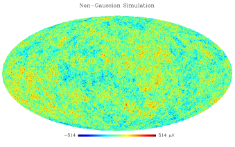
Figure 2: A realisation of a non-Gaussian all-sky CMB map with a prescribed ensemble-average power spectrum $C_{\ell}$, obtained using the non-Gaussian PDF plotted in Fig. 1 with $\alpha_{3}=0.2$, Healpix resolution parameter $N_{\mathrm{side}}=512$ (WMAP resolution) and $\ell_{\mathrm{max}}=1500$.

Figure 3: A realisation of a Gaussian all-sky CMB map drawn from the same ensemble-average power spectrum, $C_{\ell}$, as the non-Gaussian map shown in Fig. 2.

The source code to simulate the non-Gaussian CMB maps for both the full sky and for a small patch of the sky are available at the NGsims webpage.

As a guide to help the reader reproduce our method, we give here a summary of the logical steps to be taken to generate these non-Gaussian maps (see also documentation at the NGsims webpage):

1. Draw independent identically-distributed pixel values from a non-Gaussian PDF to create a statistically-isotropic map of non-Gaussian white noise;

2. Transform the map to harmonic space (with e.g. a fast spherical transform);

3. Scale the harmonic coefficients to enforce the desired power spectrum;

4. Transform back to real space to obtain a non-Gaussian map which has the desired 2-point correlation function.

We have implemented this method using two classes of non-Gaussian PDF (see documentation in NGsims webpage), but for the purposes of illustration, we adopt here PDF (i):

1. A general PDF based on the energy eigenstates of a linear harmonic oscillator, which takes the form of a Gaussian multiplied by a series of Hermite polynomials (see Appendix A). In principle this expansion can be used to generate any PDF, although if the expansion is truncated then the available values of the relative skewness are constrained.

2. The pixel values are drawn from a Gaussian distribution and then raised to some (even) integer power. This method is very fast to implement and easily generates distributions with large skewness and so is useful for checking statistical tools.

As we shall see in the next section, the simulation method described above enables one to generate non-Gaussian maps for which many of the statistical properties can be calculated analytically. The range of possible correlators and polyspectra are, however, rather restricted, with the scale dependence of the latter controlled solely by the angular power spectrum (see Section 3.2). It is, however, straightforward to extend our basic method to allow the simulation of non-Gaussian maps with a much wider range of statistical properties, as will be discussed in Section 4.

3 Statistical properties of the map

It is clear that, by construction, the non-Gaussian map plotted in Fig. 2 is statistically isotropic, with an ensemble-average power spectrum, $C_{\ell}$, corresponding to a generic inflationary cosmological model. As a check, the power spectrum of the map was calculated and found to agree with the input spectrum, as shown in Fig. 4.

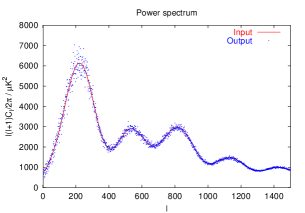
Figure 4: The power spectrum of the map shown in Fig. 2 (points) as compared with the input ensemble-average spectrum $C_{\ell}$ (solid line).

Owing to the simple manner in which the simulated non-Gaussian map is produced, many more of its statistical properties may be calculated analytically, such as the correlators of the pixel values, the bispectrum and higher-order polyspectra, and the marginalised probability distribution of the map. In this section, we again concentrate on the all-sky case; the corresponding discussion for the flat-sky approximation is given in Appendix C.

To facilitate the calculation of the statistical properties of the map, it is convenient first to express the temperature $t_{p}$ in each pixel in terms of the initial pixel values $\{s_{p}\}$ drawn from the original non-Gaussian PDF $f_{S}(s)$. Using equations (7) and (8), we begin by writing

$$t_{p} = \frac{1}{\sqrt{\mu_{2}\Omega_{\rm pix}}}\sum_{\ell,m}\sqrt{C_{\ell}}a_{\ell m}Y_{\ell m}(\textbf{{x}}_{p})$$ (9)

$$= \sqrt{\frac{\Omega_{\rm pix}}{\mu_{2}}}\sum_{p^{\prime}}s_{p^{\prime}}\sum_{\ell}\sqrt{C_{\ell}}\sum_{m}Y_{\ell m}(\textbf{{x}}_{p})Y^{*}_{\ell m}(\textbf{{x}}_{p^{\prime}}),$$

where in the second line we have substituted for $a_{\ell m}$ from equation (5). Using the spherical harmonic addition formula

$$\sum_{m}Y_{\ell m}(\textbf{{x}}_{p})Y^{*}_{\ell m}(\textbf{{x}}_{p^{\prime}})=\frac{2\ell+1}{4\pi}P_{\ell}(\textbf{{x}}_{p}\cdot\textbf{{x}}_{p^{\prime}}),$$ (10)

where $P_{\ell}(z)$ is a Legendre polynomial, we may thus write equation (9) as

$$t_{p}=\sum_{p^{\prime}}W_{pp^{\prime}}s_{p^{\prime}},$$ (11)

where the elements of the weight matrix are given by

$$W_{pp^{\prime}}=\sqrt{\frac{\Omega_{\rm pix}}{\mu_{2}}}\sum_{\ell}\frac{2\ell+1}{4\pi}\sqrt{C_{\ell}}P_{\ell}(\textbf{{x}}_{p}\cdot\textbf{{x}}_{p^{\prime}}).$$ (12)

It is also useful to express the spherical harmonic coefficients, $\bar{a}_{\ell m}$, of the map as linear superposition of the original pixel values $\{s_{p}\}$. From equations (5) and (7), we immediately obtain

$$\bar{a}_{\ell m}=\sum_{p}\widetilde{W}_{\ell m,p}s_{p},$$ (13)

where the elements of this second weight matrix are simply scaled spherical harmonics evaluated at the $p$th pixel and are given by

$$\widetilde{W}_{\ell m,p}=\sqrt{\frac{\Omega_{\rm pix}C_{\ell}}{\mu_{2}}}Y^{*}_{\ell m}(\textbf{{x}}_{p}).$$ (14)

Equations (11)–(14) provide the basic expressions from which the statistical properties of the non-Gaussian map may be obtained.

3.1 Correlators of the pixel values

Using equations (4) and (11), a general expression for the connected $n$-point correlator of the pixel values in the non-Gaussian map is given by

$$\langle t_{p_{1}}\cdots t_{p_{n}}\rangle_{c} = \sum_{q_{1}\cdots q_{n}}W_{p_{1}q_{1}}\cdots W_{p_{n}q_{n}}\langle s_{q_{1}}\cdots s_{q_{n}}\rangle_{c}$$ (15)

$$= \kappa_{n}\sum_{q}W_{p_{1}q}\cdots W_{p_{n}q},$$

where $\kappa_{n}$ is the $n$th cumulant of $f_{S}(s)$. Inserting the expression (12) into this result, we obtain

$$\langle t_{p_{1}}\cdots t_{p_{n}}\rangle_{c}=\frac{\kappa_{n}}{\Omega_{\rm pix}}\!\left(\frac{\Omega_{\rm pix}}{\mu_{2}}\right)^{n/2}\!\!\!\sum_{\ell_{1}\cdots\ell_{n}}\!\!\alpha_{\ell_{1}\cdots\ell_{n}}I_{\ell_{1}\cdots\ell_{n}}(\textbf{{x}}_{p_{1}},\ldots,\textbf{{x}}_{p_{n}}),$$ (16)

where we have defined the quantities

$$\alpha_{\ell_{1}\cdots\ell_{n}}\!\!\!\! \equiv \!\!\!\!\frac{(2\ell_{1}+1)\cdots(2\ell_{n}+1)}{(4\pi)^{n}}\sqrt{C_{\ell_{1}}\cdots C_{\ell_{n}}},$$ (17)

$$I_{\ell_{1}\cdots\ell_{n}}(\textbf{{x}}_{p_{1}},\ldots,\textbf{{x}}_{p_{n}})\!\!\!\! \equiv \!\!\!\!\sum_{q}\!P_{\ell_{1}}(\textbf{{x}}_{p_{1}}\cdot\textbf{{x}}_{q})\cdots P_{\ell_{n}}(\textbf{{x}}_{p_{n}}\cdot\textbf{{x}}_{q})\,\Omega_{\rm pix}.$$ (18)

Taking the continuum limit of the sum over $q$, we see that an analytic expression for the $n$-point correlator may be obtained by evaluating

$$I_{\ell_{1}\cdots\ell_{n}}(\textbf{{x}}_{p_{1}},\ldots,\textbf{{x}}_{p_{n}})\approx\int_{4\pi}\!\!P_{\ell_{1}}(\textbf{{x}}_{p_{1}}\cdot\textbf{{x}})\cdots P_{\ell_{n}}(\textbf{{x}}_{p_{n}}\cdot\textbf{{x}})\,\mathrm{d}\Omega.$$ (19)

Clearly, $I_{\ell_{1}\cdots\ell_{n}}$ is invariant under rigid rotations of its vector arguments, and this property is inherited by the $n$-point correlator as required by statistical isotropy. The integral may be related to the $n$-polar harmonics with zero total angular momentum (Varshalovich et al., 1988); this reduction for the first few values of $n$ is described further in Appendix B.

Using the results derived in Appendix B, one recovers, for example, the well-known result for the 2-point correlator

$$\langle t_{p_{1}}t_{p_{2}}\rangle=\sum_{\ell}\frac{2\ell+1}{4\pi}C_{\ell}P_{\ell}(\textbf{{x}}_{p_{1}}\cdot\textbf{{x}}_{p_{2}}),$$ (20)

and an explicit form for the 3-point correlator given by

$$\langle t_{p_{1}}t_{p_{2}}t_{p_{3}}\rangle_{c}$$

$$= \!\!\!\frac{\mu_{3}}{\mu_{2}^{3/2}}\Omega_{\mathrm{pix}}^{1/2}\sum_{\ell_{1},\ell_{2},\ell_{3}}\sqrt{\frac{D_{\ell_{1}}D_{\ell_{2}}D_{\ell_{3}}}{4\pi}}\left(\begin{array}[]{ccc}\ell_{1}&\ell_{2}&\ell_{3}\\ 0&0&0\end{array}\right)$$ (23)

$$\times \!\!\!\sum_{m_{1}m_{2}m_{3}}\left(\begin{array}[]{ccc}\ell_{1}&\ell_{2}&\ell_{3}\\ m_{1}&m_{2}&m_{3}\end{array}\right)Y^{*}_{\ell_{1}m_{1}}(\textbf{{x}}_{p_{1}})Y^{*}_{\ell_{2}m_{2}}(\textbf{{x}}_{p_{2}})Y^{*}_{\ell_{3}m_{3}}(\textbf{{x}}_{p_{3}}),$$ (26)

in which we have defined $D_{\ell}\equiv(2\ell+1)C_{\ell}$.

3.2 Bispectrum and higher-order polyspectra

To compute the polyspectra of the non-Gaussian map we form the $n$th connected correlator of its multipoles using equations (4) and (13):

$$\langle\bar{a}_{\ell_{1}m_{1}}\cdots\bar{a}_{\ell_{n}m_{n}}\rangle_{c} = \sum_{p_{1}\cdots p_{n}}\widetilde{W}_{\ell_{1}m_{1},p_{1}}\cdots\widetilde{W}_{\ell_{n}m_{n},p_{n}}\langle s_{p_{1}}\cdots s_{p_{n}}\rangle_{c}$$ (27)

$$= \kappa_{n}\sum_{p}\widetilde{W}_{\ell_{1}m_{1},p}\cdots\widetilde{W}_{\ell_{n}m_{n},p}.$$

Inserting the expression (14) into this result, we obtain

$$\langle\bar{a}_{\ell_{1}m_{1}}\cdots\bar{a}_{\ell_{n}m_{n}}\rangle_{c}=\frac{\kappa_{n}}{\Omega_{\rm pix}}\!\left(\frac{\Omega_{\rm pix}}{\mu_{2}}\right)^{n/2}\sqrt{C_{\ell_{1}}\cdots C_{\ell_{n}}}\,J_{\ell_{1}m_{1},\ldots,\ell_{n}m_{n}},$$ (28)

where

$$J_{\ell_{1}m_{1},\ldots,\ell_{n}m_{n}} = \sum_{p}Y^{*}_{\ell_{1}m_{1}}(\textbf{{x}}_{p})\cdots Y^{*}_{\ell_{n}m_{n}}(\textbf{{x}}_{p})\,\Omega_{\rm pix}$$ (29)

$$\approx \int_{4\pi}Y^{*}_{\ell_{1}m_{1}}(\textbf{{x}})\cdots Y^{*}_{\ell_{n}m_{n}}(\textbf{{x}})\,\mathrm{d}\Omega.$$

Integrals of this form may be reduced to products of 3$j$ symbols as discussed in Appendix B.

For the case $n=2$, one immediately recovers $\langle\bar{a}_{\ell m}\bar{a}^{*}_{\ell^{\prime}m^{\prime}}\rangle=C_{\ell}\delta_{\ell\ell^{\prime}}\delta_{mm^{\prime}}$. For $n=3$, we find that

$$\langle\bar{a}_{\ell_{1}m_{1}}\bar{a}_{\ell_{2}m_{2}}\bar{a}_{\ell_{3}m_{3}}\rangle=\left(\begin{array}[]{ccc}\ell_{1}&\ell_{2}&\ell_{3}\\ m_{1}&m_{2}&m_{3}\end{array}\right)B_{\ell_{1}\ell_{2}\ell_{3}},$$ (30)

where the bispectrum coefficients of the simulated non-Gaussian map are given by

$$B_{\ell_{1}\ell_{2}\ell_{3}}=\frac{\kappa_{3}}{\Omega_{\rm pix}}\!\left(\frac{\Omega_{\rm pix}}{\mu_{2}}\right)^{3/2}\sqrt{\frac{D_{\ell_{1}}D_{\ell_{2}}D_{\ell_{3}}}{4\pi}}\left(\begin{array}[]{ccc}\ell_{1}&\ell_{2}&\ell_{3}\\ 0&0&0\end{array}\right).$$ (31)

It is convenient also to introduce the ‘normalised’ (by the power spectrum) reduced bispectrum $\hat{b}_{\ell_{1}\ell_{2}\ell_{3}}$ by the relation

$$B_{\ell_{1}\ell_{2}\ell_{3}}=\sqrt{\frac{D_{\ell_{1}}D_{\ell_{2}}D_{\ell_{3}}}{4\pi}}\left(\begin{array}[]{ccc}\ell_{1}&\ell_{2}&\ell_{3}\\ 0&0&0\end{array}\right)\hat{b}_{\ell_{1}\ell_{2}\ell_{3}}.$$ (32)

Thus, for our simulated map, $\hat{b}_{\ell_{1}\ell_{2}\ell_{3}}$ has a constant value given by

$$\hat{b}_{\ell_{1}\ell_{2}\ell_{3}}=\frac{\kappa_{3}}{\Omega_{\rm pix}}\!\left(\frac{\Omega_{\rm pix}}{\mu_{2}}\right)^{3/2}.$$ (33)

We see that the amplitude of the bispectrum is determined by the variance $\mu_{2}$ and skewness $\kappa_{3}$ of the original non-Gaussian PDF $f_{S}(s)$. If $f_{S}(s)$ were Gaussian, for example, the bispectrum would clearly vanish. Even if $f_{S}(s)$ has a non-zero skewness, however, we note from equation (28) that, in the limit that the number of pixels tends to infinity, all polyspectra with $n\geq 3$ vanish. This is a consequence of each pixel being the weighted sum of independent identically-distributed variates, so that in the limit of an infinite number of pixels the processed map $T(\textbf{{x}})$ tends to Gaussian by the central-limit theorem. Fortunately, in practice, we can bypass this property as $N_{\mathrm{pix}}$ increases by scaling the cumulants of the initial distribution $f_{S}(s)$. For example, to get a bispectrum independent of $N_{\mathrm{pix}}$, we must scale $\kappa_{3}$ such that

$$\frac{\kappa_{3}}{\Omega_{\mathrm{pix}}}\!\left(\frac{\Omega_{\mathrm{pix}}}{\mu_{2}}\right)^{3/2}=\mbox{constant}.$$ (34)

As mentioned in Appendix A, for the particular non-Gaussian PDF used here, generating higher values of the relative skewness requires one to have a larger range of the generalized cumulants parameters $\alpha_{n}$ non zero.

As a check on our calculations, the normalised reduced bispectra of an ensemble of $300\,000$ non-Gaussian maps was calculated using an estimator defined in Spergel & Goldberg (1999) as

$$\hat{b}_{\ell_{1}\ell_{2}\ell_{3}} = \frac{1}{4\pi}\int e_{\ell_{1}}(\textbf{{x}})e_{\ell_{2}}(\textbf{{x}})e_{\ell_{3}}(\textbf{{x}})\mathrm{d}\Omega$$ (37)

$$\qquad\times\sqrt{\frac{4\pi}{D_{\ell_{1}}D_{\ell_{2}}D_{\ell_{3}}}}\left(\begin{array}[]{ccc}\ell_{1}&\ell_{2}&\ell_{3}\\ 0&0&0\end{array}\right)^{-2},$$

where, $e_{\ell}(\textbf{{x}})=\sqrt{\frac{4\pi}{2\ell+1}}\sum_{m}a_{\ell m}Y_{\ell m}(\textbf{{x}})$. The resulting mean values of $\hat{b}_{\ell\ell\ell}$ are plotted in Fig. 5, together with the associated uncertainties. Note that it is important to divide the measured bispectrum by the ensemble-averaged values of the power spectrum; dividing by the measured values for each simulation produces a biased estimator.

Figure 5: Non-zero diagonal components of the bispectrum estimated from $300\,000$ non-Gaussian simulations with the same parameters as those used in Fig. 2. The mean over the simulations and its standard error are plotted. The dashed line is the theoretical ensemble-average value. Note that the diagonal bispectrum necessarily vanishes for odd $\ell$ by parity.

The predicted value of $\hat{b}_{\ell_{1}\ell_{2}\ell_{3}}$ was calculated using (33) and is plotted as the solid line in the figure. We see that the measured and predicted values are fully consistent.

Returning to equation (28), if one considers $n=4$ and follows the notation of Hu (2001), one finds that the connected part of the trispectrum of the non-Gaussian simulation is given by

$$T_{\ell_{3}\ell_{4}}^{\ell_{1}\ell_{2}}(L) = \frac{\Omega_{\mathrm{pix}}\kappa_{4}}{\mu_{2}^{2}}\sqrt{D_{\ell_{1}}D_{\ell_{2}}D_{\ell_{3}}D_{\ell_{4}}}\frac{2L+1}{4\pi}$$ (42)

$$\qquad\times\left(\begin{array}[]{ccc}\ell_{1}&\ell_{2}&L\\ 0&0&0\end{array}\right)\left(\begin{array}[]{ccc}\ell_{3}&\ell_{4}&L\\ 0&0&0\end{array}\right).$$

Analytic expressions for higher-order polyspectra may be obtained in an analogous manner.

3.3 Cumulants and marginal distribution

Finally, we consider the marginal PDF $f_{T}(t)$ of the processed map. This is mostly easily carried out by considering the cumulants of $f_{T}(t)$, and relating them to those of the original non-Gaussian PDF $f_{S}(s)$.

The cumulants of the marginal PDF are equal to the connected parts of the correlators of the pixel temperatures with all pixels in the correlator the same. From equation (15), we find that

$$\kappa^{\prime}_{n} = \left(\sum_{p^{\prime}}^{N_{\mathrm{pix}}}W^{n}_{pp^{\prime}}\right)\kappa_{n}$$ (43)

$$= \frac{\kappa_{n}}{\Omega_{\mathrm{pix}}}\left(\frac{\Omega_{\mathrm{pix}}}{\mu_{2}}\right)^{n/2}\sum_{\ell_{1}\cdots\ell_{n}}\alpha_{\ell_{1}\cdots\ell_{n}}I_{\ell_{1}\cdots\ell_{n}}(\textbf{{x}}_{p},\ldots,\textbf{{x}}_{p}),$$

which is independent of the choice of pixel $p$. Evaluating the rotationally-invariant function $I_{\ell_{1}\cdots\ell_{n}}(\textbf{{x}}_{p},\ldots,\textbf{{x}}_{p})$ along the polar axis, where $Y_{\ell m}(\hat{\textbf{{z}}})=\sqrt{(2l+1)/4\pi}\delta_{m0}$, we find that the first few cumulants (beyond $\kappa^{\prime}_{1}=0$) are

$$\kappa^{\prime}_{2}\!\!\!\! = \!\!\!\!\sum_{\ell}\frac{2\ell+1}{4\pi}C_{\ell}$$

$$\kappa^{\prime}_{3}\!\!\!\! = \!\!\!\!\sum_{\ell_{1}\ell_{2}\ell_{3}}B_{\ell_{1}\ell_{2}\ell_{3}}\sqrt{\frac{2\ell_{1}+1}{4\pi}\cdots\frac{2\ell_{3}+1}{4\pi}}\left(\begin{array}[]{ccc}\ell_{1}&\ell_{2}&\ell_{3}\\ 0&0&0\end{array}\right)$$

$$\kappa^{\prime}_{4}\!\!\!\! = \!\!\!\!\sum_{\ell_{1}\cdots\ell_{4}}\sqrt{\frac{2\ell_{1}+1}{4\pi}\cdots\frac{2\ell_{4}+1}{4\pi}}$$

$$\qquad\times\sum_{L}T_{\ell_{3}\ell_{4}}^{\ell_{1}\ell_{2}}(L)\left(\begin{array}[]{ccc}\ell_{1}&\ell_{2}&L\\ 0&0&0\end{array}\right)\left(\begin{array}[]{ccc}\ell_{3}&\ell_{4}&L\\ 0&0&0\end{array}\right),$$

where we have written the results in such as way that they are true generally, for any statistically-isotropic map.

In principle, knowledge of the complete set of cumulants $\kappa^{\prime}_{n}$ may be used to obtain an explicit expression for the marginal PDF $f_{T}(t)$. This could be carried out, for example, by first obtaining its moment-generating function

$$M_{T}(k)=\langle\mathrm{e}^{\mathrm{i}kt}\rangle=\exp\left(\sum_{n=1}^{\infty}\frac{(\mathrm{i}k)^{n}}{n!}\kappa^{\prime}_{n}\right),$$ (46)

and then performing an inverse Fourier transform to yield $f_{T}(t)$. Alternatively, for a weakly non-Gaussian distribution, one can employ the Edgeworth expansion. In this approach, the PDF is expressed as an asymptotic expansion around a Gaussian with mean zero and variance $\sigma^{2}=\kappa^{\prime}_{2}$ to yield

$$f_{T}(t) \approx \frac{\mathrm{e}^{-\hat{t}^{2}}}{\sqrt{2\pi\sigma^{2}}}\Bigl{(}1+\frac{\kappa^{\prime}_{3}/\sigma^{3}}{12\sqrt{2}}H_{3}(\hat{t})+\frac{\kappa^{\prime}_{4}/\sigma^{4}}{96}H_{4}(\hat{t})$$ (47)

$$+\frac{\kappa^{\prime}_{5}/\sigma^{5}}{480\sqrt{2}}H_{5}(\hat{t})+\frac{(\kappa^{\prime}_{6}+10{\kappa^{\prime}_{3}}^{2})/\sigma^{6}}{5760}H_{6}(\hat{t})+\cdots\Bigr{)},$$

where $\hat{t}=t/\sqrt{2}\sigma$. When $\kappa^{\prime}_{n}/\sigma^{n}$ is small for $n$ larger than some integer one can use a finite number of cumulants as an acceptable approximation to the distribution. As pointed out by Rocha et al. (2001), however, this might no longer be a PDF and, in particular, might deviate from the original distribution in the tails. In Fig.6 we plot the histogram of the pixel temperatures for a non-Gaussian map with $N_{\mathrm{side}}=64$ and $\ell_{\mathrm{max}}=128$ (somewhat lower resolution than that plotted in Fig. 2), generated from an initial PDF with parameters $\alpha_{3}=0.27$ and $\sigma_{0}=1$. Overplotted is the Edgeworth expansion of $f_{T}(t)$, equation (47), truncated at $n=4$. The cumulants of $f_{T}(t)$ can be computed efficiently from the first expression in equation (43); we find $\kappa^{\prime}_{1}=0$, $\kappa^{\prime}_{2}\approx 13809\,{\mu\mathrm{K}}^{2}$, $\kappa^{\prime}_{3}\approx 177234\,{\mu\mathrm{K}}^{3}$ and $\kappa^{\prime}_{4}\approx 6307963\,{\mu\mathrm{K}}^{4}$. The Edgeworth expansion agrees with the simulation results better than a Gaussian with the same variance.

Figure 6: Histogram of pixel temperatures for the final processed non-Gaussian map for $N_{side}=64$ and $\ell_{\mathrm{max}}=128$, created using an initial PDF with parameters $\alpha_{3}=0.27$ and $\sigma_{0}=1$. Also shown are the Edgeworth expansion for $f_{T}(t)$ (dashed line), given by equation (47) but truncated at $n=4$, and a Gaussian with the same variance (solid line).

4 Extended simulation method

We see from the previous section that our basic simulation method generates maps with a rather restricted range of possible correlators and polyspectra, with the scale dependence of the latter controlled solely by the angular power spectrum. It is straightforward, however, to extend our basic method to allow the simulation of non-Gaussian maps with a much wider range of statistical properties. In particular, there is no fundamental requirement for the method to be restricted to the same set of cumulants over the whole range of scales.

The procedure is as follows. One divides the range of multipoles, $\ell$, into non-overlapping bins. A given bin $B$ will be a set $B=[\ell_{B_{\mathrm{min}}},\ell_{B_{\mathrm{max}}}]$. For each bin $B$ we simulate a map $t_{Bp}$, with non-zero $C_{\ell}$ only for $\ell\in B$ and a non-Gaussian PDF that can differ between bins. The final map is a superposition of these band maps, i.e. with pixel values

$$t_{p}=\sum_{B}t_{Bp}.$$ (48)

Since each map $t_{Bp}$ is individually statistically isotropic, then so too is their sum. Moreover, from equation (32), we see that the bispectrum for each band map can only be non-zero within the corresponding bin (this is also true for the connected parts of higher-order polyspectra). The $n$th cumulant of the final map is also simply the sum of the $n$th cumulants of the individual band maps. With this method we are thus able to generate maps with more general statistical properties.

For example, by choosing appropriate values of $\kappa_{3}$ for the non-Gaussian PDF used to simulate each band map, one can arrange for the summed map (48) to have a given power spectrum $C_{\ell}$ and an arbitrary prescribed constant value of the reduced normalised bispectrum $\hat{b}_{\ell_{1}\ell_{2}\ell_{3}}$ in each bin. As an illustration, in Fig. 7 we plot a non-Gaussian map generated using three bins. In each bin, the non-Gaussian PDF used was of the form given in equation (51) with $\sigma_{0}=1$. However, the values of $\alpha_{3}$ used in each bin were $\alpha_{3}=0.1$, $0.2$ and $0.25$ respectively.

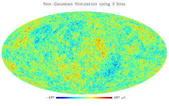
Figure 7: A realisation of a non-Gaussian all-sky map simulation using three bins: $B_{1}=[0,500],\alpha_{3}=0.1$; $B_{2}=[501,1000],\alpha_{3}=0.2$; and $B_{3}=[1001,1500],\alpha_{3}=0.25$.

As a check on our calculations, the normalised reduced bispectrum of an ensemble of $300\,000$ such non-Gaussian maps was calculated using the estimator (37). The resulting mean values of $\hat{b}_{\ell\ell\ell}$, for individual values of $\ell$, are plotted in Fig. 8, together with the associated uncertainties. The predicted value of $\hat{b}_{\ell\ell\ell}$ in each of the three broad bins was calculated using equation (33) and are plotted as the dashed lines in the figure. We see that once again the measured and predicted values are fully consistent.

Figure 8: Non-zero diagonal components of the bispectrum estimated from $300\,000$ non-Gaussian simulations using three bins: $B_{1}=[0,21],\alpha_{3}=0.1$; $B_{2}=[22,43],\alpha_{3}=0.2$; and $B_{3}=[44,56],\alpha_{3}=0.25$. The mean over the simulations and its standard error are plotted. The dashed lines shows the theoretical ensemble-average value in each bin.

How general is our extended method? We can in principle efficiently generate maps with arbitrary diagonal bispectra, i.e. with any given $C_{\ell}$ and $B_{\ell\ell\ell}$. This is of some importance because currently known primordial theories of non-Gaussianity lead to more general combinations of angular power spectra and bispectra than can be created from our method with a single univariate PDF $f_{S}(s)$. It is not possible, however, to generate specific models of primordial non-Gaussianity exactly with our extended method. To do that one would have to be able to choose arbitrary values for the angular spectrum and for all components of the bispectrum (and higher polyspectra). This would involve going beyond the simple one-point PDF methods advocated here.

5 Conclusions

We presented a simple, fast method for simulating statistically-isotropic non-Gaussian CMB maps with a given power spectrum and analytically calculable bispectrum. We showed that our technique allows one to describe the statistical properties of the map by computing analytically the $n$th-order polyspectra, and the $n$th-order correlators of the pixel values. We showed that these can be expressed in terms of the $n$-polar harmonics with zero total angular momentum, and we describe this reduction for the first few values of $n$. We also recovered analytically the one-dimensional marginalised distribution function in terms of its cumulants. The univariate non-Gaussian distribution, from which the pixel values are drawn independently in the first stage of the simulation process, fully determines the statistical properties of the final map. Here we used a non-Gaussian distribution derived from the wavefunctions of the harmonic oscillator. Simulations of both the full sky and a small patch of the sky were generated and corresponding statistical analysis performed. As a check on our calculations we computed both the power spectrum and bispectrum of the simulated maps and found them to be fully consistent. The simulation method described here clearly enables one to generate maps with well-defined correlators and polyspectra. We extended the method to encompass different set of cumulants over the whole range of scales, generating maps with arbitrary power spectra and diagonal bispectra for different scales. It is not possible, however, to generate specific models of primordial non-Gaussianity exactly with our extended method, since these require off-diagonal bispectrum coefficients to be specified arbitrarily. This would involve going beyond the simple one-point PDF methods advocated here.

The source code to simulate the non-Gaussian CMB maps for both the full sky and for a small patch of the sky are available at the NGsims webpage.

A pertinent question is what other statistical properties can be calculated analytically for the class of non-Gaussian maps we have investigated. Of particular interest are the phase associations between different harmonic coefficients. In Matsubara (2003), a general relationship between phase correlations and the hierarchy of polyspectra in Fourier space is established. It is also stated that the phase correlations are related to the polyspectra through the non-uniform distribution of the phase sum $\theta_{\textbf{{k}}_{1}}+\theta_{\textbf{{k}}_{2}}+\cdots+\theta_{\textbf{{k}}_{N}}$ with closed vectors $\textbf{{k}}_{1}+\textbf{{k}}_{2}+\cdots+\textbf{{k}}_{N}=\textbf{{0}}$. We are currently investigating the form of the distribution function of this phase sum in our maps. A study of the Minkowski functionals of our non-Gaussian maps is also underway.

6 Ackowledgements

We thank Carlo Contaldi and Neil Turok for useful discussions, and Martin Kunz and Grazia De Troia for providing us with the bispectrum code for the full-sky case. Some of the results in this paper have been derived using the Healpix (Gorski, Hivon, and Wandelt 1999) package. GR acknowledges a Leverhulme Fellowship at the University of Cambridge. PF and AC acknowledge Royal Society University Research Fellowships. SS acknowledges support by a PPARC studentship.

Appendix A Non-Gaussian PDFs based on the harmonic oscillator

In this appendix, we summarise the class of probability distribution functions (PDFs) derived from the Hilbert space of a linear harmonic oscillator, which was developed by Rocha et al. (2001). The original non-Gaussian distribution, $f_{S}(s)$, used in the main text to produce the simulated non-Gaussian maps is an example of such a PDF.

This general PDF is based on the coordinate-space wavefunctions of the energy eigenstates of a linear harmonic oscillator, and takes the form of a Gaussian multiplied by the square of a (possibly finite) series of Hermite polynomials whose coefficients $\alpha_{n}$ are used as non-Gaussian qualifiers. In particular, if $x$ is a general random variable, the most general PDF has the form

$$p(x)=|\psi|^{2}=\mathrm{e}^{-x^{2}/(2\sigma_{0}^{2})}\left|\sum_{n}\alpha_{n}C_{n}H_{n}{\left(x\over{\sqrt{2}}\sigma_{0}\right)}\right|^{2},$$ (49)

where $H_{n}(x)$ are the Hermite polynomials, and the quantity $\sigma_{0}^{2}$ is the variance associated with the (Gaussian) probability distribution for the ground state $|\psi_{0}|^{2}$. The constants $C_{n}$ are fixed by normalising the individual states. The only constraint upon the amplitudes $\alpha_{n}$ is

$$\sum|\alpha_{n}|^{2}=1.$$ (50)

This is a simple algebraic expression which can be eliminated explicitly by writing $\alpha_{0}=\sqrt{1-\sum_{1}^{\infty}|\alpha_{n}|^{2}}$. Thus the coefficients $\alpha_{n}$ can be independently set to zero without mathematical inconsistency (Rocha et al., 2001). Moreover, these coefficients can be written as series of cumulants (Contaldi, Bean & Magueijo, 1999) and should indeed be regarded as non-perturbative generalisations of cumulants.

For the simulations in the main text, we use the non-Gaussian PDF for which all $\alpha_{n}$ are set to zero, except for the real part of $\alpha_{3}$ (and consequently $\alpha_{0}$). The reason for this choice is that this quantity reduces to the skewness in the perturbative regime. The imaginary part of $\alpha_{3}$ is only meaningful in the non-perturbative regime (and can be set to zero independently without inconsistency). Hence we consider a PDF of the form

$$p(x)=\frac{\mathrm{e}^{-x^{2}/(2\sigma_{0}^{2})}}{\sqrt{2\pi}\sigma_{0}}\left[\alpha_{0}+\frac{\alpha_{3}}{\sqrt{48}}H_{3}\left(\frac{x}{\sqrt{2}\sigma_{0}}\right)\right]^{2},$$ (51)

with $\alpha_{0}=\sqrt{1-\alpha_{3}^{2}}$. It is straightforward to show that the first, second and third moments of our PDF are related to $\alpha_{3}$ and $\sigma_{0}$ by (Contaldi & Magueijo, 2001)

$$\mu_{1} = 0$$

$$\mu_{2} = \sigma_{0}^{2}\left(1+6\alpha_{3}^{2}\right)$$

$$\mu_{3} = \left(2\sigma_{0}^{2}\right)^{\frac{3}{2}}\sqrt{3\left[\alpha_{3}^{2}\left(1-\alpha_{3}^{2}\right)\right]}.$$ (52)

The PDF therefore has zero mean and a fixed variance and skewness. In the simulations discussed in the main text, we choose $\alpha_{3}=0.2$ and $\sigma_{0}=1$. This resulting PDF is plotted in Fig. 1.

We note that the space of possible PDFs is constrained as a result of restricting the set of coefficients $\alpha_{n}$ to two non-zero values. This implies that we cannot generate distributions with arbitrarily large relative skewness. Indeed, $\mu_{3}/\mu_{2}^{3/2}$ is bounded above by 0.74, and takes this maximum value for $\alpha_{3}^{2}=(7-\sqrt{43})/6=0.27^{2}$. However, in general our method can generate higher values of the relative skewness (since it can generate any distribution) but for that purpose one needs more non-zero coefficients $\alpha_{n}$ (Contaldi & Magueijo, 2001).

Appendix B Some useful integrals

We give here useful results concerning integrals involving products of Legendre polynomials:

$$I_{\ell_{1}\cdots\ell_{n}}(\textbf{{x}}_{1},\ldots,\textbf{{x}}_{n})\equiv\int_{4\pi}\!\!P_{\ell_{1}}(\textbf{{x}}_{1}\cdot\textbf{{x}})\cdots P_{\ell_{n}}(\textbf{{x}}_{n}\cdot\textbf{{x}})\,\mathrm{d}\Omega.$$ (53)

Using the addition theorem (equation 10), this reduces to evaluating integrals of products of spherical harmonics,

$$J_{\ell_{1}m_{1},\ldots,\ell_{n}m_{n}}\equiv\int_{4\pi}\!\!Y_{\ell_{1}m_{1}}(\textbf{{x}})\cdots Y_{\ell_{n}m_{n}}(\textbf{{x}})\,\mathrm{d}\Omega$$ (54)

since

$$I_{\ell_{1},\cdots,\ell_{n}}(\textbf{{x}}_{1},\ldots,\textbf{{x}}_{n})=\frac{4\pi}{2\ell_{1}+1}\cdots\frac{4\pi}{2\ell_{n}+1}\sum_{m_{1}\cdots m_{n}}Y^{*}_{\ell_{1}m_{1}}(\textbf{{x}}_{1})\cdots Y^{*}_{\ell_{n}m_{n}}(\textbf{{x}}_{n})J_{\ell_{1}m_{1},\ldots,\ell_{n}m_{n}}.$$ (55)

First, consider the case $n=2$. Using the orthonormality of the spherical harmonics, and the relation $Y_{\ell m}^{*}(\textbf{{x}})=(-1)^{m}Y_{\ell-m}(\textbf{{x}})$, to evaluate $J_{\ell_{1}m_{1},\ell_{2}m_{2}}=(-1)^{m_{1}}\delta_{\ell_{1}\ell_{2}}\delta_{m_{1}\,-m_{2}}$, and then applying the addition theorem we find the well-known result

$$I_{\ell_{1}\ell_{2}}(\textbf{{x}}_{1},\textbf{{x}}_{2})=\frac{4\pi}{2\ell_{1}+1}P_{\ell_{1}}(\textbf{{x}}_{1}\cdot\textbf{{x}}_{2})\delta_{\ell_{1}\ell_{2}}.$$ (56)

For integrals involving products of three or more spherical harmonics, the general strategy is to combine pairs of harmonics using the Clebsch-Gordan series (e.g. Varshalovich et al. 1988; Edmonds 1974)

$$Y_{\ell_{1}m_{1}}(\textbf{{x}})Y_{\ell_{2}m_{2}}(\textbf{{x}})=\sum_{\ell m}\sqrt{\frac{(2\ell_{1}+1)(2\ell_{2}+1)(2\ell+1)}{4\pi}}\left(\begin{array}[]{ccc}\ell_{1}&\ell_{2}&\ell\\ m_{1}&m_{2}&m\end{array}\right)\left(\begin{array}[]{ccc}\ell_{1}&\ell_{2}&\ell\\ 0&0&0\end{array}\right)Y^{*}_{\ell m}(\textbf{{x}}),$$ (57)

until we have only a single pair left which can then be integrated trivially using orthonormality. We illustrate this procedure for the case of $n=3$ and $n=4$ since these are needed for the calculation of the bispectrum and trispectrum. For $n=3$, from equation (57) we find immediately that

$$J_{\ell_{1}m_{1},\ldots,\ell_{3}m_{3}}=\sqrt{\frac{(2\ell_{1}+1)(2\ell_{2}+1)(2\ell_{3}+1)}{4\pi}}\left(\begin{array}[]{ccc}\ell_{1}&\ell_{2}&\ell_{3}\\ 0&0&0\end{array}\right)\left(\begin{array}[]{ccc}\ell_{1}&\ell_{2}&\ell_{3}\\ m_{1}&m_{2}&m_{3}\end{array}\right),$$ (58)

and therefore

$$I_{\ell_{1}\ell_{2}\ell_{3}}(\textbf{{x}}_{1},\textbf{{x}}_{2},\textbf{{x}}_{3})=(4\pi)^{2}\sqrt{\frac{4\pi}{(2\ell_{1}+1)(2\ell_{2}+1)(2\ell_{3}+1)}}\left(\begin{array}[]{ccc}\ell_{1}&\ell_{2}&\ell_{3}\\ 0&0&0\end{array}\right)\sum_{m_{1}m_{2}m_{3}}\left(\begin{array}[]{ccc}\ell_{1}&\ell_{2}&\ell_{3}\\ m_{1}&m_{2}&m_{3}\end{array}\right)Y^{*}_{\ell_{1}m_{1}}(\textbf{{x}}_{1})Y^{*}_{\ell_{2}m_{2}}(\textbf{{x}}_{2})Y^{*}_{\ell_{3}m_{3}}(\textbf{{x}}_{3}).$$ (59)

The final term in this equation (the summation over $m_{1}$, $m_{2}$ and $m_{3}$) ensures that $I_{\ell_{1}\ell_{2}\ell_{3}}$ is invariant under rigid rotations of its vector arguments $\textbf{{x}}_{1}$, $\textbf{{x}}_{2}$ and $\textbf{{x}}_{3}$. As expected, the summation can be expressed in terms of the tripolar spherical harmonics with zero total angular momentum (Varshalovich et al., 1988).

Consider now the case $n=4$. There is now some freedom in the choice of spherical harmonics to combine. If we couple $Y_{\ell_{1}m_{1}}$ with $Y_{\ell_{2}m_{2}}$ and $Y_{\ell_{3}m_{3}}$ with $Y_{\ell_{4}m_{4}}$, we find

$$J_{\ell_{1}m_{1},\ldots,\ell_{4}m_{4}} = \sum_{\ell m}(-1)^{m}\sqrt{\frac{(2\ell_{1}+1)(2\ell_{2}+1)(2\ell+1)}{4\pi}}\sqrt{\frac{(2\ell_{3}+1)(2\ell_{4}+1)(2\ell+1)}{4\pi}}$$ (69)

$$\qquad\times\left(\begin{array}[]{ccc}\ell_{1}&\ell_{2}&\ell\\ m_{1}&m_{2}&m\end{array}\right)\left(\begin{array}[]{ccc}\ell_{3}&\ell_{4}&\ell\\ m_{3}&m_{4}&-m\end{array}\right)\left(\begin{array}[]{ccc}\ell_{1}&\ell_{2}&\ell\\ 0&0&0\end{array}\right)\left(\begin{array}[]{ccc}\ell_{3}&\ell_{4}&\ell\\ 0&0&0\end{array}\right).$$

The expression on the right is not manifestly symmetric with respect to interchange of e.g. $(\ell_{1}m_{1})$ and $(\ell_{3}m_{3})$ since the latter involves a different coupling scheme. However, the symmetry is easily verified by switching between the two schemes with the 6$j$ coefficients (Varshalovich et al., 1988). Finally, we find that

$$I_{\ell_{1}\cdots\ell_{4}}(\textbf{{x}}_{1},\ldots,\textbf{{x}}_{4}) = (4\pi)^{3/2}\sqrt{\frac{(2\ell_{1}+1)\cdots(2\ell_{4}+1)}{4\pi}}\sum_{l}\frac{2l+1}{4\pi}\left(\begin{array}[]{ccc}\ell_{1}&\ell_{2}&\ell\\ 0&0&0\end{array}\right)\left(\begin{array}[]{ccc}\ell_{3}&\ell_{4}&\ell\\ 0&0&0\end{array}\right)$$ (79)

$$\mbox{}\times\sum_{mm_{1}\cdots m_{4}}(-1)^{m}\left(\begin{array}[]{ccc}\ell_{1}&\ell_{2}&\ell\\ m_{1}&m_{2}&m\end{array}\right)\left(\begin{array}[]{ccc}\ell_{3}&\ell_{4}&\ell\\ m_{3}&m_{4}&-m\end{array}\right)Y_{\ell_{1}m_{1}}^{*}(\textbf{{x}}_{1})Y_{\ell_{2}m_{2}}^{*}(\textbf{{x}}_{2})Y_{\ell_{3}m_{3}}^{*}(\textbf{{x}}_{3})Y_{\ell_{4}m_{4}}^{*}(\textbf{{x}}_{4}).$$

It is straightforward to verify that the last term on the right (the summation over $m$, $m_{1},\ldots,m_{4}$) is invariant under rigid rotations of $\textbf{{x}}_{1},\ldots,\textbf{{x}}_{4}$.

Appendix C Flat-Sky Approximation

For analysis over a small patch of the sky we can use the flat-sky approximation and replace spherical transforms by Fourier transforms. Our starting point is again a pixelised map of non-Gaussian white noise, with each pixel value drawn from the non-Gaussian PDF $f_{S}(s)$. Approximating the Fourier transform $a(\kern-0.20004pt\hbox{$\ell$}\kern-4.16669pt\kern 0.39993pt\hbox{$\ell$}\kern-4.16669pt\kern-0.20004pt\hbox{$\ell$}\kern-4.16669pt\raise 0.20004pt\hbox{$\ell$}\kern-4.16669pt\raise-0.20004pt\hbox{$\ell$})$ by a discrete Fourier transform we have

$$a(\kern-0.20004pt\hbox{$\ell$}\kern-4.16669pt\kern 0.39993pt\hbox{$\ell$}\kern-4.16669pt\kern-0.20004pt\hbox{$\ell$}\kern-4.16669pt\raise 0.20004pt\hbox{$\ell$}\kern-4.16669pt\raise-0.20004pt\hbox{$\ell$})=\int\frac{\mathrm{d}^{2}\textbf{{x}}}{2\pi}\,S(\textbf{{x}})\mathrm{e}^{-\mathrm{i}\kern-0.14003pt\hbox{$\ell$}\kern-2.91669pt\kern 0.27995pt\hbox{$\ell$}\kern-2.91669pt\kern-0.14003pt\hbox{$\ell$}\kern-2.91669pt\raise 0.14003pt\hbox{$\ell$}\kern-2.91669pt\raise-0.14003pt\hbox{$\ell$}\cdot\textbf{{x}}}\approx\frac{\Omega_{\mathrm{pix}}}{2\pi}\sum_{p}s_{p}\mathrm{e}^{-\mathrm{i}\kern-0.14003pt\hbox{$\ell$}\kern-2.91669pt\kern 0.27995pt\hbox{$\ell$}\kern-2.91669pt\kern-0.14003pt\hbox{$\ell$}\kern-2.91669pt\raise 0.14003pt\hbox{$\ell$}\kern-2.91669pt\raise-0.14003pt\hbox{$\ell$}\cdot\textbf{{x}}_{p}},$$ (80)

where $\Omega_{\mathrm{pix}}$ is the pixel area. We evaluate $a(\kern-0.20004pt\hbox{$\ell$}\kern-4.16669pt\kern 0.39993pt\hbox{$\ell$}\kern-4.16669pt\kern-0.20004pt\hbox{$\ell$}\kern-4.16669pt\raise 0.20004pt\hbox{$\ell$}\kern-4.16669pt\raise-0.20004pt\hbox{$\ell$})$ on a regular grid in Fourier space with a Fast Fourier Transform. For a square patch of sky with $N_{\mathrm{pix}}$ pixels, the cell size in Fourier space is $(2\pi)^{2}/(N_{\mathrm{pix}}\Omega_{\mathrm{pix}})$. The second-order correlator of the discrete $a(\kern-0.20004pt\hbox{$\ell$}\kern-4.16669pt\kern 0.39993pt\hbox{$\ell$}\kern-4.16669pt\kern-0.20004pt\hbox{$\ell$}\kern-4.16669pt\raise 0.20004pt\hbox{$\ell$}\kern-4.16669pt\raise-0.20004pt\hbox{$\ell$})$ evaluates to

$$\langle a(\kern-0.20004pt\hbox{$\ell$}\kern-4.16669pt\kern 0.39993pt\hbox{$\ell$}\kern-4.16669pt\kern-0.20004pt\hbox{$\ell$}\kern-4.16669pt\raise 0.20004pt\hbox{$\ell$}\kern-4.16669pt\raise-0.20004pt\hbox{$\ell$})a^{*}(\kern-0.20004pt\hbox{$\ell$}\kern-4.16669pt\kern 0.39993pt\hbox{$\ell$}\kern-4.16669pt\kern-0.20004pt\hbox{$\ell$}\kern-4.16669pt\raise 0.20004pt\hbox{$\ell$}\kern-4.16669pt\raise-0.20004pt\hbox{$\ell$}^{\prime})\rangle=\left(\frac{\Omega_{\mathrm{pix}}}{2\pi}\right)^{2}N_{\mathrm{pix}}\mu_{2}\delta_{\kern-0.14003pt\hbox{$\ell$}\kern-2.91669pt\kern 0.27995pt\hbox{$\ell$}\kern-2.91669pt\kern-0.14003pt\hbox{$\ell$}\kern-2.91669pt\raise 0.14003pt\hbox{$\ell$}\kern-2.91669pt\raise-0.14003pt\hbox{$\ell$}\kern-0.14003pt\hbox{$\ell$}\kern-2.91669pt\kern 0.27995pt\hbox{$\ell$}\kern-2.91669pt\kern-0.14003pt\hbox{$\ell$}\kern-2.91669pt\raise 0.14003pt\hbox{$\ell$}\kern-2.91669pt\raise-0.14003pt\hbox{$\ell$}^{\prime}},$$ (81)

where $\mu_{2}$ is the variance of the zero-mean $f_{S}(s)$. In the continuum limit, equation (81) becomes

$$\langle a(\kern-0.20004pt\hbox{$\ell$}\kern-4.16669pt\kern 0.39993pt\hbox{$\ell$}\kern-4.16669pt\kern-0.20004pt\hbox{$\ell$}\kern-4.16669pt\raise 0.20004pt\hbox{$\ell$}\kern-4.16669pt\raise-0.20004pt\hbox{$\ell$})a^{*}(\kern-0.20004pt\hbox{$\ell$}\kern-4.16669pt\kern 0.39993pt\hbox{$\ell$}\kern-4.16669pt\kern-0.20004pt\hbox{$\ell$}\kern-4.16669pt\raise 0.20004pt\hbox{$\ell$}\kern-4.16669pt\raise-0.20004pt\hbox{$\ell$}^{\prime})\rangle=\Omega_{\mathrm{pix}}\mu_{2}\delta(\kern-0.20004pt\hbox{$\ell$}\kern-4.16669pt\kern 0.39993pt\hbox{$\ell$}\kern-4.16669pt\kern-0.20004pt\hbox{$\ell$}\kern-4.16669pt\raise 0.20004pt\hbox{$\ell$}\kern-4.16669pt\raise-0.20004pt\hbox{$\ell$}-\kern-0.20004pt\hbox{$\ell$}\kern-4.16669pt\kern 0.39993pt\hbox{$\ell$}\kern-4.16669pt\kern-0.20004pt\hbox{$\ell$}\kern-4.16669pt\raise 0.20004pt\hbox{$\ell$}\kern-4.16669pt\raise-0.20004pt\hbox{$\ell$}^{\prime}),$$ (82)

where we have used

$$\delta_{\kern-0.14003pt\hbox{$\ell$}\kern-2.91669pt\kern 0.27995pt\hbox{$\ell$}\kern-2.91669pt\kern-0.14003pt\hbox{$\ell$}\kern-2.91669pt\raise 0.14003pt\hbox{$\ell$}\kern-2.91669pt\raise-0.14003pt\hbox{$\ell$}\kern-0.14003pt\hbox{$\ell$}\kern-2.91669pt\kern 0.27995pt\hbox{$\ell$}\kern-2.91669pt\kern-0.14003pt\hbox{$\ell$}\kern-2.91669pt\raise 0.14003pt\hbox{$\ell$}\kern-2.91669pt\raise-0.14003pt\hbox{$\ell$}^{\prime}}=\frac{1}{N_{\mathrm{pix}}}\sum_{p}\mathrm{e}^{\mathrm{i}(\kern-0.14003pt\hbox{$\ell$}\kern-2.91669pt\kern 0.27995pt\hbox{$\ell$}\kern-2.91669pt\kern-0.14003pt\hbox{$\ell$}\kern-2.91669pt\raise 0.14003pt\hbox{$\ell$}\kern-2.91669pt\raise-0.14003pt\hbox{$\ell$}-\kern-0.14003pt\hbox{$\ell$}\kern-2.91669pt\kern 0.27995pt\hbox{$\ell$}\kern-2.91669pt\kern-0.14003pt\hbox{$\ell$}\kern-2.91669pt\raise 0.14003pt\hbox{$\ell$}\kern-2.91669pt\raise-0.14003pt\hbox{$\ell$}^{\prime})\cdot\textbf{{x}}_{p}}\rightarrow\frac{1}{N_{\mathrm{pix}}\Omega_{\mathrm{pix}}}\int\mathrm{d}^{2}\textbf{{x}}\,\mathrm{e}^{\mathrm{i}(\kern-0.14003pt\hbox{$\ell$}\kern-2.91669pt\kern 0.27995pt\hbox{$\ell$}\kern-2.91669pt\kern-0.14003pt\hbox{$\ell$}\kern-2.91669pt\raise 0.14003pt\hbox{$\ell$}\kern-2.91669pt\raise-0.14003pt\hbox{$\ell$}-\kern-0.14003pt\hbox{$\ell$}\kern-2.91669pt\kern 0.27995pt\hbox{$\ell$}\kern-2.91669pt\kern-0.14003pt\hbox{$\ell$}\kern-2.91669pt\raise 0.14003pt\hbox{$\ell$}\kern-2.91669pt\raise-0.14003pt\hbox{$\ell$}^{\prime})\cdot\textbf{{x}}}=\frac{(2\pi)^{2}}{N_{\mathrm{pix}}\Omega_{\mathrm{pix}}}\delta(\kern-0.20004pt\hbox{$\ell$}\kern-4.16669pt\kern 0.39993pt\hbox{$\ell$}\kern-4.16669pt\kern-0.20004pt\hbox{$\ell$}\kern-4.16669pt\raise 0.20004pt\hbox{$\ell$}\kern-4.16669pt\raise-0.20004pt\hbox{$\ell$}-\kern-0.20004pt\hbox{$\ell$}\kern-4.16669pt\kern 0.39993pt\hbox{$\ell$}\kern-4.16669pt\kern-0.20004pt\hbox{$\ell$}\kern-4.16669pt\raise 0.20004pt\hbox{$\ell$}\kern-4.16669pt\raise-0.20004pt\hbox{$\ell$}^{\prime}).$$ (83)

We scale the $a(\kern-0.20004pt\hbox{$\ell$}\kern-4.16669pt\kern 0.39993pt\hbox{$\ell$}\kern-4.16669pt\kern-0.20004pt\hbox{$\ell$}\kern-4.16669pt\raise 0.20004pt\hbox{$\ell$}\kern-4.16669pt\raise-0.20004pt\hbox{$\ell$})$ defining $\bar{a}(\kern-0.20004pt\hbox{$\ell$}\kern-4.16669pt\kern 0.39993pt\hbox{$\ell$}\kern-4.16669pt\kern-0.20004pt\hbox{$\ell$}\kern-4.16669pt\raise 0.20004pt\hbox{$\ell$}\kern-4.16669pt\raise-0.20004pt\hbox{$\ell$})\equiv\sqrt{C_{\ell}/(\Omega_{\mathrm{pix}}\mu_{2})}a(\kern-0.20004pt\hbox{$\ell$}\kern-4.16669pt\kern 0.39993pt\hbox{$\ell$}\kern-4.16669pt\kern-0.20004pt\hbox{$\ell$}\kern-4.16669pt\raise 0.20004pt\hbox{$\ell$}\kern-4.16669pt\raise-0.20004pt\hbox{$\ell$})$ (as for the full-sky case described in the main text) such that the $\bar{a}(\kern-0.20004pt\hbox{$\ell$}\kern-4.16669pt\kern 0.39993pt\hbox{$\ell$}\kern-4.16669pt\kern-0.20004pt\hbox{$\ell$}\kern-4.16669pt\raise 0.20004pt\hbox{$\ell$}\kern-4.16669pt\raise-0.20004pt\hbox{$\ell$})$ have the required power spectrum:

$$\langle\bar{a}(\kern-0.20004pt\hbox{$\ell$}\kern-4.16669pt\kern 0.39993pt\hbox{$\ell$}\kern-4.16669pt\kern-0.20004pt\hbox{$\ell$}\kern-4.16669pt\raise 0.20004pt\hbox{$\ell$}\kern-4.16669pt\raise-0.20004pt\hbox{$\ell$})\bar{a}^{*}(\kern-0.20004pt\hbox{$\ell$}\kern-4.16669pt\kern 0.39993pt\hbox{$\ell$}\kern-4.16669pt\kern-0.20004pt\hbox{$\ell$}\kern-4.16669pt\raise 0.20004pt\hbox{$\ell$}\kern-4.16669pt\raise-0.20004pt\hbox{$\ell$}^{\prime})\rangle=C_{\ell}\delta(\kern-0.20004pt\hbox{$\ell$}\kern-4.16669pt\kern 0.39993pt\hbox{$\ell$}\kern-4.16669pt\kern-0.20004pt\hbox{$\ell$}\kern-4.16669pt\raise 0.20004pt\hbox{$\ell$}\kern-4.16669pt\raise-0.20004pt\hbox{$\ell$}-\kern-0.20004pt\hbox{$\ell$}\kern-4.16669pt\kern 0.39993pt\hbox{$\ell$}\kern-4.16669pt\kern-0.20004pt\hbox{$\ell$}\kern-4.16669pt\raise 0.20004pt\hbox{$\ell$}\kern-4.16669pt\raise-0.20004pt\hbox{$\ell$}^{\prime}).$$ (84)

Finally, we inverse Fourier transform to obtain our non-Gaussian map, $T(\textbf{{x}})$, with the prescribed two-point statistics:

$$T(\textbf{{x}}_{p})=\frac{2\pi}{N_{\mathrm{pix}}\Omega_{\mathrm{pix}}}\sum_{\kern-0.14003pt\hbox{$\ell$}\kern-2.91669pt\kern 0.27995pt\hbox{$\ell$}\kern-2.91669pt\kern-0.14003pt\hbox{$\ell$}\kern-2.91669pt\raise 0.14003pt\hbox{$\ell$}\kern-2.91669pt\raise-0.14003pt\hbox{$\ell$}}\bar{a}(\kern-0.20004pt\hbox{$\ell$}\kern-4.16669pt\kern 0.39993pt\hbox{$\ell$}\kern-4.16669pt\kern-0.20004pt\hbox{$\ell$}\kern-4.16669pt\raise 0.20004pt\hbox{$\ell$}\kern-4.16669pt\raise-0.20004pt\hbox{$\ell$})\mathrm{e}^{\mathrm{i}\kern-0.14003pt\hbox{$\ell$}\kern-2.91669pt\kern 0.27995pt\hbox{$\ell$}\kern-2.91669pt\kern-0.14003pt\hbox{$\ell$}\kern-2.91669pt\raise 0.14003pt\hbox{$\ell$}\kern-2.91669pt\raise-0.14003pt\hbox{$\ell$}\cdot\textbf{{x}}_{p}}\approx\int\frac{\mathrm{d}^{2}\kern-0.20004pt\hbox{$\ell$}\kern-4.16669pt\kern 0.39993pt\hbox{$\ell$}\kern-4.16669pt\kern-0.20004pt\hbox{$\ell$}\kern-4.16669pt\raise 0.20004pt\hbox{$\ell$}\kern-4.16669pt\raise-0.20004pt\hbox{$\ell$}}{2\pi}\bar{a}(\kern-0.20004pt\hbox{$\ell$}\kern-4.16669pt\kern 0.39993pt\hbox{$\ell$}\kern-4.16669pt\kern-0.20004pt\hbox{$\ell$}\kern-4.16669pt\raise 0.20004pt\hbox{$\ell$}\kern-4.16669pt\raise-0.20004pt\hbox{$\ell$})\mathrm{e}^{\mathrm{i}\kern-0.14003pt\hbox{$\ell$}\kern-2.91669pt\kern 0.27995pt\hbox{$\ell$}\kern-2.91669pt\kern-0.14003pt\hbox{$\ell$}\kern-2.91669pt\raise 0.14003pt\hbox{$\ell$}\kern-2.91669pt\raise-0.14003pt\hbox{$\ell$}\cdot\textbf{{x}}_{p}}.$$ (85)

As in the full-sky case, we can express the pixel values, $t_{p}$, in the final map as linear combinations of those in the original map, $s_{p}$:

$$t_{p}=\sum_{p^{\prime}}W_{pp^{\prime}}s_{p^{\prime}},$$ (86)

where in the continuum approximation

$$W_{pp^{\prime}} = \frac{1}{2\pi}\sqrt{\frac{\Omega_{\mathrm{pix}}}{\mu_{2}}}\int\frac{\mathrm{d}^{2}\kern-0.20004pt\hbox{$\ell$}\kern-4.16669pt\kern 0.39993pt\hbox{$\ell$}\kern-4.16669pt\kern-0.20004pt\hbox{$\ell$}\kern-4.16669pt\raise 0.20004pt\hbox{$\ell$}\kern-4.16669pt\raise-0.20004pt\hbox{$\ell$}}{2\pi}\,\sqrt{C_{\ell}}\mathrm{e}^{\mathrm{i}\kern-0.14003pt\hbox{$\ell$}\kern-2.91669pt\kern 0.27995pt\hbox{$\ell$}\kern-2.91669pt\kern-0.14003pt\hbox{$\ell$}\kern-2.91669pt\raise 0.14003pt\hbox{$\ell$}\kern-2.91669pt\raise-0.14003pt\hbox{$\ell$}\cdot(\textbf{{x}}_{p}-\textbf{{x}}_{p^{\prime}})}$$

$$= \sqrt{\frac{\Omega_{\mathrm{pix}}}{\mu_{2}}}\int\frac{\ell d\ell}{2\pi}\sqrt{C_{\ell}}J_{0}(\ell|\textbf{{x}}_{p}-\textbf{{x}}_{p^{\prime}}|),$$

with $J_{0}(z)$ the Bessel function of order zero. Using the asymptotic result $J_{0}(\ell\theta)\approx P_{\ell}(\cos\theta)$, it is straightforward to see that $W_{pp^{\prime}}$ obtained here in the flat-sky limit is equivalent to the full-sky expression (equation 12). Forming the connected $n$-point function, as in equation (15), we find

$$\langle t_{p_{1}}\cdots t_{p_{n}}\rangle_{c} = \frac{\kappa_{n}}{\Omega_{\mathrm{pix}}}\left(\frac{\Omega_{\mathrm{pix}}}{\mu_{2}}\right)^{n/2}\int\frac{\mathrm{d}^{2}\kern-0.20004pt\hbox{$\ell$}\kern-4.16669pt\kern 0.39993pt\hbox{$\ell$}\kern-4.16669pt\kern-0.20004pt\hbox{$\ell$}\kern-4.16669pt\raise 0.20004pt\hbox{$\ell$}\kern-4.16669pt\raise-0.20004pt\hbox{$\ell$}_{1}}{(2\pi)^{2}}\cdots\frac{\mathrm{d}^{2}\kern-0.20004pt\hbox{$\ell$}\kern-4.16669pt\kern 0.39993pt\hbox{$\ell$}\kern-4.16669pt\kern-0.20004pt\hbox{$\ell$}\kern-4.16669pt\raise 0.20004pt\hbox{$\ell$}\kern-4.16669pt\raise-0.20004pt\hbox{$\ell$}_{n}}{(2\pi)^{2}}\,\sqrt{C_{\ell_{1}}\cdots C_{\ell_{n}}}\int\mathrm{d}^{2}\textbf{{x}}\,\mathrm{e}^{\mathrm{i}\kern-0.14003pt\hbox{$\ell$}\kern-2.91669pt\kern 0.27995pt\hbox{$\ell$}\kern-2.91669pt\kern-0.14003pt\hbox{$\ell$}\kern-2.91669pt\raise 0.14003pt\hbox{$\ell$}\kern-2.91669pt\raise-0.14003pt\hbox{$\ell$}_{1}\cdot(\textbf{{x}}_{p_{1}}-\textbf{{x}})}\cdots\mathrm{e}^{\mathrm{i}\kern-0.14003pt\hbox{$\ell$}\kern-2.91669pt\kern 0.27995pt\hbox{$\ell$}\kern-2.91669pt\kern-0.14003pt\hbox{$\ell$}\kern-2.91669pt\raise 0.14003pt\hbox{$\ell$}\kern-2.91669pt\raise-0.14003pt\hbox{$\ell$}_{n}\cdot(\textbf{{x}}_{p_{n}}-\textbf{{x}})}$$ (88)

$$= (2\pi)^{2}\frac{\kappa_{n}}{\Omega_{\mathrm{pix}}}\left(\frac{\Omega_{\mathrm{pix}}}{\mu_{2}}\right)^{n/2}\int\frac{\mathrm{d}^{2}\kern-0.20004pt\hbox{$\ell$}\kern-4.16669pt\kern 0.39993pt\hbox{$\ell$}\kern-4.16669pt\kern-0.20004pt\hbox{$\ell$}\kern-4.16669pt\raise 0.20004pt\hbox{$\ell$}\kern-4.16669pt\raise-0.20004pt\hbox{$\ell$}_{1}}{(2\pi)^{2}}\cdots\frac{\mathrm{d}^{2}\kern-0.20004pt\hbox{$\ell$}\kern-4.16669pt\kern 0.39993pt\hbox{$\ell$}\kern-4.16669pt\kern-0.20004pt\hbox{$\ell$}\kern-4.16669pt\raise 0.20004pt\hbox{$\ell$}\kern-4.16669pt\raise-0.20004pt\hbox{$\ell$}_{n}}{(2\pi)^{2}}\,\sqrt{C_{\ell_{1}}\cdots C_{\ell_{n}}}\delta(\kern-0.20004pt\hbox{$\ell$}\kern-4.16669pt\kern 0.39993pt\hbox{$\ell$}\kern-4.16669pt\kern-0.20004pt\hbox{$\ell$}\kern-4.16669pt\raise 0.20004pt\hbox{$\ell$}\kern-4.16669pt\raise-0.20004pt\hbox{$\ell$}_{1}+\cdots+\kern-0.20004pt\hbox{$\ell$}\kern-4.16669pt\kern 0.39993pt\hbox{$\ell$}\kern-4.16669pt\kern-0.20004pt\hbox{$\ell$}\kern-4.16669pt\raise 0.20004pt\hbox{$\ell$}\kern-4.16669pt\raise-0.20004pt\hbox{$\ell$}_{n})\mathrm{e}^{\mathrm{i}(\kern-0.14003pt\hbox{$\ell$}\kern-2.91669pt\kern 0.27995pt\hbox{$\ell$}\kern-2.91669pt\kern-0.14003pt\hbox{$\ell$}\kern-2.91669pt\raise 0.14003pt\hbox{$\ell$}\kern-2.91669pt\raise-0.14003pt\hbox{$\ell$}_{1}\cdot\textbf{{x}}_{p_{1}}+\cdots+\kern-0.14003pt\hbox{$\ell$}\kern-2.91669pt\kern 0.27995pt\hbox{$\ell$}\kern-2.91669pt\kern-0.14003pt\hbox{$\ell$}\kern-2.91669pt\raise 0.14003pt\hbox{$\ell$}\kern-2.91669pt\raise-0.14003pt\hbox{$\ell$}_{n}\cdot\textbf{{x}}_{p_{n}})}.$$

For example, for $n=2$ we have

$$\langle t_{p_{1}}t_{p_{2}}\rangle_{c}=\int\frac{\mathrm{d}^{2}\kern-0.20004pt\hbox{$\ell$}\kern-4.16669pt\kern 0.39993pt\hbox{$\ell$}\kern-4.16669pt\kern-0.20004pt\hbox{$\ell$}\kern-4.16669pt\raise 0.20004pt\hbox{$\ell$}\kern-4.16669pt\raise-0.20004pt\hbox{$\ell$}}{(2\pi)^{2}}C_{\ell}\mathrm{e}^{\mathrm{i}\kern-0.14003pt\hbox{$\ell$}\kern-2.91669pt\kern 0.27995pt\hbox{$\ell$}\kern-2.91669pt\kern-0.14003pt\hbox{$\ell$}\kern-2.91669pt\raise 0.14003pt\hbox{$\ell$}\kern-2.91669pt\raise-0.14003pt\hbox{$\ell$}\cdot(\textbf{{x}}_{p_{1}}-\textbf{{x}}_{p_{2}})}\approx\int\frac{\ell d\ell}{2\pi}C_{\ell}J_{0}(\ell|\textbf{{x}}_{p_{1}}-\textbf{{x}}_{p_{2}}|).$$ (89)

In the asymptotic limit this result reduces to the full-sky expression (equation 20).

Finally, we consider the polyspectra of the processed non-Gaussian maps. Expressing the Fourier transform of the final map, $\bar{a}(\kern-0.20004pt\hbox{$\ell$}\kern-4.16669pt\kern 0.39993pt\hbox{$\ell$}\kern-4.16669pt\kern-0.20004pt\hbox{$\ell$}\kern-4.16669pt\raise 0.20004pt\hbox{$\ell$}\kern-4.16669pt\raise-0.20004pt\hbox{$\ell$})$, in terms of the original map, i.e.

$$\bar{a}(\kern-0.20004pt\hbox{$\ell$}\kern-4.16669pt\kern 0.39993pt\hbox{$\ell$}\kern-4.16669pt\kern-0.20004pt\hbox{$\ell$}\kern-4.16669pt\raise 0.20004pt\hbox{$\ell$}\kern-4.16669pt\raise-0.20004pt\hbox{$\ell$})=\frac{1}{2\pi}\sqrt{\frac{C_{\ell}\Omega_{\mathrm{pix}}}{\mu_{2}}}\sum_{p}s_{p}\mathrm{e}^{-\mathrm{i}\kern-0.14003pt\hbox{$\ell$}\kern-2.91669pt\kern 0.27995pt\hbox{$\ell$}\kern-2.91669pt\kern-0.14003pt\hbox{$\ell$}\kern-2.91669pt\raise 0.14003pt\hbox{$\ell$}\kern-2.91669pt\raise-0.14003pt\hbox{$\ell$}\cdot\textbf{{x}}_{p}},$$ (90)

we have

$$\langle\bar{a}(\kern-0.20004pt\hbox{$\ell$}\kern-4.16669pt\kern 0.39993pt\hbox{$\ell$}\kern-4.16669pt\kern-0.20004pt\hbox{$\ell$}\kern-4.16669pt\raise 0.20004pt\hbox{$\ell$}\kern-4.16669pt\raise-0.20004pt\hbox{$\ell$}_{1})\cdots\bar{a}(\kern-0.20004pt\hbox{$\ell$}\kern-4.16669pt\kern 0.39993pt\hbox{$\ell$}\kern-4.16669pt\kern-0.20004pt\hbox{$\ell$}\kern-4.16669pt\raise 0.20004pt\hbox{$\ell$}\kern-4.16669pt\raise-0.20004pt\hbox{$\ell$}_{n})\rangle_{c} = \frac{\kappa_{n}}{(2\pi)^{n}}\left(\frac{\Omega_{\mathrm{pix}}}{\mu_{2}}\right)^{n/2}\sqrt{C_{\ell_{1}}\cdots C_{\ell_{n}}}\sum_{p}\mathrm{e}^{-\mathrm{i}(\kern-0.14003pt\hbox{$\ell$}\kern-2.91669pt\kern 0.27995pt\hbox{$\ell$}\kern-2.91669pt\kern-0.14003pt\hbox{$\ell$}\kern-2.91669pt\raise 0.14003pt\hbox{$\ell$}\kern-2.91669pt\raise-0.14003pt\hbox{$\ell$}_{1}+\cdots+\kern-0.14003pt\hbox{$\ell$}\kern-2.91669pt\kern 0.27995pt\hbox{$\ell$}\kern-2.91669pt\kern-0.14003pt\hbox{$\ell$}\kern-2.91669pt\raise 0.14003pt\hbox{$\ell$}\kern-2.91669pt\raise-0.14003pt\hbox{$\ell$}_{n})\cdot\textbf{{x}}_{p}}$$ (91)

$$\approx \frac{\kappa_{n}}{\Omega_{\mathrm{pix}}}\left(\frac{\Omega_{\mathrm{pix}}}{\mu_{2}}\right)^{n/2}(2\pi)^{2-n}\sqrt{C_{\ell_{1}}\cdots C_{\ell_{n}}}\delta(\kern-0.20004pt\hbox{$\ell$}\kern-4.16669pt\kern 0.39993pt\hbox{$\ell$}\kern-4.16669pt\kern-0.20004pt\hbox{$\ell$}\kern-4.16669pt\raise 0.20004pt\hbox{$\ell$}\kern-4.16669pt\raise-0.20004pt\hbox{$\ell$}_{1}+\cdots+\kern-0.20004pt\hbox{$\ell$}\kern-4.16669pt\kern 0.39993pt\hbox{$\ell$}\kern-4.16669pt\kern-0.20004pt\hbox{$\ell$}\kern-4.16669pt\raise 0.20004pt\hbox{$\ell$}\kern-4.16669pt\raise-0.20004pt\hbox{$\ell$}_{n}),$$

where in the last line we have taken the continuum approximation. This form for the correlator is clearly consistent with rotational, translational and parity invariance.

As in the full-sky case, we have produced simulated non-Gaussian maps and calculated their power spectra and bispectra; the latter were estimated using the code described in Smith et al. (2004). We find that the flat-sky simulations behave as expected with no discernible bias.