Constraining the Topology of Reionization Through Ly$\alpha$ Absorption

Abstract

The reionization of hydrogen in the intergalactic medium (IGM) is a crucial landmark in the history of the universe, but the processes through which it occurs remain mysterious. In particular, recent numerical and analytic work suggest that reionization by stellar sources is driven by large-scale density fluctuations and must be inhomogeneous on scales of many comoving Mpc. We examine the prospects for constraining the topology of neutral and ionized gas through Ly$\alpha$ absorption of high-redshift sources. One method is to search for gaps in the Gunn-Peterson absorption troughs of luminous sources. These could occur if the line of sight passes sufficiently close to the center of a large HII region. In contrast to previous work, we find a non-negligible (though still small) probability of observing such a gap before reionization is complete. In our model the transmission spike at $z=6.08$ in the spectrum of SDSS J1148+5251 does not necessarily require overlap to have been completed at an earlier epoch. We also examine the IGM damping wing absorption of the Ly$\alpha$ emission lines of star-forming galaxies. Because most galaxies sit inside of large HII regions, we find that the severity of absorption is significantly smaller than previously thought and decoupled from the properties of the observed galaxy. While this limits our ability to constrain the mean neutral fraction of the IGM from observations of individual galaxies, it presents the exciting possibility of measuring the size distribution and evolution of the ionized bubbles by examining the distribution of damping wing optical depths in a large sample of galaxies.

1 Introduction

The reionization of the intergalactic medium (IGM) constitutes a milestone in the history of the universe, because it marks the epoch at which (radiative) feedback from the first generations of luminous objects transformed the universe on the largest scales. It therefore offers a fascinating probe of both the IGM and these first luminous sources, and astronomers have focussed a great deal of attention on understanding the transition. Intriguingly, three independent observational techniques offer constraints that appear (at first sight) mutually contradictory. One comes from spectra of high-redshift quasars identified through the Sloan Digital Sky Survey (SDSS). All four quasars with $z>6.2$ show complete Gunn & Peterson (1965) absorption over substantial path lengths in their spectrum (Becker et al., 2001; Fan et al., 2003; White et al., 2003; Fan et al., 2004); this implies a mean neutral fraction $\bar{x}_{H}\ga 10^{-3}$ and a rapid change in the ionizing background at this epoch (Fan et al. 2002; but see Songaila 2004 for a different interpretation). Both of these properties indicate that the tail end of reionization occurs at $z\sim 6$ (see also Wyithe & Loeb 2004b). A second constraint comes from observations of the cosmic microwave background (CMB). Primordial anisotropies are washed out by free electrons after reionization, but the same process generates a large-scale polarization signal (Zaldarriaga, 1997). This provides an integral constraint on the reionization history; recent measurements imply that $\bar{x}_{H}$ must have been small at $z\ga 14$ (Kogut et al., 2003; Spergel et al., 2003). Finally, the relatively high temperature of the Ly$\alpha$ forest at $z\sim 2$–$4$ suggests an order unity change in $\bar{x}_{H}$ at $z\la 10$ (Theuns et al., 2002; Hui & Haiman, 2003), although this conclusion is weakened by uncertainties about HeII reionization (e.g., Sokasian et al. 2002).

These three observations imply that the reionization history must have been complex and extended. Such a history is inconsistent with theoretical expectations for “normal” galaxies, which cause a simple transition with a smoothly increasing ionized fraction (e.g., Barkana & Loeb 2001, and references therein). The observations appear to indicate qualitative evolution in the properties of the ionizing sources as well as the crucial importance of feedback mechanisms (Wyithe & Loeb, 2003; Cen, 2003b; Haiman & Holder, 2003; Sokasian et al., 2003). Unfortunately, extracting more detailed information about reionization appears difficult. One strategy is “21 cm tomography” of the high-redshift IGM (e.g., Scott & Rees 1990; Madau et al. 1997; Zaldarriaga et al. 2004; Furlanetto et al. 2004a), in which one maps the distribution of neutral hydrogen on large scales through its redshifted hyperfine transition. However, this technique requires new instruments and will likely not be possible for several years. Detailed analyses of the CMB may also provide more information (Holder et al., 2003; Santos et al., 2003) but promise to be similarly difficult.

Here we consider the study of reionization through surveys of high-redshift galaxies and quasars. Such observations obviously help by measuring the abundance and properties of luminous sources (e.g., Barton et al. 2004). Beyond this, however, Ly$\alpha$ absorption by neutral hydrogen in the IGM can have powerful effects on the spectra of these sources (Gunn & Peterson, 1965; Miralda-Escude, 1998), so detailed observations of their properties can also be used to constrain the IGM itself. The first possibility is to examine the Ly$\alpha$ emission lines of high-redshift galaxies. Narrowband searches for such lines are, in fact, one of the most efficient techniques to identify these sources. Surveys currently extend to $z\sim 6$–$7$ (e.g., Hu et al. 2002; Kodaira et al. 2003; Rhoads et al. 2004; Stanway et al. 2004b; Santos et al. 2004) and will likely reach higher redshifts in the coming years. Because the Ly$\alpha$ line is subject to strong absorption from the IGM, its characteristics can help to constrain the properties of the surrounding gas. One factor is that the damping wing absorption should make strong Ly$\alpha$ emitters rarer before reionization, although Haiman (2002) showed that the ionized bubble around luminous galaxies will not necessarily completely destroy the line (see also Madau & Rees 2000 for a related discussion in the context of quasars). Santos (2004) made a thorough study of how local properties of the galaxy (such as winds and infall) would affect such inferences; these properties can substantially affect the Ly$\alpha$ absorption, but because they do not depend on the ionization state of the IGM they should not strongly affect how the relative absorption changes through reionization. Thus there remains the exciting possibility of constraining the IGM’s ionization state through observations of high-redshift galaxies. For example, the recent detection of a possible $z=10$ galaxy by Pelló et al. (2004) triggered a flurry of theoretical efforts to constrain the ionization state of the IGM and the ionizing luminosity of the galaxy through its apparent absorption (Loeb et al., 2004; Ricotti et al., 2004; Gnedin & Prada, 2004; Cen et al., 2004). (Note that, although this object was not selected by its Ly$\alpha$ line, its spectrum apparently nevertheless shows one.)

However, none of these theoretical studies have explicitly considered the possibility that neighboring galaxies can alter the local ionization state. Because high-redshift galaxies are so strongly clustered, any source is likely to have a number of nearby neighbors whose own HII regions may overlap with that of the detected galaxy even well before reionization is complete. In this case, the absorption could be much less than predicted by naive models in which each galaxy is isolated. Cen (2003a) suggested that this may be important near luminous quasars, but such objects are rare before reionization and are certainly not representative of the large-scale environment (Fan et al., 2004). Furlanetto et al. (2004b, hereafter FZH04), guided by simulations (Sokasian et al., 2003; Ciardi et al., 2003) and analytic work (Barkana & Loeb, 2003), developed a simple model to describe how large-scale density fluctuations drive the growth of HII regions. The model reproduces the qualitative features of numerical simulations of reionization, which contain a relatively small number of large HII regions (with sizes of several comoving Mpc) encompassing many ionizing sources. These create a large-scale inhomogeneous pattern of neutral and ionized gas that evolves throughout reionization. Most luminous sources sit inside regions that are ionized relatively early, so they will suffer correspondingly less absorption from the IGM. Gnedin & Prada (2004) used numerical simulations to examine how the evolving bubble pattern affects the absorption suffered by individual galaxies, although they were able to consider only one particular reionization history and were limited by the finite size of their simulation box. In this paper, we will use the model of FZH04 to quantify the amount of Ly$\alpha$ absorption expected in different stages of reionization. We will argue that the large HII regions cannot be neglected when interpreting Ly$\alpha$ absorption and make it difficult to infer the mean neutral fraction from observations of a small number of galaxies. However, these lines do present the intriguing possibility of allowing us to measure the size distribution of HII regions throughout reionization and thus to constrain the inhomogeneity of the process.

Another technique is to study the absorption spectra of luminous quasars. At lower redshifts, these yield detailed information about the density structure of the IGM through the Ly$\alpha$ forest. Unfortunately, the depth of the Gunn-Peterson trough, which is $\tau_{\rm GP}\sim 6.5\times 10^{5}[(1+z)/10]^{3/2}$ for a fully neutral medium, makes it more difficult to extract information as reionization is approached. Before overlap, any transmission in the trough requires passing close to a bright ionizing source; it is particularly difficult because of the broad Ly$\alpha$ damping wing from the surrounding IGM. Nevertheless, the spectrum of SDSS 1148+5251 contains a transmission spike at $z=6.08$ in both the Ly$\alpha$ and Ly$\beta$ troughs with an apparent $\tau=2.5$ (White et al., 2003). Miralda-Escude (1998) argued that evading the damping wing constraint required ionized bubbles with sizes $\ga 1$ physical Mpc and suggested that such regions were only possible around bright quasars. Barkana (2002) showed explicitly that, if each galaxy is considered in isolation, transmission gaps in the Gunn-Peterson trough should be extremely rare until reionization is complete. However, these studies did not include the biasing of sources and the correspondingly large HII regions. Here we use the model of FZH04 to compute the probability of seeing a transmission gap in the Gunn-Peterson trough. We show that the large ionized bubbles make the damping wing absorption considerably less significant, so there is a small (but non-negligible) possibility of observing such a gap even before reionization is complete. We thus find that the transmission gap in the spectrum of SDSS J1148+5251 does not require overlap to be complete by $z=6.08$.

In §2, we briefly review the model for reionization originally presented in FZH04. We then consider its implications for surveys of Ly$\alpha$ emitting galaxies in §3 and for quasar absorption spectra in §4. We conclude in §5. In our numerical calculations, we will assume a $\Lambda$CDM cosmology with $\Omega_{m}=0.3$, $\Omega_{\Lambda}=0.7$, $\Omega_{b}=0.046$, $H=100h\mbox{ km s${}^{-1}$ Mpc${}^{-1}$}$ (with $h=0.7$), $n=1$, and $\sigma_{8}=0.9$, consistent with the most recent measurements (Spergel et al., 2003).

2 A Model for Reionization

Recent numerical simulations (e.g., Sokasian et al. 2003) show that reionization proceeds “inside-out” from high density clusters of sources to voids, at least when the sources resemble star-forming galaxies (e.g., Springel & Hernquist 2003). We therefore associate HII regions with large-scale overdensities. We assume that a galaxy of mass $m_{\rm gal}$ can ionize a mass $\zeta m_{\rm gal}$, where $\zeta$ is a constant that depends on the efficiency of ionizing photon production, the escape fraction of these photons from the host galaxy, the star formation efficiency, and the mean number of recombinations. Values of $\zeta\sim 10$–$40$ are reasonable for normal star formation, but very massive stars can increase the efficiency by an order of magnitude (Bromm et al., 2001). The criterion for a region to be ionized by the galaxies contained inside it is then $f_{\rm coll}>\zeta^{-1}$, where $f_{\rm coll}$ is the fraction of mass bound to halos above some $m_{\rm min}$. We will assume that this minimum mass corresponds to a virial temperature of $10^{4}\mbox{ K}$, at which point hydrogen line cooling becomes efficient. In the extended Press-Schechter model (Lacey & Cole, 1993), this places a condition on the mean overdensity within a region of mass $m$,

$$\delta_{m}\geq\delta_{x}(m,z)\equiv\delta_{c}(z)-\sqrt{2}K(\zeta)[\sigma^{2}_{\rm min}-\sigma^{2}(m)]^{1/2},$$ (1)

where $K(\zeta)={\rm erf}^{-1}(1-\zeta^{-1})$, $\sigma^{2}(m)$ is the variance of density fluctuations on the scale $m$, $\sigma^{2}_{\rm min}=\sigma^{2}(m_{\rm min})$, and $\delta_{c}(z)$ is the critical density for collapse.

FZH04 showed how to construct the mass function of HII regions from $\delta_{x}$ in an analogous way to the halo mass function (Press & Schechter, 1974; Bond et al., 1991). The barrier in equation (1) is well approximated by a linear function in $\sigma^{2}$, $\delta_{x}\approx B(m,z)\equiv B_{0}+B_{1}\sigma^{2}(m)$. In that case the mass function of ionized bubbles has an analytic expression (Sheth, 1998):

$$m\,n(m)\,dm = \sqrt{\frac{2}{\pi}}\ \frac{\bar{\rho}}{m}\ \left|\frac{d\ln\sigma}{d\ln m}\right|\ \frac{B_{0}}{\sigma(m)}$$ (2)

$$\times\ \exp\left[-\frac{B^{2}(m,z)}{2\sigma^{2}(m)}\right]\ dm,$$

where $\bar{\rho}$ is the mean density of the universe. Equation (2) gives the comoving number density of HII regions with masses in the range $(m,m+dm)$. Figure 1 shows the resulting size distributions for $\zeta=40$. The dot-dashed, short-dashed, long-dashed, dotted, and solid curves correspond to $z=18,\,16,\,14,\,13$, and $12$, respectively. We have normalized each curve by the fraction of space $\bar{Q}$ filled by the bubbles at the specified redshift (i.e., $\bar{Q}=1-\bar{x}_{H}$, where $\bar{x}_{H}$ is the mean neutral fraction). The curves begin at the radius corresponding to an HII region around a completely isolated galaxy of mass $m_{\rm min}$. Figure 1 shows that the characteristic bubble size is much larger than this: when $\bar{x}_{H}\sim 0.7$ ($0.25$), the typical size is $\sim 2$ ($16$) comoving Mpc. Although we have shown the size distribution for a particular choice of $\zeta$, the characteristic scale of ionized bubbles depends primarily on $\bar{x}_{H}$ and is nearly independent of $\zeta$ and $m_{\rm min}$; to first order, these quantities simply modify the time evolution of $\bar{x}_{H}$. The crucial difference between this formula and the standard Press-Schechter mass function arises from the fact that the barrier $\delta_{x}$ is a (decreasing) function of $m$. The barrier is thus more difficult to cross as one approaches smaller scales, which imprints a characteristic size on the bubbles. In contrast, the barrier used in constructing the halo mass function, $\delta_{c}(z)$, is independent of mass, which yields the usual power law behavior at small masses.

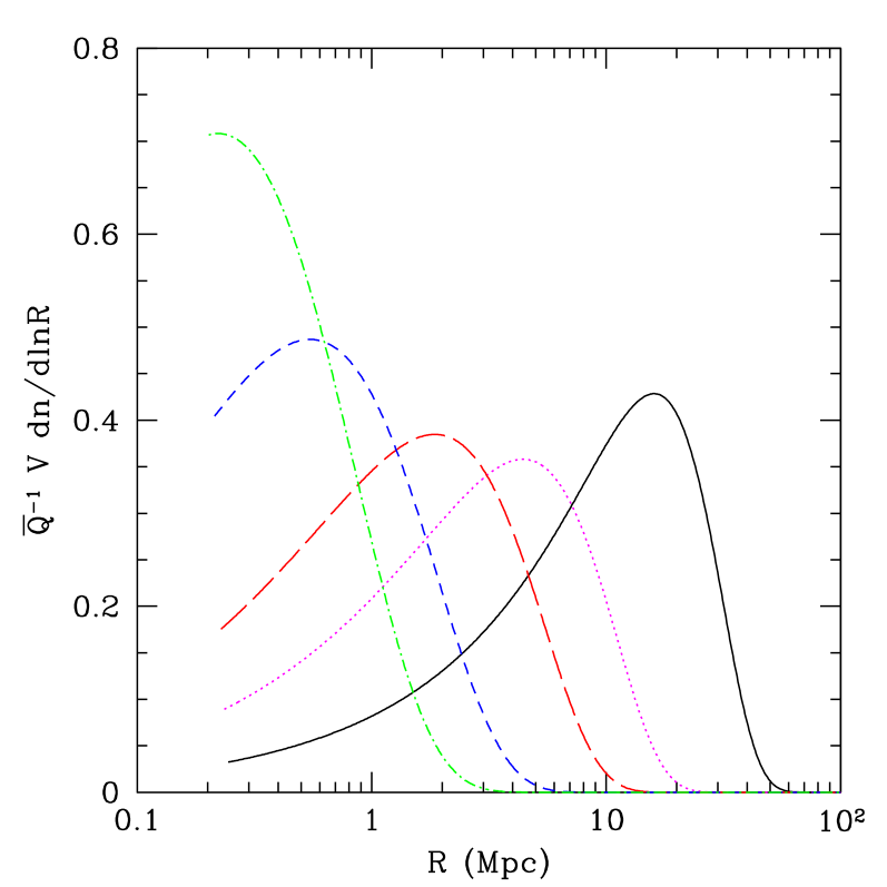
Figure 1: The bubble size distribution $\bar{Q}^{-1}Vdn/d\ln R$ at several different redshifts in our model, assuming $\zeta=40$ (note that $R$ is the comoving size). Dot-dashed, short-dashed, long-dashed, dotted, and solid lines are for $z=18,\,16,\,14,\,13$, and $12$, respectively. These have $\bar{Q}=0.037,0.11,0.3,0.5$, and $0.74$.

We refer the reader to FZH04 for a more in-depth discussion of this formalism.

3 Ly$\alpha$ Emitters

We will first consider the how the topology of HII regions affects galaxies with strong Ly$\alpha$ emission lines. The essential idea is that absorption from the surrounding neutral gas will modify the observed line; in the simplest approximation, Ly$\alpha$ lines will be much harder to see as $\bar{x}_{H}$ increases because of the increased absorption. In §3.1 we calculate the probability for a galaxy of a given mass to sit inside an ionized bubble of a given size. We will then describe in §3.2 how the resulting distribution affects the prospects for surveys of Ly$\alpha$ emitters.

3.1 Galaxies and Their HII Regions

We wish to know the probability $p(m_{b}|m_{h})$ that a halo of mass $m_{h}$ sits inside of an HII region with mass $m_{b}$ (corresponding to a radius $R_{b}$). One of the advantages of using the excursion set formalism to model both the HII regions and the dark matter halos is that it is straightforward to connect the two objects; the argument is similar to the treatment of non-gaussianity in §5 of FZH04 and to the derivation of the conditional halo mass function (Lacey & Cole, 1993). We wish to compute the probability that a trajectory crossing the halo mass function barrier $\delta_{c}$ at $\sigma^{2}_{h}$ has previously crossed the ionization barrier $\delta_{x}$ (or $B$ in our approximation) at $\sigma^{2}_{b}>\sigma^{2}_{h}$. (We will use the subscript “b” to refer to an ionized bubble and “h” to refer to the galaxy halo.) The distribution of first-crossings above $\delta_{c}$, $p(\delta^{f}_{h}=\delta_{c})$ (here the “f” superscript indicates a first-crossing) corresponds to the halo mass function (Press & Schechter, 1974; Bond et al., 1991). Similarly, the distribution of first-crossings above $B$, $p(\delta^{f}_{b}=B)$, can be found directly from equation (2). Moreover, given that a particle trajectory crosses $B$ at $\sigma^{2}_{b}$ (i.e., that this particle is part of an HII region of mass $m_{b}$), we can construct the conditional halo mass function in the usual way by translating the origin to $[\sigma^{2}_{b},\delta=B(m_{b})]$ (Lacey & Cole, 1993). We call this conditional probability $p(\delta^{f}_{h}=\delta_{c}|\delta^{f}_{b}=B)$. Then we use Bayes’ theorem to find $p(\delta^{f}_{b}=B|\delta^{f}_{h}=\delta_{c})$, the probability that a trajectory is part of an HII region of mass $m_{b}$ given that it is part of a collapsed halo with mass $m_{h}$:

$$p(\delta^{f}_{b}=B|\delta^{f}_{h}=\delta_{c})p(\delta^{f}_{h}=\delta_{c})d\delta_{b}\ =$$

$$\qquad p(\delta^{f}_{h}=\delta_{c}|\delta^{f}_{b}=B)p(\delta^{f}_{b}=B)d\delta_{b}.$$ (3)

The last three terms are all known, so the conditional probability is straightforward to compute. We can obtain the desired result by simply transforming to mass units:

$$p(m_{b}|m_{h})dm_{b} = \sqrt{\frac{2}{\pi}}\ \frac{B_{0}[\delta_{c}-B(m_{b})]}{\delta_{c}}\ \left|\frac{d\ln\sigma_{b}}{d\ln m_{b}}\right|$$ (4)

$$\times\exp\left\{-\frac{[\sigma_{b}^{2}\delta_{c}-\sigma_{h}^{2}B(m_{b})]^{2}}{2\sigma_{b}^{2}\sigma_{h}^{2}(\sigma_{h}^{2}-\sigma_{b}^{2})}\right\}$$

$$\times\frac{\sigma_{h}^{3}}{\sigma_{b}(\sigma_{h}^{2}-\sigma_{b}^{2})^{3/2}}\frac{dm_{b}}{m_{b}},$$

where $B_{0}$ is defined above equation (2) and is found from $B_{0}\equiv\delta_{x}(m=\infty)$. An implicit assumption behind equation (4) is that the density distribution $p(\delta)$ on the relevant mass scales is gaussian. This approximation breaks down on sufficiently small scales, and we expect that early in reionization (when the HII regions are small) our formalism will be less accurate. (Note that in this regime our linear approximation for $\delta_{x}$ is also only approximate.)

We show the cumulative probabilities that galaxies of mass $m_{h}=10^{9}\mbox{ M${}_{\odot}$}$ and $m_{h}=10^{11}\mbox{ M${}_{\odot}$}$ are in bubbles with radius above some value in Figure 2 for the choice $\zeta=40$. (This choice leads to reionization at $z\sim 11$.) Each curve begins at the minimum bubble size to contain such an ionizing galaxy, $\zeta m_{h}$ (i.e., the radius of the Strömgren sphere if the galaxy had no neighbors). We see that including neighboring galaxies makes a dramatic difference to the host HII regions of these galaxies. In both cases, nearly half are in regions at least twice the radius of the naive estimate by the time $\bar{x}_{H}\sim 0.5$, and there is a significant tail extending to much larger bubbles even earlier. This is a good illustration of one of the principal conclusions of FZH04: the distribution of bubble sizes is determined not by the characteristics of individual galaxies but instead by the large-scale density field. The tail at large $R_{b}$ is more significant for smaller galaxies, because the most massive halos are less likely to have neighbors of comparable or greater mass so contribute relatively more to the local ionizing field. Also, note that the distribution clearly evolves rapidly throughout reionization, with the fastest evolution occurring in the regime $\bar{x}_{H}\la 0.5$.

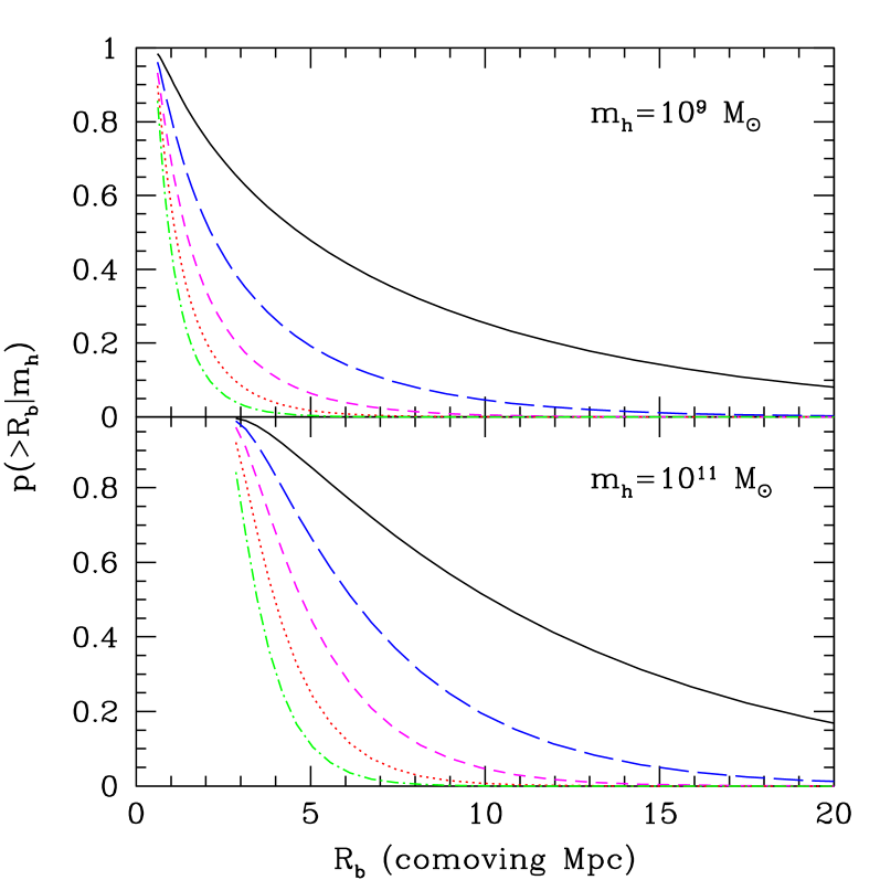
Figure 2: The probability that halos with $m_{h}=10^{9}$ and $10^{11}\mbox{ M${}_{\odot}$}$ are embedded in an HII region above a given comoving radius in the $\zeta=40$ model (top and bottom panels, respectively). The curves correspond to: $z=12$ ($\bar{x}_{H}=0.26$, solid), $z=13$ ($\bar{x}_{H}=0.52$, long-dashed), $z=14$ ($\bar{x}_{H}=0.7$, short-dashed), $z=15$ ($\bar{x}_{H}=0.81$, dotted), and $z=16$ ($\bar{x}_{H}=0.89$, dot-dashed).

Figure 2 reveals a minor inconsistency of our approach: the total probability for a galaxy to be in an HII region with $m_{b}>\zeta m_{h}$ is not equal to unity, as required by our fundamental assumption (see §2). Unfortunately, there is nothing in the excursion set result (4) to guarantee this. For example, imagine a trajectory that maintains $\delta\sim 0$ until $m\sim m_{h}$ and then rises steeply to pass through $(\sigma^{2}_{h},\delta_{c})$. Such a trajectory is (by construction) part of a halo of mass $m_{h}$, but our formalism would assign it to an ionized bubble of mass $m_{b}\sim m_{h}$. Essentially this trajectory corresponds to an isolated halo that lacks any neighbors. Fortunately, these steep trajectories are rare, especially once the characteristic size of HII regions exceeds $\zeta m_{h}$ (which happens relatively early for most galaxy masses). We note that in the Lacey & Cole (1993) merger tree picture, these objects are halos that undergo no major mergers in the future, so they must be rare in a hierarchical structure formation scenario. The discrepancy is worst early in reionization, when $\delta_{x}$ is large and therefore more difficult to cross. Figure 2 shows that, even when $\bar{x}_{H}\sim 0.9$, only $\sim 15\%$ of halos are assigned to ionized bubbles whose nominal sizes are smaller than $\zeta m_{h}$. As expected, the fraction of these trajectories decreases rapidly and they can essentially be ignored once $\bar{x}_{H}\la 0.7$. The discrepancy is also slightly smaller for massive galaxies because $\delta_{c}-\delta_{x}$ is an increasing function of mass (i.e., a trajectory must rise more steeply in order to be assigned to a small HII region). Physically, this is because more massive galaxies are also more highly biased.

We have shown $p(>R_{b}|m_{h})$ for only two masses in one particular model of reionization. Although the bubble size distribution at a fixed $\bar{x}_{H}$ is nearly independent of $\zeta$, the properties of the ionizing galaxies clearly do change between different reionization scenarios. Most importantly, the characteristic mass scale of the ionizing galaxies decreases if reionization occurs earlier. Qualitatively, the distributions shown in Figure 2 would correspond to smaller galaxies if $\zeta>40$ and larger galaxies if $\zeta<40$. Note that the two masses we have selected are both relatively rare at $z\sim 12$–$16$; galaxies closer to the nonlinear mass scale would experience even larger relative effects from the HII regions of their neighbors.

3.2 Observable Consequences

In principle, one way to constrain the ionization state of the IGM is to measure the amount of absorption from neutral gas outside of a galaxy’s HII region. The Hubble flow velocity offset between the galaxy and neutral gas implies that the Ly$\alpha$ photons redshift out of resonance by the time they encounter neutral gas. The relevant cross-section is therefore the “damping wing” of the line profile. Assuming that the galaxy is at $z_{\rm gal}$, with neutral gas between $z_{0}$ and $z_{n}$, the optical depth $\tau_{\rm damp}$ at $\lambda_{\rm obs}=\lambda_{\alpha}(1+z_{\rm gal})$ is (Miralda-Escude, 1998)

$$\tau_{\rm damp} = 6.43\times 10^{-9}x_{H}\tau_{\rm GP}(z_{\rm gal})$$ (5)

$$\times\ \left[I\left(\frac{1+z_{n}}{1+z_{\rm gal}}\right)-I\left(\frac{1+z_{0}}{1+z_{\rm gal}}\right)\right],$$

where $\lambda_{\alpha}=1215.67$ Å, $\tau_{\rm GP}(z_{\rm gal})\sim 6.5\times 10^{5}[(1+z_{\rm gal})/10]^{3/2}$ is the Ly$\alpha$ optical depth for a fully neutral IGM (Gunn & Peterson, 1965), $x_{H}$ is the neutral fraction outside of the HII region, and

$$I(x) = \frac{x^{9/2}}{1-x}+\frac{9}{7}x^{7/2}+\frac{9}{5}x^{5/2}+3x^{3/2}+9x^{1/2}$$ (6)

$$-\frac{9}{2}\ln\left(\frac{1+x^{1/2}}{1-x^{1/2}}\right).$$

Here we have assumed that $z_{0}<z_{n}<z_{\rm gal}$ and made the high redshift approximation $H(z)\propto(1+z)^{3/2}$.

The distribution of bubble sizes given in equation (4) can strongly affect the damping wing absorption of a galaxy’s Ly$\alpha$ line by pushing the neutral gas much farther from the galaxy than one would naively expect. By decreasing $z_{n}$, we increase the velocity separation between the emission line and the neutral gas, so that the galaxy line suffers less absorption. Neglecting peculiar velocities, the damping wing absorption depends only on the separation between the galaxy and the edge of the HII region. It is thus straightforward to transform equation (4) into the distribution of $\tau_{\rm damp}$. The only subtlety is that the galaxy need not sit exactly in the center of its ionized bubble. We will assume for simplicity that galaxies are uniformly distributed throughout the HII region, with the only restriction that each be a distance $R_{\rm min}$ from the edge. We set $R_{\rm min}$ equal to the radius of the galaxy’s HII region if it were completely isolated, because its own photons guarantee that the galaxy sits at least this distance from the nearest neutral gas. Note that the extreme assumption that all galaxies sit precisely in the center of the ionized bubble changes our results by $\la 25\%$ (much less in most cases). The true distribution will be somewhere in between these, because high-redshift galaxies are highly biased.

Figure 3 shows the resulting distributions for the same galaxies considered in Figure 2. In each case we scale $\tau_{\rm damp}$ to the value it would have if the galaxy were completely isolated, $\tau_{\rm iso}$; the corresponding values at $z=12$ are marked for the two halo masses. (Note that $\tau_{\rm damp}$ is $\sim 30\%$ higher at $z=16$; see equation [5].) To compute $\tau_{\rm damp}$, we have assumed that $\Delta z_{d}\equiv z_{n}-z_{0}=0.5$ and $x_{H}=1$ in this region. The true path length of neutral gas depends on the distance between individual HII regions and will evolve as the bubbles grow and overlap. We have ignored this effect for simplicity because it does not affect the main thrust of our argument. We consider a more detailed model in §4. Our choice here essentially maximises the damping wing absorption because gas beyond $\Delta z_{d}=0.5$ is far enough away in velocity space to render its absorption unimportant. The simplest refinement would be to scale $\tau_{\rm damp}$ by the mean neutral fraction, $\bar{x}_{H}$ (see §4.2). Note that we also neglect absorption by gas within the ionized bubble; we show below that this resonant absorption is subdominant at the line center (and especially on the red side) except when $\tau_{\rm damp}\la 1$.

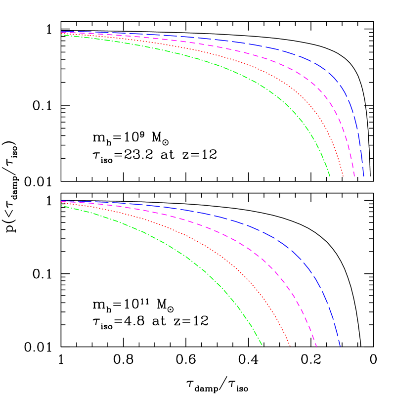
Figure 3: The probability that halos with $m_{h}=10^{9}\mbox{ M${}_{\odot}$}$ and $m_{h}=10^{11}\mbox{ M${}_{\odot}$}$ have a damping wing optical depth below some value in the $\zeta=40$ model. In each case we parameterise $\tau_{\rm damp}$ in terms of the value it would have if only the galaxy’s own HII region surrounded it, $\tau_{\rm iso}$. The curves correspond to: $z=12$ ($\bar{x}_{H}=0.26$, solid), $z=13$ ($\bar{x}_{H}=0.52$, long-dashed), $z=14$ ($\bar{x}_{H}=0.7$, short-dashed), $z=15$ ($\bar{x}_{H}=0.81$, dotted), and $z=16$ ($\bar{x}_{H}=0.89$, dot-dashed).

The figure shows that there is a non-negligible probability of substantially reduced absorption even early on, when $\bar{x}_{H}=0.9$: $\sim 20\%$ of $10^{9}\mbox{ M${}_{\odot}$}$ galaxies have $\tau_{\rm damp}<15$ and $\sim 5\%$ have $\tau_{\rm damp}<6$. As described above, the relative effects are larger for smaller galaxies, because they are more likely to have massive neighbors. Of course, the absolute $\tau_{\rm damp}$ is still significantly smaller for larger galaxies. If plotted as a function of $\tau_{\rm damp}$, we note that the probability distribution becomes less dependent on galaxy mass once the characteristic bubble size exceeds $R_{\rm min}$.

As emphasised above, the damping wing absorption depends on the IGM characteristics. If the IGM is partially ionized, either from an earlier episode of reionization or from a smooth ionizing component such as X-rays (e.g., Oh 2001; Venkatesan et al. 2001), $\tau_{\rm damp}$ decreases for two reasons. Obviously, the intrinsic damping wing is weaker if the external IGM is partially ionized. This effect could be accounted for by simply rescaling $\tau_{\rm iso}$ in Figure 3. However, the HII regions will also be larger for a given ionizing luminosity, because fewer photons are consumed in ionizing each IGM volume element. As another example, we can consider “double reionization” scenarios. An early generation of sources can imprint a characteristic bubble size on the IGM that persists until the second generation of sources has produced more ionizing photons than the first generation (Furlanetto et al., 2004a). In this case the damping wing absorption would be determined by the relic bubbles from the first generation. Thus the distribution of $\tau_{\rm damp}$ can constrain complex reionization histories as well as the relatively simple ones we have explicitly considered.

In principle, the damping wing absorption experienced by a galaxy inside an HII region could be modified by its peculiar velocity. However, this turns out to be unimportant: the typical velocity of a halo at $z\sim 10$ is $\sim 100\mbox{ km s${}^{-1}$}$ (Sheth & Diaferio, 2001), much smaller than the Hubble flow difference across its own Strömgren sphere. Actually, the relative velocity shift between the galaxy and the edge of the HII region is significantly smaller, because linear theory peculiar velocities are determined by the mass distribution on the largest scales and have fairly gentle gradients on Mpc scales. Peculiar velocities could be more important for resonant absorption, but nonlinear effects, including gas infall and internal motions such as winds, are likely much more significant (Santos, 2004).

We see that the distribution of damping wing absorption is broad and, especially during the middle and late stages of reionization, does not directly map onto the ionizing output of an embedded galaxy. Thus it appears dangerous to attempt to constrain the ionization state of the IGM outside of the Strömgren sphere by comparing the inferred absorption of the line to the estimated ionizing luminosity (even neglecting the many complications intrinsic to the galaxy; Santos 2004). Instead, the galaxy’s neighbors play a crucial role in determining the topology of ionized gas. Thus we suggest that attempts to infer the reionization history through observations of individual high-redshift galaxies (e.g., Rhoads & Malhotra 2001; Loeb et al. 2004; Cen et al. 2004) are highly uncertain. For example, Hu et al. (2002) and Rhoads et al. (2004) claim that observations of strong Ly$\alpha$ emission lines at $z\sim 6.5$ require the galaxies to be embedded in a mostly ionized medium. Our model predicts that a galaxy with $m_{h}=10^{10}\mbox{ M${}_{\odot}$}$ has a $(0.3\%,16\%,55\%)$ chance of $\tau_{\rm damp}<2$ if $\bar{x}_{H}=(0.75,0.5,0.25)$ at $z=6.5$. These become $(1\%,33\%,73\%)$ if $m_{h}=10^{11}\mbox{ M${}_{\odot}$}$. Thus, it seems likely that $\bar{x}_{H}\la 0.5$, but stronger conclusions are currently unwarranted.

On the other hand, our results suggest that searches for high-redshift Ly$\alpha$ emitters can easily be extended to the era before reionization. While some fraction of galaxies will have their Ly$\alpha$ lines completely absorbed by the surrounding IGM, many will retain strong lines that can be isolated in narrow-band searches. Most interestingly, the distribution of inferred damping wing optical depths yields a measurement of the sizes of HII regions, which in turn tells us about the morphology of reionization. Of course, we must account for effects intrinsic to the galaxy and its immediate environments before strong constraints will emerge.

One potential difficulty with surveys beyond reionization is that cosmic variance could become extremely large, because the local overdensity of galaxies modulates the damping wing absorption. We illustrate this point in Figure 4. We first make the simplest possible assumption that the Ly$\alpha$ line luminosity is proportional to the galaxy mass, and we suppose that a given survey can probe down to a minimum mass $m_{\rm obs}$, neglecting any IGM absorption. This is obviously a poor assumption, because galaxies of a single mass can have a wide range of star formation rates, wind velocities, and intrinsic absorption, but it is probably not too bad in the statistical sense. We wish to find the fraction of galaxies with mass $m_{h}$ that would be observable by such a survey and how they are distributed in space. Our assumptions require that a galaxy have damping wing absorption $\tau_{\rm damp}$ smaller than $\tau_{\rm max}\equiv\ln(m_{h}/m_{\rm obs})$ in order to be in the survey.

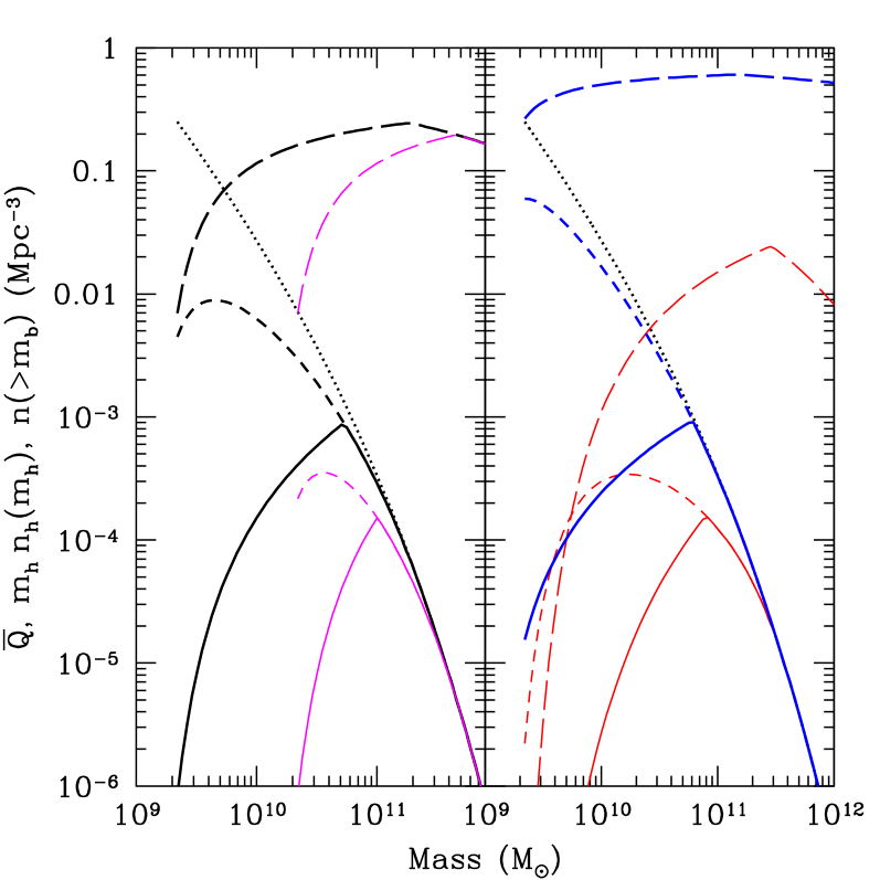
Figure 4: Cosmic variance in Ly$\alpha$ selected surveys at $z=8$. The dotted curves show the (logarithmic) halo mass function, $m_{h}n_{h}(m_{h})$. Short-dashed curves show the number density of halos that are visible given a minimum observable galaxy mass, $m_{\rm obs}$. Solid curves show the approximate number density of HII regions of which these observable galaxies can be part, $n(>m_{b})$, while the long-dashed curves show the fraction of space filled by these bubbles ($\bar{Q}$). The left panel assumes $\bar{x}_{H}=0.5$, with $m_{\rm obs}=10^{9}$ and $10^{10}\mbox{ M${}_{\odot}$}$ for the thick and thin curves, respectively. The right panel assumes $m_{\rm obs}=10^{9}\mbox{ M${}_{\odot}$}$, with $\bar{x}_{H}=0.75$ and $0.25$ for the thick and thin curves.

The dotted curves in Figure 4 show the halo mass function (Press & Schechter, 1974). The short-dashed curves show the fraction of galaxies at each mass that are accessible to our example survey, using the formalism described above. The solid curves show the number density of HII regions that have $\tau_{\rm damp}<\tau_{\rm max}$ at their central points, while the long-dashed curves show the fraction of space filled by such regions, $\bar{Q}$. The left panel shows results for two different mass thresholds, $m_{\rm obs}=10^{9}$ and $10^{10}\mbox{ M${}_{\odot}$}$ (thick and thin curves, respectively) if $\bar{x}_{H}=0.5$ at $z=8$. The number of visible sources is small near the mass threshold, because the sources must be embedded in extremely large bubbles, and they are confined to rare regions of the universe (though the total number density is not small). As $m_{h}$ increases, however, the fraction of visible galaxies rapidly approaches unity and the fraction of the universe through which they are distributed also increases. (Note that $\bar{Q}$ decreases for sufficiently massive galaxies because these galaxies are themselves so rare.) This is because the intrinsic luminosity is so large that they are visible even when completely isolated. The right panel shows results for $m_{\rm obs}=10^{9}\mbox{ M${}_{\odot}$}$ if $\bar{x}_{H}=0.75$ and 0.25 (thick and thin curves, respectively). Note the dramatic decline in the volume available to the survey when $\bar{x}_{H}=0.25$; while some fraction of galaxies are still visible, they are widely separated and highly clustered. Large-volume surveys will therefore be required, especially in the earlier stages of reionization.

Finally, to further illustrate the importance of the size distribution of bubbles, we now calculate some example emission line profiles. We will take as an illustrative example a galaxy with $m_{h}=10^{9}\mbox{ M${}_{\odot}$}$ at $z=10$. Given a bubble size, we compute the damping wing absorption from equation (5). However, in this case we must also include the absorption by the (mostly ionized) gas near the galaxy. This gas is in ionization equilibrium, so (neglecting clumping)

$$\alpha_{B}n_{H}^{2}(z)=x_{H}n_{H}(z)\bar{\sigma}(1+z)^{2}\frac{\dot{N}_{\gamma}}{4\pi R^{2}},$$ (7)

where $\alpha_{B}$ is the case B recombination coefficient, $\bar{\sigma}\approx 2\times 10^{-18}\mbox{ cm${}^{2}$}$ is the frequency-averaged ionization cross-section, $R$ is the distance in comoving units, and $\dot{N}_{\gamma}$ is the rate at which the central source produces ionizing photons. To compute this quantity, we include only the ionizing photons from the galaxy (which dominate the background at the relevant distances). We assume a star formation rate of $3\mbox{ M${}_{\odot}$ yr${}^{-1}$}$, with the ionizing photon production rate given by Leitherer et al. (1999) for continuous star formation at $Z=0.05Z_{\odot}$ and with a Salpeter initial mass function and a low-mass cutoff of $M=1\mbox{ M${}_{\odot}$}$. We then allow a fraction $f_{\rm esc}=0.05$ of these to escape the galaxy. These parameters are of course arbitrary, but they could describe the putative $z=10$ galaxy discovered by Pelló et al. (2004). For reference, these nominal parameters would correspond to $\zeta=400f_{\star}/(1+n_{\rm rec})$, where $f_{\star}$ is the nominal star formation efficiency and $n_{\rm rec}$ is the mean number of times a hydrogen atom recombines. Finally, we assume that the line width is $\sigma_{v}=V_{c}/\sqrt{2}$, where $V_{c}$ is the circular velocity of the halo (Barkana & Loeb, 2001); this yields $\sigma_{v}=27\mbox{ km s${}^{-1}$}$ for our parameters..

Equation (7) yields the profile of $x_{H}$ near to the galaxy. To compute the resonant optical depth $\tau_{\rm res}$ at a particular observed wavelength $\lambda_{\rm obs}$, we integrate the Ly$\alpha$ absorption cross-section over this $x_{H}$ distribution, assuming pure Hubble flow for the velocity structure. We assume a Voigt profile with $T=10^{4}\mbox{ K}$ for the absorption cross section, as appropriate for ionized gas. We note here that our treatment of resonant absorption is highly simplified and neglects many important effects. For example, we have assumed the gas to be smoothly distributed at the mean density; in reality it will have a complicated density distribution. Lines of sight passing through overdense regions will have correspondingly more absorption; however, most of space is filled by underdense gas and the mean resonant absorption is somewhat weaker. We estimate this effect in §4.3 below. We have also neglected infall and winds, which move the gas through velocity space and can in principle strongly affect the absorption (Santos, 2004). Fortunately, neither of these effects change our qualitative result, so we will not discuss them further here.

Several example line profiles are shown in Figure 5, along with the corresponding optical depths. The solid, long-dashed, short-dashed, and dot-dashed lines assume $R_{b}=10,\,5,\,3$, and $1\mbox{ Mpc}$, respectively. (The last of these is nearly completely absorbed by the damping wing and does not appear in the top panel.) In the top panel, the upper dotted curve shows the assumed intrinsic line profile; the other dotted line shows the absorption profile for $R_{b}=10\mbox{ Mpc}$ if we neglect resonant absorption. In the bottom panel, the dotted line shows $\tau_{\rm res}$. For reference, an isolated galaxy of this mass should have $R_{b}^{\rm iso}\approx(\zeta/160)^{1/3}\mbox{ Mpc}$. As a fiducial example, $\zeta=12$ implies $\bar{x}_{H}=0.5$ at this redshift. Then a galaxy with $m_{h}=10^{9}\mbox{ M${}_{\odot}$}$ would have a $(75\%,\,40\%,\,20\%,\,3\%)$ probability of being in bubbles larger than $(1,\,3,\,5,\,10)\mbox{ Mpc}$ according to our formalism. It is obvious that the large-scale environment of the galaxy dramatically affects its absorption properties. While the resonant absorption will suppress the blue side of the line, it has little effect on the red side, which allows an estimate of $\tau_{\rm damp}$.

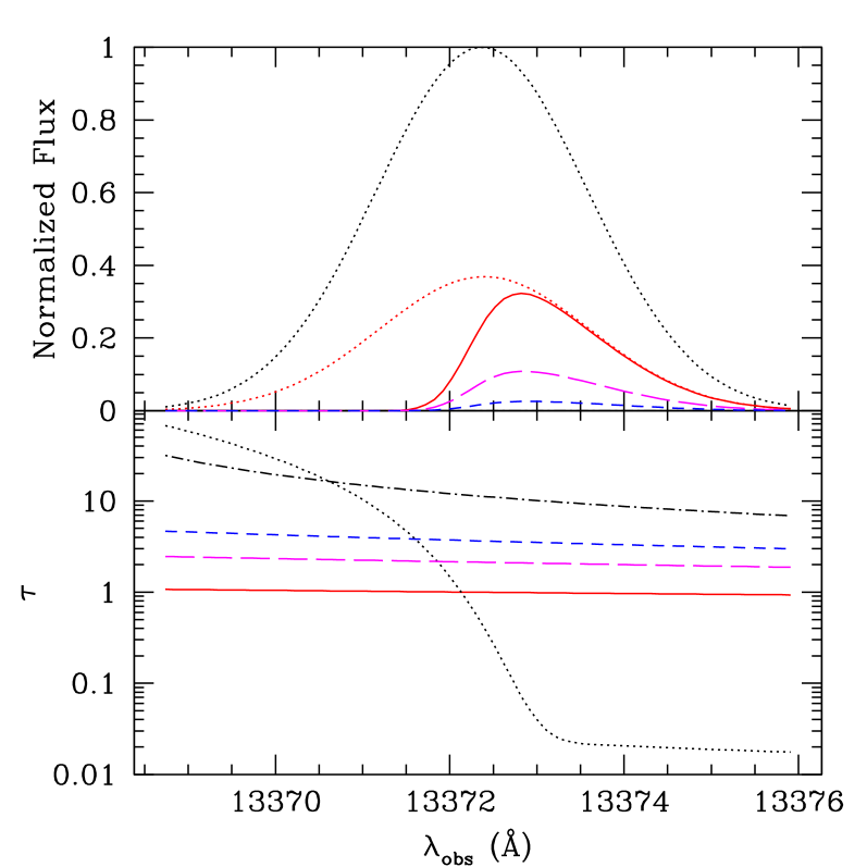
Figure 5: Top panel: Example line profiles for a galaxy at $z=10$. The upper dotted curve shows the assumed intrinsic profile. The solid, long-dashed, and short-dashed curves place the galaxy in HII regions of comoving size $R_{b}=10,\,5$, and $3\mbox{ Mpc}$, respectively. The lower dotted curve shows the absorption profile for $R_{b}=10\mbox{ Mpc}$ if we neglect resonant absorption. Bottom panel: The solid, long-dashed, short-dashed, and dot-dashed curves show $\tau_{\rm damp}$ if the galaxy is in an HII region of comoving size $R_{b}=10,\,5,\,3$, and $1\mbox{ Mpc}$, respectively. The dotted line shows $\tau_{\rm res}$, which is the same for all bubble sizes.

4 Transmission Gaps in the Gunn-Peterson Trough

We now consider whether HII regions can appear as gaps in the Gunn-Peterson troughs of distant quasars (unrelated to the ionized bubbles that we wish to observe). We will compute

$$\frac{dn(<\tau)}{dz}=\frac{dr}{dz}\int dm\,n(m)\pi R^{2}_{\rm max}(m,\tau),$$ (8)

where all distances are in comoving units, $dn(<\tau)/dz$ is the number of transmission gaps with optical depths smaller than $\tau$ per unit redshift, and $n(m)$ is the mass function of ionized regions. $R_{\rm max}$ is the impact parameter from the center of the HII region at which the optical depth is $\tau$. Note that the total optical depth is twice the damping absorption (because both the blue and red sides contribute) plus the resonant absorption. We compute the minimum optical depth encountered within each HII region (i.e., when the line of sight passes closest to the center of the bubble).

We first estimate the resonant absorption inside the ionized bubbles in §4.1. We then present the resulting absorption statistics in §4.2 and estimate how the inhomogeneous IGM affects our results in §4.3. Finally, we discuss the spectrum of SDSS J1148+5251 in §4.4.

4.1 Resonant Absorption

Figure 5 shows that resonant absorption is relatively unimportant for Ly$\alpha$ emitters (at least on the red side of the line). This is because photons emitted on the red side never pass through the Ly$\alpha$ resonance in the IGM and because the object we are observing creates a local, highly-ionized bubble around itself. The resonant absorption within this zone is suppressed because $x_{H}$ is much lower near the galaxy. However, for lines of sight on a random path through an HII region, the probability of passing so close to an ionizing source is small. Thus most will suffer substantial resonant absorption.

To compute $\tau_{\rm res}$, we therefore need to know the distribution of ionizing sources within the HII region. We will begin by examining two simple limiting cases. In the end, we will show that they yield nearly identical results. First, let us assume that all of the ionizing sources are located in the center of the bubble. In that case, we can use equation (7) once we have an estimate for $\dot{N}_{\gamma}$. Unfortunately, this factor does not follow directly from the formalism described in §2. Our model uses the total time-integrated number of ionizing photons (essentially our $\zeta$ parameter) to compute the bubble sizes, while we need the instantaneous photoionization rate to compute $x_{H}(R)$. For simplicity, we will assume that each HII region contains many sources, so that their fluctuating star formation rates average out. This is obviously only accurate in the late stages of reionization, when the bubble sizes are much larger than those of individual galaxies; fortunately, this regime will turn out to be the relevant one anyway. In this case, we can set

$$\dot{N}_{\gamma}=\frac{\zeta m_{b}}{\mu m_{H}}\dot{f}_{\rm coll}$$ (9)

for a bubble of mass $m_{b}$. Then

$$x_{H}^{c}(R) = \frac{3\alpha_{B}}{\bar{\sigma}R_{b}H(z)}\ \left(\frac{R}{R_{b}}\right)^{2}\ \left(\frac{f_{\rm coll}}{|df_{\rm coll}/dz|}\right)$$

$$\approx 3.2\times 10^{-3}\,\left(\frac{{\rm Mpc}}{R_{b}}\right)\ \left(\frac{R}{R_{b}}\right)^{2}\ \left(\frac{10}{1+z}\right)^{2}$$

$$\times\ \left(\frac{f_{\rm coll}}{|df_{\rm coll}/dz|}\right)\ \left(\frac{0.15}{\Omega_{m}h^{2}}\right)^{1/2},$$

where the “c” superscript refers to the case in which all the ionizing sources are at the center of the bubble. Note that the $f_{\rm coll}$ factor is typically of order 3 at these redshifts. The resonant absorption at the specified velocity is then $\tau_{\rm res}\approx\tau_{\rm GP}x_{H}$ and will be quite large except near the center of the regions. We have ignored one subtlety in equation (9): in general $\zeta$ includes the mean number of recombinations $n_{\rm rec}$ in the IGM, integrated over the entire reionization history to this point. The instantaneous ionizing rate, of course, does not depend on the recombination rate in the past. Thus $x_{H}^{c}\propto(1+n_{\rm rec})^{-1}$; in a scenario in which recombinations have delayed reionization but the mean ionizing emissivity is high, this could have a substantial effect.

As a second limiting case, we assume that the sources are distributed uniformly throughout the bubble. In this case the flux of ionizing photons is also approximately uniform across the HII region (non-uniformity occurs only because the bubble has a finite size); in equation (7), we have

$$\frac{\dot{N}_{\gamma}}{4\pi R^{2}}\rightarrow\frac{3\dot{N}_{\gamma}}{4\pi R_{b}^{2}}.$$ (11)

The resulting ionized fraction is

$$x_{H}^{u}=x_{H}^{c}(R_{b})/3.$$ (12)

We find that the resonant absorption is $\tau_{\rm res}\sim 10^{-3}\tau_{\rm GP}(z)({\rm Mpc}/R_{b})$ at a typical position within a bubble, or $\tau_{\rm res}\ga 60$ for $R_{b}=10\mbox{ Mpc}$. Thus the mean neutral fraction is large, so $\tau_{\rm res}\gg 1$ unless the line of sight passes close to an ionizing source. This has a fortunate consequence: the cross-section for a line of sight with $\tau_{\rm res}<\tau_{0}$ is independent of the number of sources (see also Barkana 2002). Suppose that the bubble is made up of $N$ identical galaxies. From equation (7), the radius at which the optical depth equals a fixed value $\tau_{0}$ is $R_{\rm max}(\tau_{0})\propto 1/\sqrt{N}$. Thus the total cross-section through such regions is $N\times\pi R_{\rm max}^{2}=$ constant and is independent of the number of “subclusters” within the HII region. A similar argument shows that the cross-section also remains unchanged if only a fraction of the bubbles are “active” at a given time. Of course, if the galaxies or subclusters are distributed throughout the bubble, their damping wing absorption will change with distance from the edge. Because this is a relatively small effect, we will use equation (4.1) to compute the resonant absorption inside the HII regions.

Note that the above treatment assumes a uniform density IGM. We will show that clumping actually increases $R_{\rm max}$ in §4.3.

Both of the above prescriptions neglect absorption of the ionizing photons as they travel through the bubble. This requires the total optical depth to ionizing photons $\tau_{\rm ion}$ to be $\la 1$. We find that

$$\tau_{\rm ion}(R_{b}) = \frac{n_{H}(z)\alpha_{B}}{(1+z)H(z)}\ \left(\frac{f_{\rm coll}}{|df_{\rm coll}/dz|}\right)$$

$$\approx 0.1\left(\frac{f_{\rm coll}}{|df_{\rm coll}/dz|}\right)\ \left(\frac{1+z}{10}\right)^{1/2}$$

$$\times\ \left(\frac{0.15}{\Omega_{m}h^{2}}\right)^{1/2}\left(\frac{\Omega_{b}h^{2}}{0.023}\right),$$

in both the centrally concentrated and uniform limits. Thus, neglecting any dense clumps, the majority of ionizing photons reach the edge of the bubble without being consumed by recombinations. This is, in fact, a necessary assumption of the model described in §2. Of course, if a large fraction of lines of sight pass through dense “Lyman-limit” systems before hitting the edge of the bubble (or in other words if the characteristic bubble size exceeds the mean free path between such systems), the HII region would no longer expand and our model breaks down. The point at which this occurs is of course unknown; note that it could be quite early if “minihalos” are common (Barkana & Loeb, 2002).

4.2 The Abundance of Transmission Gaps

We are now in a position to compute $dn(<\tau)/dz$ from equation (8). We calculate the resonant absorption via the centrally concentrated limit of equation (4.1) and $\tau_{\rm res}\approx x_{H}\tau_{\rm GP}$. For the damping wing, we must know the total path length of the neutral segment of gas (i.e., $z_{n}-z_{0}$ in equation [5]). This is difficult to compute precisely, because it depends on the large-scale distribution of the HII regions. We will take $\Delta z_{d}=0.5$ and assume that the neutral fraction is $\bar{x}_{H}$ within this region. We examine the importance of this prescription below (where we also show some examples of $R_{\rm max}$).

Figure 6 shows how the absorption statistics evolve through reionization in our model. The thick and thin curves assume $\zeta=12$ and $40$, respectively. The differences between the two are relatively modest, despite being displaced in redshift by $\Delta z\sim 3$, and occur because the higher cosmic densities in the $\zeta=40$ model make absorption somewhat stronger. The curves are fairly flat until some characteristic optical depth is reached; this is because the bubbles themselves have a characteristic size. The curves flatten with time because resonant absorption becomes less significant as the bubbles grow and because the peak in the bubble size distribution sharpens with time. The expected number of absorbers is clearly quite small; even when $\bar{x}_{H}\sim 0.1$, only $\sim 0.1$ gaps with $\tau\la 4$ are expected per unit redshift. However, in contrast to Barkana (2002), the probability is not vanishingly small unless $\bar{x}_{H}\ga 0.5$. Even a few quasars shortly beyond reionization could show some transmission features. The difference arises because Barkana (2002) considered isolated HII regions around galaxies, for which the damping wing absorption provides a relatively large “floor” in the optical depth. In our model, the damping wing absorption can be much smaller at the centers of large bubbles. Finally, we have set $n_{\rm rec}=0$ when computing the resonant absorption (see the discussion of equation [4.1]). If recombinations have significantly delayed reionization, $dn/dz$ will increase approximately in proportion to $1/(1+n_{\rm rec})$, except at the bright end where the damping wing is important.

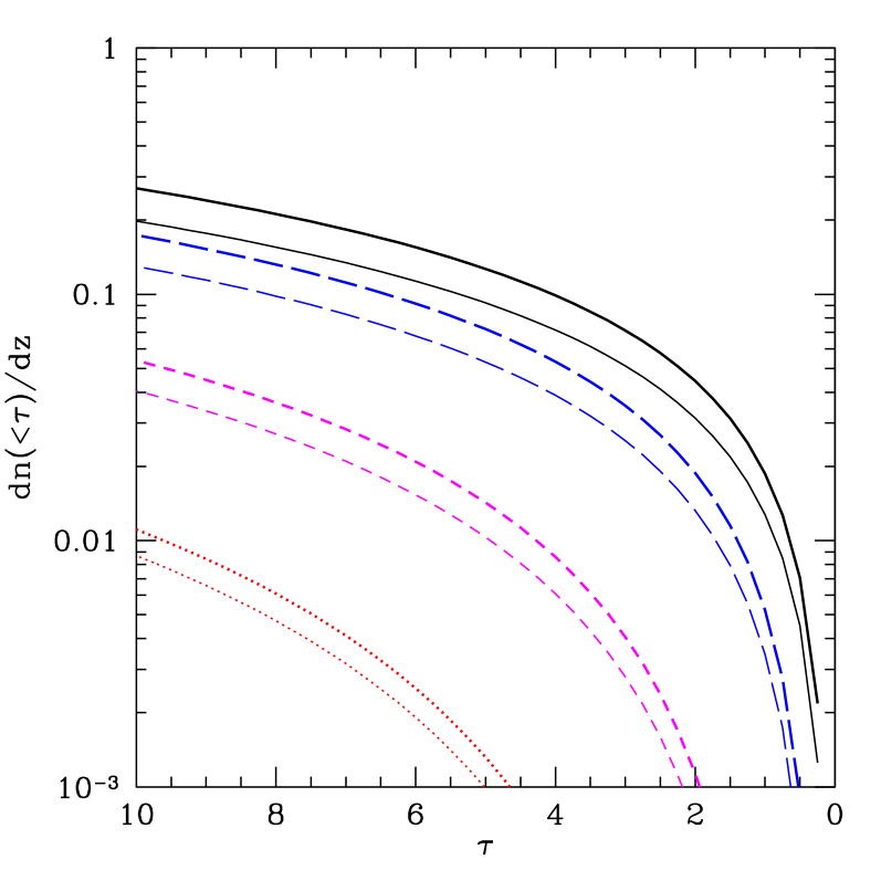
Figure 6: The number of transmission gaps per unit redshift $dn/dz$ with an optical depth smaller than the specified value. The thick curves assume $\zeta=12$ and have $\bar{x}_{H}=0.12$ ($z=8.5$, solid), $\bar{x}_{H}=0.3$ ($z=9$, long-dashed), and $\bar{x}_{H}=0.5$ ($z=10$, short-dashed), $\bar{x}_{H}=0.66$ ($z=11$, dotted). The thin curves assume $\zeta=40$ at the same neutral fractions; these occur $\Delta z\sim 3$ earlier than the thick curves.

We note here that it may be easier to detect regions of weak absorption in the Ly$\beta$ Gunn-Peterson trough, because $\tau_{\beta}=0.16\tau_{\alpha}$; the optical depth axis in Figure 6 can simply be scaled by this amount. We therefore expect a factor of several more such gaps near the end of reionization and orders of magnitude more during the early stages. Of course, the Ly$\beta$ region is blanketed by the lower-redshift Ly$\alpha$ forest, which will cover some fraction of the transmission gaps (especially since the Ly$\alpha$ forest should still be fairly deep at the relevant redshifts).

Assuming a uniform density IGM, we can easily estimate the widths of the transmission gaps. In the regime in which resonant absorption dominates, the optical depth will increase by a factor of two over a distance along the line of sight equal to the impact parameter: $\Delta\lambda/\lambda_{\rm obs}\sim H(z)R_{\rm max}/c\sim 0.003[(1+z)/10]^{3/2}(R_{\rm max}/{\rm Mpc})$. Interestingly, the line widths can thus break the degeneracy between a small number of clustered sources and a large number of distributed sources. As described above, the total cross section does not change if we separate the central ionizing source into $N$ small clusters, because $R_{\rm max}\propto N^{-1/2}$. However, each individual line of sight must pass closer to a source if clustering is weak, so the line widths would decrease. Similarly, if the central sources of HII regions are bursty, each “active” region would have a larger $R_{\rm max}$, making the individual lines larger. Note, however, that the optical depth gradients are much smaller if $\tau_{\rm damp}$ is important.

Figure 7 shows how our results depend on some of our input parameters. The top panel shows $R_{\rm max}$ if $\zeta=12$ and $z=9$ (at which time $\bar{x}_{H}=0.3$). The three solid curves correspond to $R_{b}=15,\,10$, and $5\mbox{ Mpc}$, respectively. In all cases, the impact parameter must be a small fraction of the total bubble size in order for the local ionizing background to be large enough to reduce the resonant absorption. The ratio $R_{\rm max}/R_{b}$ increases with $R_{b}$ both because the damping wing is farther away and because the source density increases. These curves change weakly with redshift because of the increased absorption in a denser universe. The other curves show how the results change with different assumptions about the damping wing. To construct the long-dashed curve, we assumed a fully neutral medium with $\Delta z_{d}=0.5$. The larger $\tau_{\rm damp}$ induces a more significant cutoff at the bright end, but the effects are not large at moderate optical depths because resonant absorption dominates. The short-dashed curve uses a prescription similar to that of Barkana (2002). We let $dn_{\rm ion}/dz$ be the number of ionized bubbles intersected per unit redshift; this is the same as equation (8) except that $R_{\rm max}\rightarrow R_{b}$. The mean path length of a neutral segment (in redshift units) is then given by $\bar{x}_{H}/\Delta z_{d}\sim{dn_{\rm ion}/dz}$. The damping wing absorption declines in this model because the path length between ionized bubbles is small. However, when $\bar{x}_{H}$ is small the prescription makes only a small difference because the damping wing is unimportant anyway.

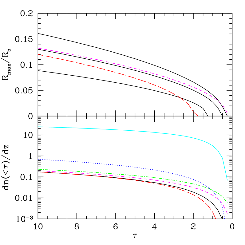
Figure 7: Top panel: The cross-section for bubbles. The solid curves have $R_{b}=15,\,10$, and $5\mbox{ Mpc}$, from top to bottom. The long and short dashed lines modify the damping wing (see text) and have $R_{b}=10\mbox{ Mpc}$. Bottom panel: Density of transmission gaps. The lower solid curve is our default model, and the long and short dashed lines modify the damping wing. The dotted line assumes that the resonant absorber has $\Delta=0.5$. The upper solid line includes only absorption from the damping wing, while the dot-dashed line includes only resonant absorption. All curves (in both panels) assume $\zeta=12$ and are at $\bar{x}_{H}=0.3$ ($z=9$).

The bottom panel of Figure 7 shows the effects on the transmission gap statistics. The lower solid curve is the normal model of Figure 6, while the dashed curves make the same assumptions as in the top panel. The effects on the gaps are clearly modest, except at the bright end. However, note that our assumptions about $\tau_{\rm damp}$ can be much more important for $\bar{x}_{H}\ga 0.5$, because even at that time $dn/dz_{\rm ion}$ can be relatively large (although the path length through each ionized bubble is small). Nevertheless, the number of observable transmission gaps is extremely small in this regime, even in the most optimistic scenario.

The upper solid curve is identical to our fiducial model except that we include only the damping wing component in the absorption. The amplitude is much larger in this case: as argued above, resonant absorption is the principal limiting factor in finding gaps. Comparing the small $\tau$ tails of the distributions, we see that the cutoff in the number of absorbers is fixed by the “floor” in damping wing absorption. In contrast, the dot-dashed curve includes only resonant absorption. The number density is not far from the full model (except at the bright end), indicating that this quantity controls the gap abundance. This has important implications for interpreting quasar spectra in light of complex reionization histories. Figure 6 assumes a simple model with a single generation of sources. The dominance of resonant absorption implies that the statistics will be qualitatively unchanged for more complex models, although we would expect a substantial increase in the number of nearly transparent gaps (with $\tau<1$). For example, if the external IGM is partially ionized, $\tau_{\rm damp}$ will decrease and the bubbles will be larger for a given ionizing emissivity. However, the resonant absorption within the bubbles will remain the same, and the dot-dashed curve shows an upper limit on the resulting number of gaps. Similarly, although an early generation of sources can increase the bubble size, it does not affect the resonant absorption. Thus we expect that $dn/dz$ places stronger constraints on the instantaneous ionizing emissivity than on the total ionized fraction, as long as the HII regions are large enough to reduce $\tau_{\rm damp}$ to a subdominant role. This could be especially interesting when combined with other methods (such as Ly$\alpha$ emitters or 21 cm tomography) that are more sensitive to the total ionization history.

4.3 The Effect of an Inhomogeneous IGM

The most important simplification we have made is to neglect the density distribution of the IGM. On the one hand, small-scale clumpiness increases the mean recombination rate and hence the resonant absorption inside bubbles. On the other hand, underdense regions with smaller optical depth fill most of the volume, so the majority of any line of sight is likely to pass through regions with smaller absorption. As a quick illustration, the long-dashed curve in Figure 7 shows how the results change if we assume that the gas causing resonant absorption has $\Delta=0.5$, where $\rho=\Delta\bar{\rho}$. Equation (7) shows that in ionization equilibrium the local neutral fraction is proportional to the local density, and the optical depth has an extra power of density. Thus $\tau_{\rm res}\propto\Delta^{2}$ at a fixed distance from the center of the bubble. This is close to the behavior we find in Figure 7 at moderate $\tau$, though the amplification is smaller at $\tau<1$ because the damping wing becomes important.

This is only the crudest estimate of the importance of density fluctuations. To do better, we must average the magnitude of absorption over the density structure of the IGM: we wish to compute $\tau_{\rm eff}\equiv-\ln\langle e^{-\tau}\rangle$ rather than simply $\langle\tau\rangle$ as we did above. The best way to approach the problem is with numerical simulations, but these are computationally expensive and cannot yet be performed with the necessary dynamic range. Here we take an approximate approach. We wish to estimate the fluctuations in the density field when smoothed along the line of sight over a thermal width of the absorbing gas. Miralda-Escudé et al. (2000) showed that the volume-averaged probability distribution of gas overdensity in numerical simulations at $z\sim 2$–$4$ is well fit by

$$P_{V}(\Delta)d\Delta=A\Delta^{-\beta}\exp\left[\frac{-(\Delta^{-2/3}-C)^{2}}{2(2\delta_{0}/3)^{2}}\right]d\Delta$$ (14)

when smoothed on the Jeans mass of the photoionized gas. The form is motivated by interpolating between linear theory and the growth of voids and halos in the nonlinear regime. The parameter $\delta_{0}$ describes the linear regime: Miralda-Escudé et al. (2000) find that it is given by $\delta_{0}=7.61/(1+z)$. The exponent $\beta$ depends on the density profile of collapsed objects; we will set $\beta=2.5$, the value it takes for isothermal spheres. We then fix the remaining parameters $A$ and $C$ by normalizing the mass and volume-weighted probability densities. Given the density distribution, we can compute the effective volume-averaged optical depth, $\tau_{\rm eff}$, corresponding to a nominal optical depth for the mean density IGM, $\tau_{\rm mean}$, through

$$\langle e^{-\tau}\rangle=\int d\Delta\,P_{V}(\Delta)\exp(-\tau_{\rm mean}\Delta^{2}).$$ (15)

Unfortunately, there are several reasons why this treatment is only approximate. First, Miralda-Escudé et al. (2000) used simulations with $\Omega_{m}=0.4$, $\Omega_{\Lambda}=0.6$, and $\sigma_{8}=0.79$, so there should be minor differences with the cosmology we have chosen. Moreover, the simulation did not resolve fluctuations on small scales: while the Jeans mass at $T=10^{4}\mbox{ K}$ is resolved, fluctuations on smaller scales are not. Such small scale clumpiness is probably not important at $z\sim 3$, for which the simulations were designed, because the thermal pressure of the ionized gas would have smoothed any density fluctuations. However, it may underestimate the fluctuations in recently ionized gas that has not yet relaxed into pressure equilibrium. Minihalos are an important example that could drastically increase the mean recombination rate until they photoevaporate (Barkana & Loeb, 2002; Shapiro et al., 2004). Furthermore, equation (14) smooths over the Jeans scale, which is slightly smaller than the thermal broadening width relevant for absorption studies. (However, we should also perform the average over one dimension rather than three.) Finally, equation (14) does not take into account the environment of the volume element under consideration. For resonant absorption, we are primarily concerned with regions that are near galaxies or groups of galaxies; we would therefore expect that the relevant regions would be less likely to contain a void. It is not clear which of these effects dominate, so we simply take equation (14) at face value and caution the reader that our results are only approximate.

We show the results of equation (14) in the top panel of Figure 8 for three different redshifts, $z=9,\,10$, and $11$ (from bottom to top). We see that $\tau_{\rm eff}$ decreases slowly as redshift decreases because structures condense and voids fill up more of the volume. The decrease in apparent optical depth is a factor of $\sim 3$–$4$ at moderate $\tau$. The difference becomes negligible for small $\tau$ (and close enough to zero, we even have $\tau_{\rm eff}>\tau_{\rm mean}$) as the extra clumpiness becomes important. The correction to $\tau$ is significantly smaller than that of Haiman (2002), who assumed a much clumpier density distribution.

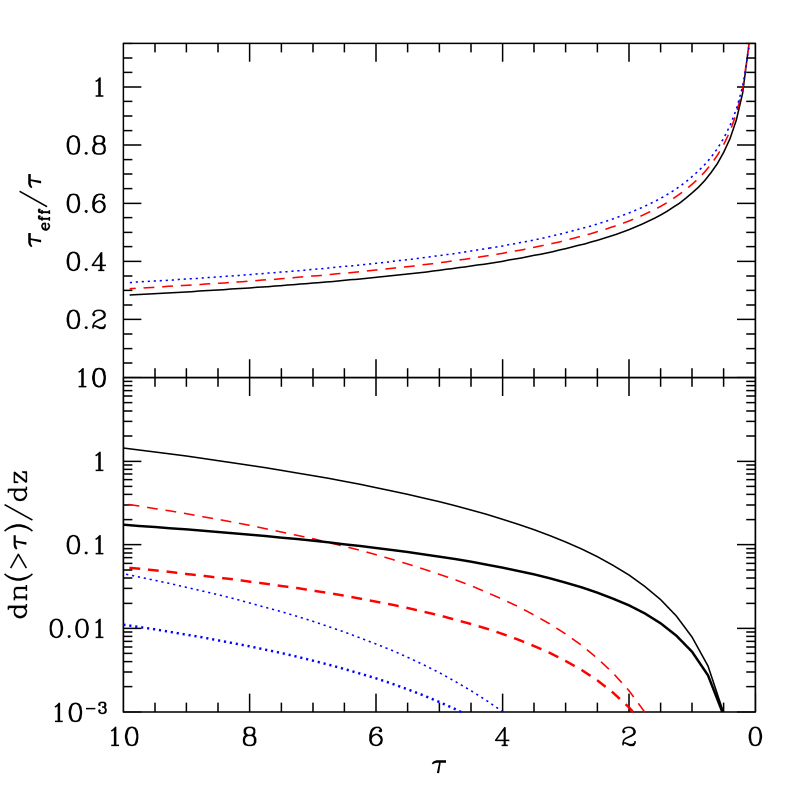
Figure 8: The top panel shows the ratio of $\tau_{\rm eff}=-\ln\langle e^{-\tau}\rangle$ to the optical depth of the mean density IGM, $\tau$, at $z=9,\,10$, and $11$ (solid, dashed, and dotted curves, respectively). The bottom panel shows the number of transmission gaps per unit redshift $dn/dz$. The thick curves assume that all gas has the mean density, while the thin curves account for the density distribution of the gas as in the top panel. All the curves assume $\zeta=12$, which has $\bar{x}_{H}=0.3$ ($z=9$), $\bar{x}_{H}=0.5$ ($z=10$), and $\bar{x}_{H}=0.66$ ($z=11$).

The bottom panel of Figure 8 compares the $dn/dz$ distributions for a uniform IGM (thick lines) with those using $\tau_{\rm eff}$ (thin lines). As expected from Figure 7, the differences are substantial (up to an order of magnitude at $\tau\sim 10$), although they become much less important at small optical depths. On the other hand, the number of transmission gaps remains small but non-negligible, so our fundamental conclusions are not affected. Additionally, we emphasise that our method may miss extra small-scale clumpiness and the environmental bias. We conclude that transmission gaps are likely to be rare before reionization, but their appearance near the end of overlap is by no means impossible.

We note that the density distribution does not have a strong effect on the damping wing, because equation (5) averages over a large path length through the IGM. Also, the $\tau_{\rm eff}$ curves in the bottom panel of Figure 8 cannot be scaled to $\tau_{\beta}$, because the correction in equation (15) must then be evaluated with $\tau_{\beta,\,{\rm mean}}$ in the exponent.

4.4 The Transmission Gap in SDSS J1148+5251

To date, SDSS has found four quasars with apparent Gunn-Peterson troughs, all at $z>6.2$ (Fan et al., 2002; Becker et al., 2001; Fan et al., 2003; White et al., 2003; Fan et al., 2004). Together, the four troughs have a total path length of $\Delta z\sim 1$. SDSS J1148+5251 has a transmission spike at 8609 Å($z=6.08$ for a Ly$\alpha$ line) with an apparent $\tau\approx 2.5$, as well as a matching Ly$\beta$ peak (White et al., 2003). White et al. point out that such a gap is not hard to imagine if one includes only the damping wing; however, they neglected resonant absorption. Because it treats each galaxy in isolation, the model of Barkana (2002) essentially requires that this gap appears only well after overlap.

As we have emphasised, our large HII regions reduce the severity of the damping wing and allow transmission spikes near the end of overlap. Figure 9 shows the expected transmission statistics for $\bar{x}_{H}=0.1,\,0.15,\,0.2$, and $0.25$ (top to bottom) at $z=6.1$. We have used our standard assumptions plus the inhomogeneous IGM model of §4.3 to construct the curves. We see that $dn(\tau<2.5)/dz\sim 0.25-0.5$ for these neutral fractions. This is entirely consistent with the observed gap; thus we argue that its existence does not require that overlap occurred before $z=6.1$. Of course, it is still perfectly consistent with such a scenario.

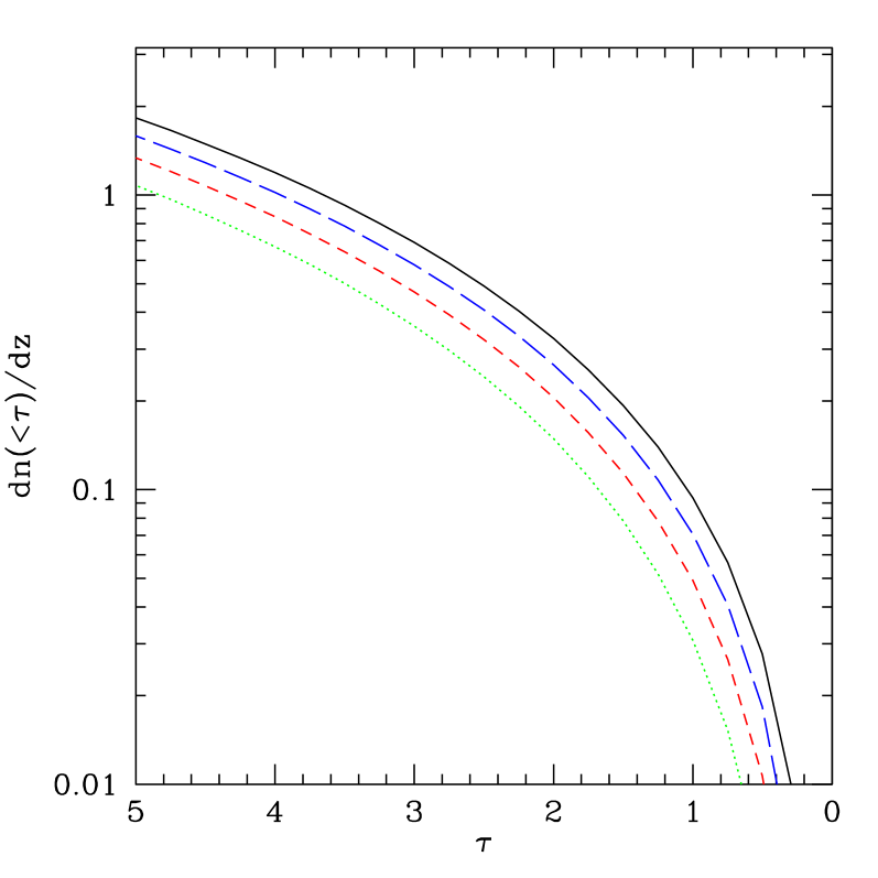
Figure 9: The expected number of transmission gaps at $z=6.1$ if the universe has $\bar{x}_{H}=0.1,\,0.15,\,0.2$, and $0.25$ (solid, long-dashed, short-dashed, and dotted curves, respectively). We have used the inhomogeneous IGM model described in §4.3 to construct the curves.

We caution the reader against overinterpreting these results. Uncertainties about the true distribution of sources and the density structure of the IGM make a quantitative comparison difficult at present (especially with the small observational sample). Moreover, our model probably begins to break down near overlap: by this point, the bubbles are so large that small scale structure and Lyman-limit systems will play an important role in determining the ionizing background.

Finally, the same quasar spectrum shows other Ly$\beta$ transmission gaps that could be compared to our model. However, the line of sight also contains a CIV absorber at $z=4.93$, and some of these spikes are likely emission lines from the same system (White et al., 2003). More data about which gaps are truly due to the interloper are crucial for extracting the most information possible from this spectrum.

5 Discussion

We have considered two methods to study the topology of reionization through near-infrared observations of high-redshift sources. The most promising technique is to measure the effects of damping wing absorption on the Ly$\alpha$ emission lines of high-redshift galaxies. Narrowband searches for galaxies with strong lines are one useful technique, and these surveys currently extend to $z\sim 6.5$ (e.g., Hu et al. 2002; Kodaira et al. 2003; Rhoads et al. 2004; Stanway et al. 2004b; Santos et al. 2004). They become increasingly difficult at higher redshifts because of the sky background, but some narrow transmission windows do remain in the near-infrared, and we expect high-redshift galaxies to have strong intrinsic Ly$\alpha$ lines (e.g., Partridge & Peebles 1967; Barton et al. 2004). Of course, the technique need not rely on galaxies selected in this way and can be applied to broadband photometric dropouts (e.g., Stanway et al. 2004a) as well as more specialised selection techniques (e.g., gravitational lensing, Kneib et al. 2004; Pelló et al. 2004).

Our results have several implications for such surveys. First, Ly$\alpha$ selection should be able to extend to eras well before reionization. Although at these times many galaxies will suffer significant damping wing absorption, reducing the apparent strength of their Ly$\alpha$ emission lines, a substantial fraction of galaxies will sit inside of large HII regions that allow transmission of a significant amount of flux in the Ly$\alpha$ line even when $\bar{x}_{H}\sim 0.75$. We thus expect that the number density of narrowband-selected galaxies will decline with redshift but that they will not disappear entirely. Second, because of the wide variance in IGM absorption for galaxies with the same intrinsic properties, we find that a single galaxy cannot provide tight constraints on either the ionization state of the IGM or the properties of the host galaxy (Hu et al., 2002; Rhoads et al., 2004; Loeb et al., 2004; Ricotti et al., 2004; Cen et al., 2004). Including the galaxy’s neighbors can make a dramatic difference to the expected level of inferred absorption. For example, massive galaxies at $z=6.5$ have a $\ga 20\%$ probability of sitting in HII regions with $\tau_{\rm damp}<2$ even if $\bar{x}_{H}=0.5$. Fortunately, the most massive galaxies generally dominate their local HII regions, so in that case such inferences will not be as dangerous (see Figure 3). Finally, our model also shows that cosmic variance in Ly$\alpha$-selected surveys will be even greater than expected, because the local overdensity of galaxies modulates the damping wing absorption (see Figure 4). We predict that, although some galaxies remain visible if $\bar{x}_{H}\la 0.5$, they are confined to increasingly rare regions of the universe.

On the other hand, the wide range of damping wing absorption expected through the middle ranges of reionization allows us to constrain the size distribution of HII regions during this era. This in turn will teach us about the properties of both the IGM and the high-redshift sources. Interestingly, because partial uniform reionization (such as from X-rays; Oh 2001; Venkatesan et al. 2001) and double reionization (e.g., Wyithe & Loeb 2003; Cen 2003b; Haiman & Holder 2003) affect the bubble sizes, such surveys can also help to constrain these models. Ideally, such a survey would use galaxies that are not selected through narrow-band imaging to avoid the selection effect described above, but for the time being Ly$\alpha$ line surveys look to be the most promising technique (at least for large cosmological volumes). Of course, we must separate the damping wing absorption from a variety of other complications, including gas infall, small-scale clumpiness, and galactic winds (Santos, 2004) before strong constraints can be made. With large samples, this should not be too difficult because we do not expect these local features to differ substantially across the large-scale environments that determine the topology of ionized bubbles.

A related technique is to measure the damping wing absorption from a gamma-ray burst afterglow (Miralda-Escude, 1998; Barkana & Loeb, 2004). The advantage of these objects is that their smooth power-law spectra (and lack of Ly$\alpha$ emission lines) makes interpreting the damping wing much simpler. Follow-up spectroscopy could then measure the host galaxy’s redshift and comparison to the damping wing would yield the size of the HII region. These host galaxies would be selected in an unbiased manner relative to the Ly$\alpha$ absorption, which would make their interpretation easier.

Of course, our model is only approximate. Numerical simulations are required to address questions such as the anisotropy of HII regions, the resonant absorption, and the effects of peculiar velocities. Gnedin & Prada (2004) have already made some steps in this direction; however, our model suggests that their box (with size $8h^{-1}$ comoving Mpc) is probably too small to obtain precise measurements, and in any case they were only able to examine one specific reionization history.

A second method to study the topology of reionization is to examine high-resolution quasar absorption spectra, which could contain gaps in the Gunn-Peterson trough when the line of sight passes close to the center of a large HII region. Previous studies had suggested that the strong damping wing absorption by the surrounding neutral IGM makes such gaps extremely rare. We have shown that the clustering of high-redshift galaxies makes the ionized bubbles much larger than naively expected, reducing the contribution of the damping wing. In this case, gaps are still expected to be rare because residual neutral gas (even with $x_{H}\sim 10^{-5}$) can provide substantial resonant absorption; late in reionization we expect $dn/dz\sim 0.02$–$0.3$ for features with $\tau<2$. However, weak transmission gaps are not so rare that their presence automatically implies an earlier episode of reionization. In particular, the gap at $z=6.08$ in the spectrum of SDSS J1148+5251 (White et al., 2003) does not necessarily imply an earlier overlap epoch (though of course it is consistent with such a scenario). It is encouraging that existing and near-future observations can help to constrain the topology of reionization. Because this technique relies on active ionizing sources to eliminate the resonant absorption, it is not terribly sensitive to complex reionization histories (which mostly affect the damping wing). Large HII regions already reduce the damping wing to manageable levels. Instead quasar absorption spectra are most sensitive to the instantaneous ionizing rate. We have also shown that the number of transmission gaps is nearly independent of the clustering and burstiness of ionizing sources. However, the widths of the gaps do vary with these quantities, so measurements of their sizes will help to constrain these parameters.

The principal source of uncertainty in this calculation is the inhomogeneous density distribution of the IGM, which we have accounted for only approximately. Unfortunately, the clumpiness of the IGM is difficult to quantify analytically. Numerical simulations can do much better, but we note that resolving the small scale density structure is particularly difficult in this case because the transmission gaps occur in the rare, large HII regions with sizes $\ga 10\mbox{ Mpc}$ (comoving). A complete solution would therefore require a large box and high mass resolution. Moreover, our model for the HII regions is only approximate and breaks down somewhat before overlap, once the mean free path of a photon is determined not by the bubble size but by small-scale overdensities (i.e., Lyman-limit systems). The topology of reionization during this era is best addressed through numerical simulations.

We also note that transmission gaps can occur if the line of sight passes near to a bright quasar (Miralda-Escude, 1998; Miralda-Escudé et al., 2000). Quasars produce such strong ionizing radiation fields ($\dot{N}_{\gamma}\ga 10^{57}$ photons s^-1 for the bright SDSS quasars, assuming the Elvis et al. 1994 template spectrum) that $\tau_{\rm res}$ is small within several comoving Mpc of the quasar. Estimates of the number density of gaps are difficult because they depend on the unknown luminosity function of fainter quasars. The best current estimate for quasars with $M_{1450}<26.7$ is $n_{\rm QSO}\sim 6\times 10^{-10}\mbox{ Mpc${}^{-3}$}$ at $z\sim 6$ (Fan et al., 2004). For these quasars, we then have $dn/dz\sim 10^{-4}$ for $\tau\la 1$ even if we neglect damping wing absorption. Thus the currently observed population should provide a negligible number of intersections. Extrapolating to fainter quasars is dangerous given the lack of observational constraints; however, if the luminosity function has a power law slope $\beta\sim-3$ (Fan et al., 2004) at the bright end, this steep component would have to extend to quasars a factor of $>100$ fainter than the observed population in order for gaps due to quasars to become comparable to our predictions for $\bar{x}_{H}<0.3$. This would require the break luminosity to occur at significantly smaller luminosities than observed at $z\sim 2$ (Boyle et al., 2000). Note also that the number density of quasars declines rapidly with redshift (it drops by a factor $\sim 30$ from $z=3$ to $z=6$; Fan et al. 2004), so quasars likely become even less significant at higher redshifts. Finally, because quasar HII regions are so large, the gradients in resonant absorption are relatively gentle and gaps near quasars should be quite wide in velocity space.

In summary, we find that both detailed studies of the absorption suffered by the Ly$\alpha$ emission lines of star-forming galaxies and searches for transmission gaps in the spectra of high-redshift quasars will enable us to constrain the size distribution of HII regions in the middle and late stages of reionization. Both of these methods are already able to probe the tail end of reionization at $z\sim 6$, and future surveys hold great promise to teach us even more.

This work was supported in part by NSF grants ACI AST 99-00877, AST 00-71019, AST 0098606, and PHY 0116590 and NASA ATP grants NAG5-12140 and NAG5-13292 and by the David and Lucille Packard Foundation Fellowship for Science and Engineering.

References

- Barkana (2002) Barkana R., 2002, New Astronomy, 7, 85
- Barkana (2004) Barkana R., 2004, MNRAS, 347, 59
- Barkana & Loeb (2001) Barkana R., Loeb A., 2001, Phys. Rep., 349, 125
- Barkana & Loeb (2002) Barkana R., Loeb A., 2002, ApJ, 578, 1
- Barkana & Loeb (2003) Barkana R., Loeb A., 2003, ApJ, submitted, (astro-ph/0310338)
- Barkana & Loeb (2004) Barkana R., Loeb A., 2004, ApJ, 601, 64
- Barton et al. (2004) Barton E. J., et al., 2004, ApJ, 604, L1
- Becker et al. (2001) Becker R. H., et al., 2001, AJ, 122, 2850
- Bond et al. (1991) Bond J. R., Cole S., Efstathiou G., Kaiser N., 1991, ApJ, 379, 440
- Boyle et al. (2000) Boyle B. J., et al., 2000, MNRAS, 317, 1014
- Bromm et al. (2001) Bromm V., Kudritzki R. P., Loeb A., 2001, ApJ, 552, 464
- Cen (2003a) Cen R., 2003a, ApJ, 597, L13
- Cen (2003b) Cen R., 2003b, ApJ, 591, L5
- Cen et al. (2004) Cen R., Haiman Z., Mesinger A., 2004, ApJ, submitted, (astro-ph/0403419)
- Ciardi et al. (2003) Ciardi B., Stoehr F., White S. D. M., 2003, MNRAS, 343, 1101
- Elvis et al. (1994) Elvis M., et al., 1994, ApJS, 95, 1
- Fan et al. (2002) Fan X., et al., 2002, AJ, 123, 1247
- Fan et al. (2003) Fan X., et al., 2003, AJ, 125, 1649
- Fan et al. (2004) Fan X., et al., 2004, AJ, in press, (astro-ph/0405138)
- Furlanetto et al. (2004a) Furlanetto S. R., Zaldarriaga M., Hernquist L., 2004a, ApJ, submitted (astro-ph/0404112)
- Furlanetto et al. (2004b) Furlanetto S. R., Zaldarriaga M., Hernquist L., 2004b, ApJ, submitted (astro-ph/0403697)
- Gnedin & Prada (2004) Gnedin N. Y., Prada F., 2004, ApJ, submitted, (astro-ph/0403345)
- Gunn & Peterson (1965) Gunn J. E., Peterson B. A., 1965, ApJ, 142, 1633
- Haiman (2002) Haiman Z., 2002, ApJ, 576, L1
- Haiman & Holder (2003) Haiman Z., Holder G. P., 2003, ApJ, 595, 1
- Holder et al. (2003) Holder G. P., Haiman Z., Kaplinghat M., Knox L., 2003, ApJ, 595, 13
- Hu et al. (2002) Hu E. M., et al., 2002, ApJ, 568, L75
- Hui & Haiman (2003) Hui L., Haiman Z., 2003, ApJ, 596, 9
- Kneib et al. (2004) Kneib J., Ellis R. S., Santos M. R., Richard J., 2004, ApJ, 607, 697
- Kodaira et al. (2003) Kodaira K., et al., 2003, PASJ, 55, L17
- Kogut et al. (2003) Kogut A., et al., 2003, ApJS, 148, 161
- Lacey & Cole (1993) Lacey C., Cole S., 1993, MNRAS, 262, 627
- Leitherer et al. (1999) Leitherer C., et al., 1999, ApJS, 123, 3
-
Loeb
et al. (2004)
Loeb A., Barkana R., Hernquist L., 2004, ApJ, submitted,
(astro-ph/0403193) - Madau et al. (1997) Madau P., Meiksin A., Rees M. J., 1997, ApJ, 475, 429
- Madau & Rees (2000) Madau P., Rees M. J., 2000, ApJ, 542, L69
- Miralda-Escudé et al. (2000) Miralda-Escudé J., Haehnelt M., Rees M. J., 2000, ApJ, 530, 1
- Miralda-Escude (1998) Miralda-Escude J., 1998, ApJ, 501, 15
- Oh (2001) Oh S. P., 2001, ApJ, 553, 499
- Partridge & Peebles (1967) Partridge R. B., Peebles P. J. E., 1967, ApJ, 147, 868
- Pelló et al. (2004) Pelló R., et al., 2004, A&A, 416, L35
- Press & Schechter (1974) Press W. H., Schechter P., 1974, ApJ, 187, 425
- Rhoads et al. (2004) Rhoads J., et al., 2004, ApJ, in press, (astro-ph/0403161)
- Rhoads & Malhotra (2001) Rhoads J. E., Malhotra S., 2001, ApJ, 563, L5
- Ricotti et al. (2004) Ricotti M., Haehnelt M. G., Pettini M., Rees M. J., 2004, MNRAS, submitted, (astro-ph/0403327)
- Santos et al. (2003) Santos M. G., et al., 2003, ApJ, 598, 756
- Santos (2004) Santos M. R., 2004, MNRAS, 349, 1137
- Santos et al. (2004) Santos M. R., et al., 2004, ApJ, 606, 683
- Scott & Rees (1990) Scott D., Rees M. J., 1990, MNRAS, 247, 510
- Shapiro et al. (2004) Shapiro P. R., Iliev I. T., Raga A. C., 2004, MNRAS, 348, 753
- Sheth (1998) Sheth R. K., 1998, MNRAS, 300, 1057
- Sheth & Diaferio (2001) Sheth R. K., Diaferio A., 2001, MNRAS, 322, 901
- Sokasian et al. (2002) Sokasian A., Abel T., Hernquist L., 2002, MNRAS, 332, 601
- Sokasian et al. (2003) Sokasian A., Abel T., Hernquist L., 2003, MNRAS, 340, 473
- Sokasian et al. (2003) Sokasian A., Abel T., Hernquist L., Springel V., 2003, MNRAS, 344, 607
- Sokasian et al. (2003) Sokasian A., et al., 2003, MNRAS, submitted, (astro-ph/0307451)
- Songaila (2004) Songaila A., 2004, AJ, 127, 2598
- Spergel et al. (2003) Spergel D. N., et al., 2003, ApJS, 148, 175
- Springel & Hernquist (2003) Springel V., Hernquist L., 2003, MNRAS, 339, 312
- Stanway et al. (2004a) Stanway E. R., et al., 2004a, ApJ, 607, 704
- Stanway et al. (2004b) Stanway E. R., et al., 2004b, ApJ, 604, L13
- Theuns et al. (2002) Theuns T., et al., 2002, ApJ, 567, L103
- Venkatesan et al. (2001) Venkatesan A., Giroux M. L., Shull J. M., 2001, ApJ, 563, 1
- White et al. (2003) White R. L., Becker R. H., Fan X., Strauss M. A., 2003, AJ, 126, 1
- Wyithe & Loeb (2003) Wyithe J. S. B., Loeb A., 2003, ApJ, 588, L69
- Wyithe & Loeb (2004a) Wyithe J. S. B., Loeb A., 2004a, Science, submitted
- Wyithe & Loeb (2004b) Wyithe J. S. B., Loeb A., 2004b, , 427, 815
- Zaldarriaga (1997) Zaldarriaga M., 1997, Phys Rev D, 55, 1822
-
Zaldarriaga et al. (2004)
Zaldarriaga M., Furlanetto S. R., Hernquist L., 2004, ApJ, in
press,
(astro-ph/0311514)