NGC 604, the Scaled OB Association (SOBA) Prototype. I: Spatial Distribution of the Different Gas Phases and Attenuation by Dust

Abstract

We have analyzed HST and ground-based data to characterize the different gas phases and their interaction with the Massive Young Cluster in NGC 604, a Giant H II Region in M33. The warm ionized gas is made out of two components: a high-excitation, high-surface brightness H II surface located at the faces of the molecular clouds directly exposed to the ionizing radiation of the central Scaled OB Association; and a low-excitation, low-surface brightness halo that extends to much larger distances from the ionizing stars. The cavities created by the winds and SN explosions are filled with X-ray-emitting coronal gas. The nebular lines emitted by the warm gas experience a variable attenuation as a consequence of the dust distribution, which is patchy in the plane of the sky and with clouds interspersed among emission-line sources in the same line of sight. The optical depth at H$\alpha$ as measured from the ratio of the thermal radio continuum to H$\alpha$ shows a very good correlation with the total CO ($1\rightarrow 0$) column, indicating that most of the dust resides in the cold molecular phase. The optical depth at H$\alpha$ as measured from the ratio of H$\alpha$ to H$\beta$ also correlates with the CO emission but not as strongly as in the previous case. We analyze the difference between those two measurements and we find that $\lesssim 11\%$ of the H II gas is hidden behind large-optical-depth molecular clouds; we pinpoint the positions in NGC 604 where that hidden gas is located. We detect two candidate compact H II regions embedded inside the molecular cloud; both are within short distance of WR/Of stars and one of them is located within 16 pc of a RSG. We estimate the age of the main stellar generation in NGC 604 to be $\approx$ 3 Myr from the ionization structure of the H II region, a value consistent with previous age measurements. The size of the main cavity is smaller than the one predicted by extrapolating from single-star wind-blown bubbles; possible explanations for this effect are presented.

1 INTRODUCTION

Giant H II Regions (GHRs) constitute one of the most conspicuous type of objects in spiral and irregular galaxies at optical wavelengths. For example, the 30 Doradus nebula can be detected with the naked eye at a distance of 50 kpc and five GHRs in M101 have their own NGC number at a distance of 7.2 Mpc. GHRs are powered by Massive Young Clusters (MYCs) that include $10^{2}-10^{3}$ O and WR stars, as opposed to the few stars of this type encountered in regular H II regions. The advent of high-spatial resolution data has revealed that GHRs have complex structures and cannot be accurately modeled as simple Strömgren spheres centered on the ionizing cluster. The deposition of energy in the form of ultraviolet light, stellar winds, and supernova explosions and the complex initial distribution in mass and velocity of the ISM produce a spatial distribution of the warm ionized gas that is anything but spherically symmetric. The analysis of the best studied GHR, 30 Doradus, reveals that most of the optical nebular emission originates at the surface of a molecular cloud in those points where it is directly exposed to the UV flux from the central cluster. The molecular cloud is what remains from the original material that gave birth to the MYC and the resulting region of intense optical nebular emission is a relatively thin layer instead of a classical Strömgren sphere (Walborn et al., 2002; Rubio et al., 1998; Scowen et al., 1998). This near-bidimensional character of an H II region is also observed in other objects, from the low-mass Orion nebula (Ferland 2001 and references therein) to much more massive regions such as N11 in the LMC (Barbá et al., 2003). Another property shared by these objects is that a second thin layer, the Photo Dissociation Region (PDR), where the non-ionizing UV light transforms H₂ into atomic hydrogen, can be found sandwiched between the H II region and the molecular cloud (Hollenbach & Tielens, 1997).

The MYCs at the center of GHRs can be divided into two types: Super Star Clusters (SSCs) are organized around a compact ($1-3$ pc) core while Scaled OB Associations (SOBAs) lack such a structure and are more extended objects, with sizes larger than 10 pc (Maíz-Apellániz, 2001). The cores of some SSCs (e.g. 30 Doradus) are surrounded by extended halos that are themselves similar to SOBAs in terms of structure and number of stars. This distinction between SSCs and SOBAs is important for the long-term evolution of the cluster, since the extended character of the latter makes them highly vulnerable to disruption by tidal forces on time scales shorter than the age of the Universe. Therefore, only SSCs are likely to survive to become the globular clusters of the future (Fall & Rees, 1977). MYCs are expected to form in a time scale shorter than 10 Myr but some of the best-studied examples, such as 30 Doradus and N11, reveal that their stars are not completely coeval: several million years after the central regions have been formed, there is induced star-formation in their periphery, leading to the so-called two-stage starbursts (Parker et al., 1992; Walborn & Parker, 1992; Walborn et al., 1999).

The analysis of GHRs in galaxies experiencing strong episodes of star formation has been the basic tool for decades to understand the properties of starbursts and their interaction with the surrounding medium. In order to characterize GHRs correctly, one has to establish the balance between the ionizing UV flux produced by the stars and the flux of the Balmer lines emitted by the GHR. The former can only be obtained from the analysis of the stellar continua in the UV domain, where the extinction is strongest. The latter fluxes are also affected by extinction, and it has been known for a long time that a simple correction using the H$\alpha$/H$\beta$ flux ratio might underestimate the intrinsic fluxes, due to the complex geometry of the dust and the gas within the GHR (Caplan & Deharveng, 1986). Furthermore, attempts to study the extinction in starbursts using integrated data have discovered that, on average, the color excess $E(B-V)$ experienced by the stars is about half that experienced by the gas (Calzetti et al., 2000), therefore complicating even more the calculation of the balance between the ionizing photons and the observed nebular spectrum, and making it very difficult to derive the fraction of ionizing photons escaping from the GHR.

The main objective of this work is therefore to characterize the properties, distribution and interrelation between the stars, gas and dust components of GHRs, in order to understand how they affect the resulting spectral energy distributions at various wavelength ranges. To achieve this goal we started some years ago a program to analyze in detail nearby resolved GHRs. In this work we present the first results obtained on NGC 604, concerning the properties of its gas and dust phases.

NGC 604 is a Giant H II Region in M33, the third largest galaxy in the Local Group after M31 and the Milky Way, located at a distance of 840 kpc (Freedman et al., 2001) along a direction with low foreground extinction (González Delgado & Pérez, 2000). 30 Doradus and NGC 604 are the two largest GHRs in the Local Group. NGC 604 is powered by a MYC without a central core that contains $\gtrsim 200$ O and WR stars (Maíz-Apellániz, 2001; Hunter et al., 1996; Drissen et al., 1993). The MYC is located inside a cavity that has the kinematic profile of an incomplete expanding bubble. On the other hand, the brightest knots all have kinematic profiles that can be well characterized by single gaussians (Sabalisck et al., 1995; Maíz-Apellániz, 2000), a strong indication that the overall dynamics of the GHR is not yet dominated by the kinetic energy deposition by stellar winds and SN explosions (Tenorio-Tagle et al., 1996).

Given its proximity, size, low foreground extinction and structural/kinematical properties, NGC 604 constitutes an ideal object for our study. It can indeed be considered as the prototype Scaled OB Association. We have combined HST and ground-based data to characterize the Massive Young Cluster, the surrounding Interstellar Medium and the interaction between them. In this first article we present and discuss the properties of the GHR created by the SOBA and its relationship with the molecular and coronal gas and dust clouds in the region. We have used WFPC2/HST and ground-based data to characterize the spatial distribution of the optical nebular emission properties. We have complemented this information with published data at other wavelength ranges. In a subsequent paper we will analyze the properties of the individual massive stars in NGC 604 and its extinction using HST imaging and HST objective-prism spectroscopy, aiming to derive accurately the properties of the individual stars and their evolutionary state. This will allow to compare the ionizing flux being emitted in the region with the value derived in this work from the nebular emission, constraining so the fraction of ionizing photons potentially escaping the region without contributing to the ionization.

We present the observations and describe the data analysis in section 2. We describe the attenuation by dust experienced by the warm ionized gas in section 3 and its density and excitation structure in section 4. Finally, we discuss our results in section 5.

2 OBSERVATIONS AND DATA ANALYSIS

2.1 WHT Long-slit spectra

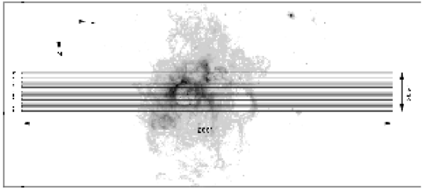
Figure 1: The ten long-slits superimposed on one of the F656N WFPC2 images. Note that north is towards the bottom and that this orientation is used throughout the article.

We obtained optical long-slit spectra of NGC 604 on the 18-19 August 1992 night with the ISIS spectrograph of the William Herschel Telescope as a part of the GEFE collaboration. The spectra were obtained at ten different positions, all of them at a P.A. of 90°, with an effective width for each one of 1″ and a spacing of $2\arcsec-3\arcsec$ between the center of each two consecutive positions (Fig. 1). Two spectra were taken simultaneously at each position, one in the range between 6390 Å and 6840 Å (red arm) and the other one in the range between 4665 Å and 5065 Å (blue arm), both of them with a dispersion of approximately 0.4 Å / pixel. The slit was approximately 200″ long, with a spatial sampling along the slit of 0$\farcs$33525 / pixel in the red arm and 0$\farcs$3576 / pixel in the blue arm. The exposure times ranged between 900 and 1200 seconds and the airmass varied between 1.21 and 1.01. More details of the data reduction and analysis are given in Maíz-Apellániz et al. (1998) and Maíz-Apellániz (2000).

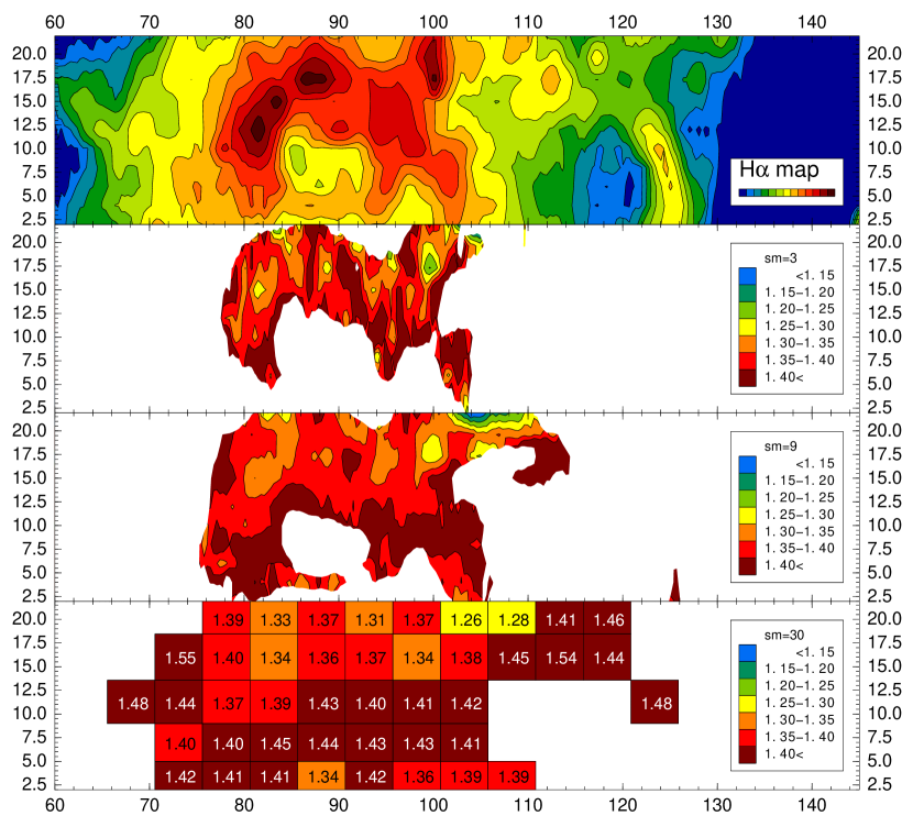
Figure 9: Synthetic H$\alpha$ map (top panel), density ratio maps (two middle panels), and density ratio table (bottom panel) produced from the long-slit data. The first density ratio map has been smoothed over 3 pixels (1″) along each slit while the second density ratio map has been smoothed over 9 pixels (3″). The color-coded density ratio table shows data averaged over 2 adjacent long slits and 15 pixels along the slit direction. In each of the lower three panels, data is shown where the uncertainty of the ratio is less than 0.08 in order to ensure that the values shown are relevant. The coordinates are expressed in arcseconds with north towards the bottom and east towards the right (see Fig. 1) with the first slit centered at $y=1\arcsec$ and its first pixel at $x=1/3\arcsec$. In these coordinates $(x,y)=(93\farcs 4,14\farcs 25)$ corresponds to ($1^{\rm h}\,34^{\rm m}\,33^{\rm s},\;30\arcdeg\,47\arcmin)$ in J2000.

With this strategy the direction perpendicular to the slit was under-sampled. However, taking into account that the seeing was comparable to the $1\arcsec-2\arcsec$ not sampled between subsequent slits, linear interpolation over the areas not covered is enough to reproduce the spatial distribution of the different parameters. This approach allowed us to cover the whole central region of NGC 604 in less than a single night without losing any significant amount of information. The reconstructed H$\alpha$ image (top panel in Fig. 9) shows indeed all the features obtained with imaging techniques at similar resolution. These data have been used for a variety of purposes in several previous works (Terlevich et al., 1996; Maíz-Apellániz, 2000; Tenorio-Tagle et al., 2000). Here we will use them to produce 2-D maps of the [S II] $\lambda$6717/[S II] $\lambda$6731 ratio across the face of NGC 604 and to calibrate the nebular WFPC2 data.

An additional set of spectroscopic data with the WHT were obtained by means of a spatial scan of the spectrograph perpendicular to the slit length direction, which was positioned at a PA=60°. These scanned spectra were centered at RA = 1^h 31^m 43^s, dec = 30° 31′52″, and they cover the core of the region by displacing a 1″-wide long-slit in steps of 1″ and taking at each position a 1 minute exposure. The details of this observation and of its calibration are given in González Delgado & Pérez (2000).

2.2 WFPC2 imaging

We list in Table 1 all the NGC 604 WFPC2 data currently available in the HST archive. The data correspond to four different programs, each with a different field of view, but all images include the region where the nebular line emission caused by the NGC 604 central cluster can be clearly identified. The images available in each program can be summarized as follows: 5237, optical broad-band ($UVI$) + H$\alpha$; 5384, FUV broad-band; 5773, “standard” narrow-band ([O III] $\lambda$5007, H$\alpha$, and [S II] $\lambda$6717+6731) + wide Strömgren $y$; and 9134, “extended” narrow-band ([O II] $\lambda$3726+3729, H$\beta$, [N II] $\lambda$6584, and [S III] $\lambda$9531). Only some of those images will be used in this paper but the common part of the reduction process is described here in order to use the data in a subsequent paper.

Table 1: NGC 604 WFPC2 data available in the HST archive.

Prog.	P.I.	Filter	Band	Data sets	Exp. times (s)
5237	Westphal	F336W	WFPC2 $U$	u2ab0207t + 208t	600 + 600
		F555W	WFPC2 $V$	u2ab0201t + 202t	200 + 200
		F814W	WFPC2 $I$	u2ab0203t + 204t	200 + 200
		F656N	H$\alpha$	u2ab0205t + 206t	1 000 + 1 000
5384	Waller	F170W	Far UV	u2c60b01t + 202t	350 + 350
5773	Hester	F502N	[O III] $\lambda$5007	u2lx0305t + 306t	1 100 + 1 100
		F656N	H$\alpha$	u2lx0301t + 302t	1 100 + 1 100
		F673N	[S II] $\lambda$6717+6731	u2lx0303t + 304t	1 100 + 1 100
		F547M	Wide Strömgren $y$	u2lx0307t + 308t	500 + 500
9134	Garnett	F375N	[O II] $\lambda$3726+3729	u6cj0201m + 202r +	2 700 + 2 700 +
				203m + 301m	2 700 + 2 700
		F487N	H$\beta$	u6cj0101m + 102m + 103m	2 700 + 2 700 + 2 700
		F658N	[N II] $\lambda$6584	u6cj0104m + 105m	1 300 + 1 300
		F953N	[S III] $\lambda$9531	u6cj0401m + 402m + 403m +	1 300 + 1 300 + 1 300 +
				404m + 405m + 406m	1 300 + 1 300 + 1 300

The standard WFPC2 pipeline process takes care of the basic data reduction (bias, dark, flat field corrections). Cosmic rays were eliminated in each case using the crrej task and the correction of the geometrical distortion and montage of the four WFPC2 fields was processed using the wmosaic task, both of which are included in the standard STSDAS package for WFPC2 data analysis. Hot pixels were eliminated using a custom-made IDL routine.

The next step in the data reduction, the registering of the images obtained under different programs, followed a more elaborated process. The geometric distortion of the WFPC2 detectors is well known (Casertano & Wiggs, 2001), allowing for a precise relative astrometry. However, the absolute astrometry has two problems: First, the Guide Star Catalog, which is used as a reference, has typical errors of $\sim 1\arcsec$ (Russell et al., 1990). Second, if only one point in one of the four WFPC2 chips can be established as a precise reference using an external catalog, the average error in the orientation induces an error of $\sim 0\farcs 03$ in a typical position in the other three chips. In our case, a star that is present in all 13 WFPC2 fields is included in the Tycho-2 catalog as entry 2 293-642-1. We used the VizieR service (Ochsenbein et al., 2000) to obtain its coordinates and proper motion using the J2000 epoch and equinox and we then corrected for the different epoch of the observations. The star is saturated (in some filters only weakly, with only a few pixels affected, but in others quite heavily, with significant bleeding to pixels in the same column) in all filters except F170W but we were able to fix its centroid within one quarter of a WF pixel in all cases using the diffraction spikes. Thus, the procedure followed to establish a uniform coordinate system had three steps. First, we corrected for the difference in plate scale for each filter with respect to F555W using the parameters provided by Dolphin (2000). Note that at the present time the STSDAS tasks wmosaic and metric use the non-wavelength-dependent Holtzmann solution, which can introduce $\sim 0\farcs 1$ errors for FUV data; errors are an order of magnitude or less smaller if only optical data are involved. Second, we rotated all mosaiced images in order to make them share a common orientation. Third, using TYC 2 293-642-1 as a reference, we corrected for the general displacement in RA and declination and compared the positions of the stars in the central region of NGC 604 (at a distance of $\sim 70\arcmin$) using images obtained under different filters. As expected, coordinates differed by a few hundredths of an arcsecond, which we take to be the precision of our absolute astrometry.

In this first paper we are interested in obtaining “pure nebular” H$\alpha$, H$\beta$, [O III] $\lambda$5007, [N II] $\lambda$6584  and [S II] $\lambda$6717+6731 images from the narrow-band F656N, F487N, F502N, F658N, and F673N WFPC2 data, respectively. In order to do that, we used the broad-band images to eliminate the continuum contribution. Following this approach one has to be careful since broad-band images can be contaminated by the nebular emission itself (this is especially so for F555W data). If one has to use a heavily-contaminated broad-band filter to subtract the continuum, the full linear system of equations for the reciprocal contributions has to be solved (see, e.g. MacKenty et al. 2000). Here we used F814W, F547M, and F336W images, which have much weaker nebular contaminations and can be considered to a first order approximation as free from contributions from emission lines. The continuum at H$\alpha$, [N II] $\lambda$6584, and [S II] $\lambda$6717+6731 was interpolated from the F547M and F814W data while that of H$\beta$ and [O III] $\lambda$5007 was interpolated from the F336W and F547M data. In principle, the continuum subtraction for the first three lines is expected to be more accurate than for the last two for two reasons: (1) The difference in flux between F547M and F814W is relatively small for the type of sources that contribute to the continuum (early-type stars for the central cluster region, nebular continuum for the nebulosity, late-type stars for the background) in comparison to the difference in flux between F336W and F547M for some of those types. (2) Some of those source types have strong Balmer jumps in their spectra, which makes interpolation between F336W and F547M more inaccurate. With those caveats in mind, we tested several interpolation mechanisms and the best results (for both point sources and background) were obtained using a double (in $\lambda$ and in flux) logarithmic scale, which is exact if the flux follows a power law in $\lambda$. We should point out that, even though the remaining flux due to the continuum contribution at the location of a bright star in the final nebular image typically averages to zero (i.e. the overall continuum subtraction is correct), there is usually some structure visible at such locations in the resulting image. The main reason for this effect is the undersampled nature of the WFPC2 PSF, which does not permit a perfect subtraction of one image from another. For that reason, we decided to blank out in the nebular images those areas with bright stars and when measuring the integrated nebular fluxes we have interpolated in those regions using the neighboring pixels. Another issue related to the obtention of pure nebular images, the mutual contamination between H$\alpha$ and [N II] $\lambda$6548+6584 in the F656N and F658N filters is discussed later.

Another topic that needs to be addressed here is that of the absolute photometric calibration of the WFPC2 nebular filters. It is stated in the HST Data Handbook (STScI, 2002) that their accuracy is estimated to be $\lesssim 5\%$. A recent study by Rubin et al. (2002) found this to be true for three of the filters used here, F487N, F502N, and F656N (see Table 2). We performed an independent calibration of four of the nebular filters (F487N, F656N, F658N, and F673N) using the NGC 604 H$\alpha$ and H$\beta$ images published by Bosch et al. (2002), which were kindly made available to us by Guillermo Bosch, and our WHT long-slit spectra. For each filter we used synphot (STScI, 1999) to obtain the conversion factors between detector and physical units both for a continuum source and for an emission line with the appropriate blueshift corresponding to NGC 604.

1. For F487N, we compared the continuum-subtracted integrated flux over a $50\arcsec\times 50\arcsec$ region (after smoothing the image with a Moffat kernel to degrade its resolution) with the same value derived from the Bosch et al. (2002) data.

2. For F656N, we used a similar but more complex procedure. The photons detected in that filter can originate in the continuum, H$\alpha$ itself, or one of the neighbor [N ii] lines. Given that the expected ratios are rather low ([N II] $\lambda$6584/H$\alpha$$\sim$ 0.1, [N II] $\lambda$6548/H$\alpha$$\sim$ 0.03) and that the throughput peaks near the wavelength of H$\alpha$, the contamination by [N ii] is expected to be not too important ($<10\%$) but still significant. On the other hand, F658N is also contaminated by H$\alpha$ emission to a similar degree (H$\alpha$ falls at the tail of the filter throughput at the blueshift of NGC 604). Therefore, we decided to eliminate the mutual contamination by establishing the 2 linear equations with the coefficients determined from synphot and solving for the two unknowns, H$\alpha$ and [N II] $\lambda$6584, using [N II] $\lambda$6584/[N II] $\lambda$6548 = 3. We then compared the obtained H$\alpha$ flux with the Bosch et al. (2002) data in a manner analogous to what we did previously for H$\beta$.

3. To verify the calibration for F658N and F673N we first obtained the continuum-subtracted images (and for the case of F658N we also eliminated the H$\alpha$ contribution as detailed in the previous point) and degraded their resolution with a Moffat kernel. We then calibrated the H$\alpha$ fluxes from the long-slit spectra with the H$\alpha$ image from Bosch et al. (2002) after shifting the relative positions of the long-slits to match the structures seen in the corresponding cuts of the images. We used the absolute calibration thus provided to obtain the corresponding [N II] $\lambda$6584 and [S II] $\lambda$6717+6731 fluxes for the long-slit spectra and then compared the integrated fluxes with those obtained from the WFPC2 F658N and F673N data.

Given the mutual influence in the calibration of F656N and F658N, the above procedure was iterated several times until convergence was reached. The results are shown in Table 2 in the form of the ratio between the values of the EMFLX parameter (the factor used to convert from ADU/s to monochromatic flux) as provided by synphot and as measured here. For all four cases we detect that synphot slightly overestimates the throughput of the nebular filters, which is the same effect that was detected by Rubin et al. (2002) for two of them, F487N and F656N (they did not analyze F658N and F673N). Our values are similar but not identical, which is not unexpected given that the different radial velocities of the objects studied is sufficient to shift the wavelengths of the emission lines by several Angstroms. In the rest of this paper we will use the calibration discussed here for F487N, F656N, F658N, and F673N and the one obtained by Rubin et al. (2002) for F502N.

It should be noted that Charge Transfer Efficiency (CTE) effects are not included in the results of Table 2, either for the new values or for those extracted from Rubin et al. (2002), and that could be a major factor in the existing differences Since our data have been directly calibrated using ground-based fluxes (except for F502N) this should not be a problem for the results in this paper. However, one should be careful when using the results in Table 2 with other data and, if possible, should attempt a similar procedure as the one outlined in the previous paragraphs.

Table 2: Absolute flux calibration of the nebular WFPC2 filters. The quantity plotted in each case is the EMFLX parameter (conversion factor between count rate and monochromatic line flux) provided by synphot (STScI, 1999) divided by the value of EMFLX measured by alternative calibrations. A value greater than one indicates that synphot overstimates the throughput and, therefore, that the sense of the correction is to increase the line flux (since in that case a larger real count rate is necessary to produce a given monochromatic flux).

Data	F487N	F502N	F656N	F658N	F673N
synphot calibration	1.000	1.000	1.000	1.000	1.000
Table 1 of Rubin et al. (2002)	1.032	0.959	1.037	—–	—–
Bosch et al. (2002) data	1.012	—–	1.101	—–	—–
Bosch et al. (2002) + long-slits	—–	—–	—–	1.210	1.114

2.3 Other data

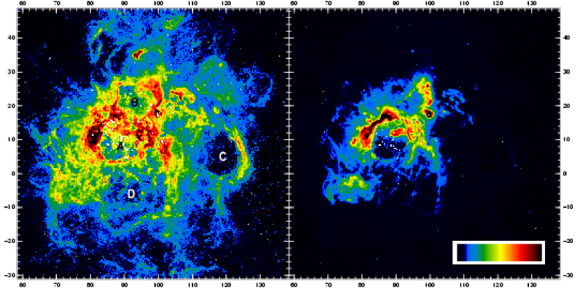
Figure 2: WFPC2 continuum-subtracted [S II] $\lambda$6717+6731 (left) and [O III] $\lambda$5007 (right) images. Both images are displayed with a hyperbolic intensity scale in order to show both low and high intensity structures. White pixels are used to block regions with bright stars for the sake of clarity (continuum subtraction is not perfect there due to the under-sampled nature of the WFPC2 PSF). The larger extension of the emission in the [S II] $\lambda$6717+6731 image as compared to that of the [O III] $\lambda$5007 is not an artifact of the choice of displayed levels. On the contrary, the dynamic range (defined as the ratio between maximum and minimum displayed levels) for the image on the left is 100 while that for the image on the right is 1 000. Therefore, if both lines were emitted from regions of similar size, one would expect the [O III] $\lambda$5007 region to appear larger instead of smaller. The letters A to D indicate the location of the four cavities described in the text. The field is 80″ on a side and the orientation is the same as in the rest of the figures. See Fig. 9 for an explanation of the coordinate system.

In order to provide a more complete picture of the ISM in NGC 604 we obtained some additional data from the literature and other archives. Ed Churchwell generously provided us with the data shown in Fig. 2 of Churchwell & Goss (1999). Those authors obtained a 3.6 cm radio continuum map of NGC 604 with the VLA and combined the data with a ground-based H$\alpha$ image of the region to produce a map of $\tau_{\rm rad}$, the (true) optical depth experienced by H$\alpha$ emission (see Appendix). Here we will use the $\tau_{\rm rad}$ map to compare it with a $\tau_{\rm Bal}$ map, that is, a map of the optical depth at H$\alpha$ as measured from the ratio of the fluxes of the H$\alpha$ and H$\beta$ emission lines. A vital step to do an study of the attenuation by dust is to obtain a correct registration between the images obtained at different wavelengths. In order to do this we first degraded the spatial resolution of our WFPC2 H$\alpha$ and H$\beta$ images in order to match that of the radio data. As it is discussed later in the paper, some of the bright H II knots are located on extinction gradients and this can cause a significant displacement between the positions of the intensity peaks in H$\alpha$ and radio, rendering those knots useless for registration purposes. Therefore, we decided to use instead for registration (a) the SNR present in NGC 604 (knot E in Churchwell & Goss 1999), which is located in a relatively dust-free area and should have the same coordinates in both the optical and radio data (D’Odorico et al., 1980; Gordon et al., 1998); and (b) the intensity minima determined by the cavities in the ionized gas, since those structures are also located on areas with low attenuation. This process yielded a registration correct to better than 0$\farcs$5 without requiring the use of a rotation between the optical and radio data, as estimated from the residuals in the fit. Given that the radio beam had a HPBW of $4\farcs 18\times 3\farcs 63$, the precision in the registering is good enough for our purposes.

We also extracted from the M33 CO ($1\rightarrow 0$) survey of Engargiola et al. (2003) a map of the NGC 604 region. That survey was obtained with BIMA and has a spatial resolution of 13″. Finally, we also retrieved from the Chandra archive a 90 ks image of NGC 604 obtained with ACIS (P.I.: Damiani). The X-ray data were registered to the optical data using the SNR in NGC 604. Here we will use the CO and X-ray data to compare the morphologies of the different phases of the ISM in NGC 604.

3 NEBULAR MORPHOLOGY AND ATTENUATION BY DUST

3.1 Nebular morphology

The nebular structure of NGC 604 consists of a central bright, high-excitation region surrounded by a dimmer low-excitation halo. The central region is detected in all bright nebular lines while the halo can be easily seen only in low-excitation lines such as [S II] $\lambda$6717+6731 or [N II] $\lambda$6584 (see Fig. 2). The high excitation region is composed of a $16\arcsec\times 14\arcsec$ shell surrounding a central cavity (which we will call A following the nomenclature of Maíz-Apellániz 2000) centered on coordinates (90″,9″); two filaments that extend N/S along $x=100\arcsec$ and $x=104\arcsec$, respectively; and a filled H II region centered at (76″,$-$5″).

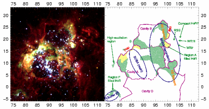
Figure 3: (left) Color mosaic of the central region of NGC 604 composed by assigning F673N to the red channel, F555W and F656N to the green one, and F336W to the blue one (the filters were not processed for continuum or line subtraction). The field is 39″ on a side and the orientation is the same as in the rest of the figures. See Fig. 9 for an explanation of the coordinate system. (right) Explanatory diagram for some of the structures discussed in the text. Violet is used to display cavity contours, with a dashed line style when the boundary between cavities is uncertain (possibly due to superbubble bursting), and shading is used to mark the high excitation parts of the nebula (H II surfaces), with yellow used for the regions with the highest intensity and green used for the rest.

The SOBA has two loosely-defined components, a main one centered at cavity A and elongated in the N-S direction (from approximately (92″,2″) to (85″,18″), see Fig. 3) and a secondary one, more dispersed and approximately cospatial with the eastern part of the shell around cavity A and the two high-excitation filaments located towards the E (in the range $x=92\arcsec-103\arcsec$ and $y=2\arcsec-25\arcsec$, see Fig. 3). Another more distant group of bright stars can be seen at the location of the filled H II region towards the NW (this group is called cluster B in Hunter et al. 1996).

The shell around cavity A is far from uniform. Towards the SW it is very bright and very thin (likely unresolved) in [O III] $\lambda$5007. Towards the E it is of intermediate brightness, much thicker and less well defined, with a bright intrusion extending towards the center of the cavity at (90″, 12″) (Tenorio-Tagle et al., 2000). Towards the N it is thin and well defined again but dimmer. The two eastern filaments are also not uniform, with the southern one brighter than the northern one. We want to stress that the optical appearance of all the high excitation regions is consistent with them being thin structures (thicknesses of $1-2$ pc), with an apparent variable thickness created by different inclinations with respect to the observer. As described in the introduction, this is the observed geometry for well-studied galactic and extragalactic H II regions. This effect is seen, for example, in that the areas with the highest surface brightness appear to be one-dimensional, as expected from orientation effects when the geometry is such that we observe the surface edge on. Later on, we describe other observational evidence that support this model for the structure of the H II gas in NGC 604.

Tenorio-Tagle et al. (2000) explored the kinematics of the H II gas in NGC 604 and found that the shell around cavity A can be characterized by a single gaussian profile with an approximately constant velocity of $-255$ km s^-1. The H II gas on cavity A itself needs to be described by at least two kinematic components, one shifted towards the red and one towards the blue. The red component is present everywhere and shows the spatial profile of an expanding bubble while the blue one has a patchy coverage. The bright intrusion at (90″, 12″) is part of the blue-shifted component. Tenorio-Tagle et al. (2000) interpreted this kinematic profile as a sign that the superbubble originally associated with cavity A had burst in the direction towards us.

Two other cavities are visible in the nebular-line images towards the S and N; we will call them B and D, respectively, following the previously established nomenclature (see Fig. 2). They contain only a few massive stars each. Their kinematics were partially mapped by Tenorio-Tagle et al. (2000) and they were found to be similar to that of cavity A: the walls have single gaussian components with approximately constant velocity while the cavity itself shows line-splitting indicative of expansion. Given the low number of massive stars these two structures contain and that they are apparently connected to the main cavity (there are regions at the boundaries where only weak low-excitation nebular emission can be seen), a likely origin for these two structures is that they were also produced by the superbubble in cavity A bursting out into the surrounding medium (in this case along the plane of the sky rather than along the line of sight).

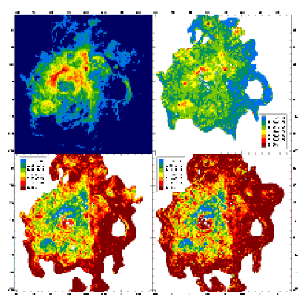
Figure 12: A continuum-subtracted H$\alpha$ WFPC2 image of NGC 604 is shown in the upper left panel. The other three panels show excitation maps of the same region: [O III] $\lambda$5007/H$\beta$ (upper right) [S II] $\lambda$6717+6731/H$\alpha$ (lower left), and [N II] $\lambda$6584/H$\alpha$ (lower right). Areas in white have been masked due to strong stellar contamination or low signal-to-noise. The field is the same as the one in Fig. 2. See Fig. 9 for an explanation of the coordinate system.

The region towards the E of the $x=100\arcsec-104\arcsec$ filaments is marked by a sharp drop in the excitation ratios (see Fig. 12). A fourth cavity (C) is centered on (119″,5″). It differs from the previous three in that the intensity of the nebular lines in its central region is weaker and does not show line splitting. Only a few stars are present inside and, judging from their magnitudes, they are likely to be of late-O or early-B type at most. All of this suggests that the fourth cavity is an older structure which has been recently re-ionized by the current burst.

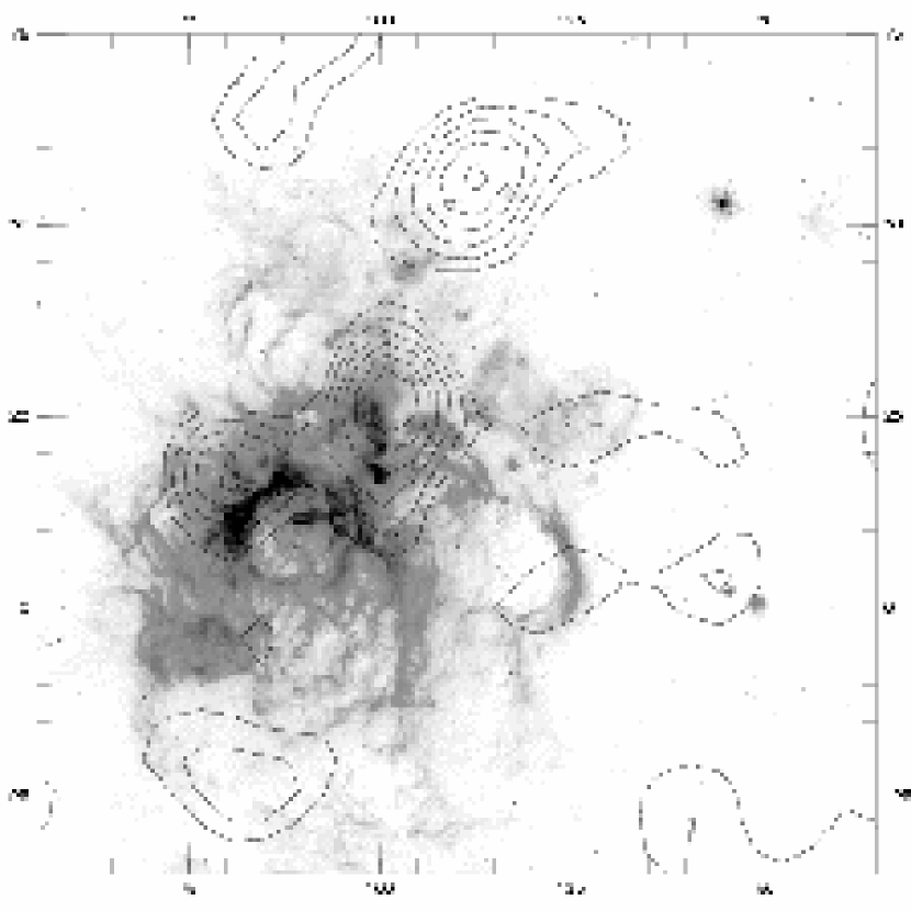
Figure 4: Contour diagram of the CO ($1\rightarrow 0$) emission in NGC 604 (adapted from the data of Engargiola et al. 2003) superimposed on an F656N WFPC2 image (without continuum subtraction). The spatial resolution of the contour diagram is 13″. The field is 110″ on a side and the orientation is the same as in the rest of the figures. See Fig. 9 for an explanation of the coordinate system.

The distribution of the CO ($1\rightarrow 0$) emission in NGC 604 with respect to the H II region is shown in Fig. 4. Two clouds can be seen close to the SOBA. The largest one is centered on (102″,27″) while the second one is centered on (80″,17″). Farther away, a third cloud is centered on (113″,51″) and a fourth, much less intense, on (82″,-23″). Looking at Fig. 4 and allowing for the difference in spatial resolution between the two data sets, it can be seen that all the bright areas of the H II region are (a) located at the edges of the first two molecular clouds and (b) oriented towards the ionizing sources. As we have already mentioned, this is the same configuration observed in Galactic H II regions and in more massive objects such as 30 Doradus and N11 and provides further evidence towards the near-2D character of these areas. Therefore, it appears to be a general configuration that the bright areas of H II regions (excepting maybe the oldest and the youngest ones) originate in the surface of molecular clouds directly exposed to massive young stars.

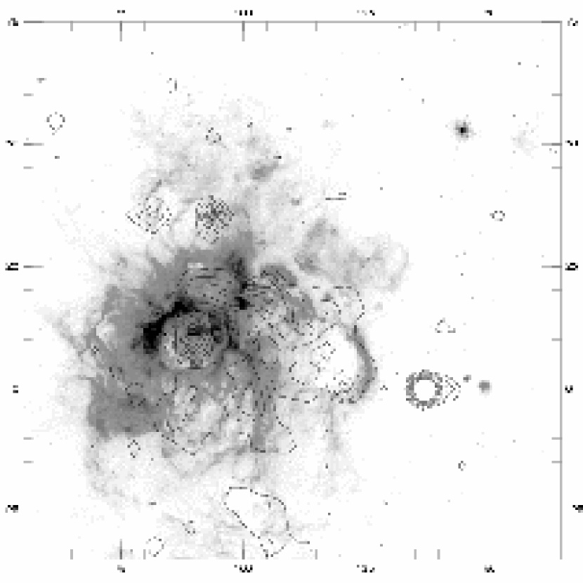
Figure 5: Contour diagram of the X-ray emission in NGC 604 superimposed on an F656N WFPC2 image (without continuum subtraction). The field and orientation is the same as in Fig. 4.

Diffuse X-rays are observed filling the four cavities in NGC 604 (see Fig. 5), with the highest intensity originating in the main one. Two point sources are also detected: one is the SNR and the other one, located at (137″,0″), is not associated with any of the other sources described in this paper. The integrated X-ray emission from the diffuse gas was modeled by Yang et al. (1996). The X-ray emission is very soft, with a best-fitting Raymond-Smith model with a plasma temperature of $1.3\times 10^{6}$ K ($kT=0.12$ keV), giving a luminosity in the 0.5–2 keV range of around $8\times 10^{38}$ erg s^-1. These authors concluded that the X-ray emission is most likely dominated by the contribution from a hot, thin plasma energized by stellar winds. Cerviño et al. (2002) predict a soft X-ray emission of around $10^{34}$ erg s^-1 M${}_{\odot}^{-1}$ for a MYC of 3 Myr, assuming average conditions. For a total stellar mass of around $10^{5}$ M_⊙ in the range 2–120 M_⊙ (Yang et al., 1996), we conclude that the observed X-ray luminosity is indeed consistent with a hot plasma energized by a young massive cluster. As discussed by Cerviño et al. (2002), the contribution by individual stars of any kind at this age should be only around $10^{30}$ erg s^-1 M${}_{\odot}^{-1}$, which is negligible in comparison with the contribution of the coronal gas.

3.2 Attenuation data

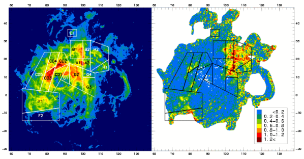
Figure 6: (Left) Continuum-subtracted H$\alpha$ WFPC2 image of NGC 604. (Right) $\tau_{\rm Bal}$ map of the same region as derived from WFPC2 data smoothed with a $5\times 5$ WF pixels box. Areas in white have been masked due to strong stellar contamination or low signal-to-noise. The sub-regions used in this paper are shown. The field is the same as the one in Fig. 2. See Fig. 9 for an explanation of the coordinate system.

We have smoothed our continuum-subtracted H$\alpha$ and H$\beta$ images with a $5\times 5$ pixel box, calculated their ratio, and applied Eq. 6 to obtain a map of $\tau_{\rm Bal}$, the optical depth at H$\alpha$ measured from the ratio of the two Balmer lines. The result is shown in Fig. 6, where we have masked out bright stars (as previously described) and areas with low values of the S/N ratio. We stress again the need for an accurate registering and flux calibration for such a map to be a realistic representation of $\tau_{\rm Bal}$, topics that we have covered in the previous section. Other aspects that require some words of caution regarding Fig. 6 are also detailed here:

• An incorrect temperature can induce systematic differences in the value of $\tau_{\rm Bal}$ (see Eq. 5 in the Appendix). For NGC 604 we use a value of 8 500 K based on the measurements of $8\,150\pm 150$ K for $T_{e}$([O III]) and $8\,600\pm 450$ K for $T_{e}$([N II]) of Esteban et al. (2002) (see also Díaz et al. 1987; González Delgado & Pérez 2000). However, the temperature dependence is rather weak: a change from 8 500 K to 10 000 K (which is too large to be realistic for NGC 604, see Díaz et al. 1987; Esteban et al. 2002) changes $\tau_{\rm Bal}$ only from 0.245 to 0.273 for $F_{\alpha}/F_{\beta}=3.2$. The dependence is stronger for the case of $\tau_{\rm rad}$ (see Eq. 2) but the uncertainties introduced by a possible error in the temperature are not large. A change from 8 500 K to 10 000 K would change the overall value of $\tau_{\rm Bal}$ for NGC 604 only from 0.54 to 0.63.

• The existence of scattered Balmer radiation from a dust cloud can yield localized values of $F_{\alpha}/F_{\beta}$ lower than the canonical value corresponding to $\mbox{$\tau_{\rm Bal}$}=0$. Such a phenomenon has been observed in e.g. NGC 4214 (Maíz-Apellániz et al., 1998) and it is also present here in a few pixels in the central cavity. In those cases we have simply used $\mbox{$\tau_{\rm Bal}$}=0$.

Our $\tau_{\rm Bal}$ map provides us with a 0$\farcs$5 (2 pc) resolution map of the attenuation experienced by the H II gas in NGC 604. The problem of recovering the flux lost by geometrical effects in the dust distribution (as opposed to the flux lost by the total amount of dust present between the source and the observer) can be divided into two parts: (a) the patchiness of the dust geometry in the plane of the sky and (b) the possibility that some of the dust may be interspersed among sources along the same line of sight. (a) has the effect of underestimating the real H$\alpha$ flux. If we have observations with a spatial resolution comparable to the scales in which the dust distribution varies, then we can correct for the effects of dust by applying an extinction correction pixel by pixel. This is the main motivation for producing a $\tau_{\rm Bal}$ map with the highest possible spatial resolution.

The solution to (b) is more complicated. Suppose we have a thick dust cloud located between sources A and B, both in the same line of sight with A closer to the observer. In that case, most or all of the Balmer photons emitted from B will be absorbed in the cloud and our value of $\tau_{\rm Bal}$ will be only a measurement of the possible foreground extinction experienced by A. From the point of view of H$\alpha$ and H$\beta$ the existence of B will be unknown to us and if we were to estimate the ionizing flux from that information, we would miss the contribution from B completely. In a general case, it can be shown that the effect of (b) is the same as that of (a): to introduce an underestimation of the total ionizing flux. What can we do to recover the lost flux? One solution is to use the thermal radio continuum, which is unaffected by dust and can give us a better estimate of the ionizing flux. Nevertheless, there are two considerations that affect radio observations:

• At the present time, radio observations of low-to-medium emission-measure thermal sources such as extragalactic H II regions have lower spatial resolution than that available from optical observations. The VLA can reach HST-like resolution but only for high emission-measure sources.

• It is possible to have contamination from non-thermal continuum radio sources such as SNRs. This can be mitigated by observing at multiple wavelengths but such a procedure can introduce large uncertainties if the non-thermal contribution is large.

In addition, a fraction of the ionizing photons might simply be destroyed by dust and/or might escape the region without contributing to the ionization process. In our next paper we will characterize the massive stellar population and will compare the predicted with the measured fluxes, aiming to constrain the fraction of escaping photons.

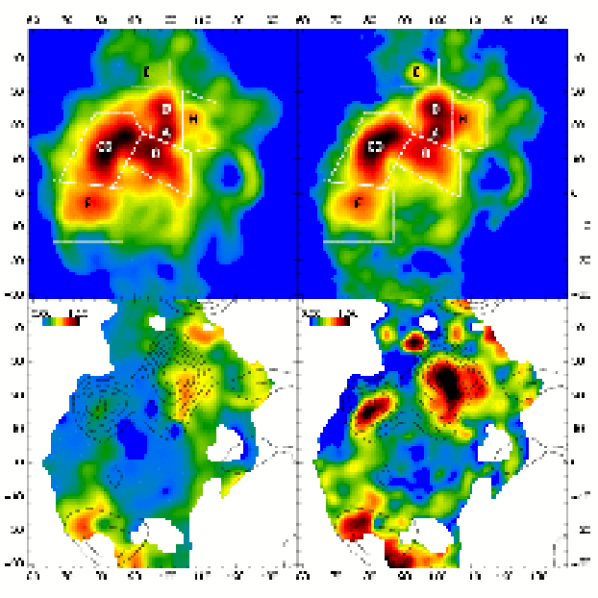
Figure 7: (Upper left) Low ($\approx 4\arcsec$) resolution continuum-subtracted H$\alpha$ image of NGC 604. (Upper right) 8.4 GHz radio continuum image of NGC 604 at the same resolution. (Lower left) $\tau_{\rm Bal}$ map of the same region at that resolution. (Lower right) $\tau_{\rm rad}$ map of the same region at that resolution. The regions used in this paper are shown in the upper two panels. Areas in white in the two lower panels have been masked due to low signal-to-noise. Contours from the CO data shown in Fig. 4 are plotted in the lower two panels. The field is the same as the one in Fig. 2. See Fig. 9 for an explanation of the coordinate system.

In order to explore the relative importance of the non-uniform dust distribution in the plane of the sky and along the line of sight we have produced an $\approx 4\arcsec$ resolution map of $\tau_{\rm rad}$, the real optical depth at H$\alpha$ as measured from the ratio of the thermal radio continuum to H$\alpha$ (see Eq. 3 in the Appendix). The map is shown in Fig. 7 along with the original radio image, the resolution-degraded WFPC2 H$\alpha$ image used to calculate $\tau_{\rm rad}$, and a $\tau_{\rm Bal}$ map at the same resolution and scale as the $\tau_{\rm rad}$ one. We have also integrated the fluxes along the polygonal regions shown in that same figure, which correspond to the main H II knots, and have computed the corresponding values of $\tau_{\rm rad}$ and $\tau_{\rm Bal}$ (see Table 3). In that same table we include three other quantities. The first one, $\tau^{\prime}_{\rm Bal}$, is the value of $\tau_{\rm Bal}$ calculated by correcting for extinction pixel by pixel in the region using the full-resolution WFPC2 images, i.e. the weighted value we recover by using the spatial information in the plane of the sky up to the resolution provided by WFPC2. One expects that $\mbox{$\tau_{\rm Bal}$}<\mbox{$\tau^{\prime}_{\rm Bal}$}<\mbox{$\tau_{\rm rad}$}$, since $\tau^{\prime}_{\rm Bal}$ does not correct for structures present in the dust at smaller spatial scales and along the line of sight, and that is indeed the case for all entries in Table 3. The other two quantities are the values of $\tau_{\rm cov}$ and $\gamma$ corresponding to $\tau_{\rm rad}$ and $\tau_{\rm Bal}$ applying the patchy foreground model of the Appendix and using the one-to-one mapping that can be derived from Fig. 8.

Table 3: Integrated values for A to H regions.

Apert.	Area	$F_{\rm rad}$	$F_{\alpha}$	$F_{\rm rad}/F_{\alpha}$	$\tau_{\rm rad}$	$F_{\beta}$	$F_{\alpha}/F_{\beta}$	$\tau_{\rm Bal}$	$\tau^{\prime}_{\rm Bal}$	$\tau_{\rm cov}$	$\gamma$
A	48.80	3.62	13.73	0.264	0.92	4.12	3.330	0.34	0.47	2.02	0.695
B	116.39	6.55	20.96	0.313	1.09	6.24	3.357	0.36	0.45	2.27	0.741
CD	347.47	17.92	87.71	0.204	0.67	28.13	3.118	0.18	0.25	2.17	0.549
E	93.96	0.67	3.48	0.192	0.61	1.07	3.258	0.29	0.51	1.48	0.588
F	349.04	4.82	29.35	0.164	0.45	9.05	3.244	0.28	0.40	1.03	0.561
G	208.20	6.90	47.22	0.146	0.33	15.71	3.006	0.09	0.21	1.89	0.333
H	161.82	3.29	11.09	0.297	1.04	2.92	3.798	0.66	0.80	1.52	0.827
A-H	1325.68	43.78	213.55	0.205	0.67	67.25	3.176	0.23	0.34	1.92	0.572
NGC 604	6120.94	56.77	314.60	0.180	0.54	99.17	3.172	0.22	0.42	1.59	0.525
NGC 604 (no E)	6026.98	56.10	311.12	0.180	0.54	98.10	3.172	0.22	0.41	1.59	0.525

Note. — The two largest uncertainty sources for the optical depths are the absolute flux calibration and the assumed temperature. See the discussion in subsections 2.2 (see Table 2) and 3.2, respectively.

In order to make better use of the high-resolution optical data, we have subdivided the A to H regions into sub-regions and calculated the corresponding values of $\tau_{\rm Bal}$ and $\tau^{\prime}_{\rm Bal}$. The results are shown in Table 4, where the entry “diffuse” refers to the totality of the integrated area except the previous line, which is the sum of all sub-regions. Note that the value of $\tau^{\prime}_{\rm Bal}$ for the “diffuse” region is likely to be an overestimation of the real value caused by the low S/N ratio of the Balmer ratio for the outer regions of NGC 604 because the logarithm in Eq. 6 introduces a bias by giving more weight to the pixels where $F_{\beta}$ is close to zero due to noise fluctuations.

Table 4: Integrated values for A1 to H2 subregions.

Apert.	Area	$F_{\alpha}$	$F_{\alpha}/F_{\beta}$	$\tau_{\rm Bal}$	$\tau^{\prime}_{\rm Bal}$	ratio 1	ratio 2	ratio 3
A1	22.51	9.88	3.203	0.25	0.33	2.63	0.094	0.090
A2	26.26	4.25	3.757	0.63	0.73	2.42	0.159	0.135
B1	73.13	16.16	3.253	0.28	0.36	2.07	0.121	0.104
B2	43.26	5.10	3.712	0.61	0.69	1.74	0.196	0.151
CD1	69.39	14.03	2.996	0.09	0.25	1.75	0.136	0.117
CD2	44.07	19.80	3.103	0.17	0.23	2.49	0.088	0.081
CD3	55.82	28.77	3.145	0.20	0.22	2.10	0.105	0.099
CD4	43.94	9.83	3.307	0.32	0.38	1.78	0.149	0.132
CD5	129.45	14.38	3.108	0.17	0.24	1.77	0.155	0.130
E1	20.91	0.87	3.414	0.40	0.57	1.48	0.553	0.218
F1	230.97	25.32	3.209	0.25	0.31	1.82	0.156	0.121
F2	116.01	3.84	3.500	0.46	0.81	1.50	0.240	0.170
G1	29.65	7.21	2.877	0.00	0.21	1.93	0.118	0.102
G2	90.78	29.32	3.002	0.09	0.16	1.70	0.122	0.106
G3	63.25	9.48	2.945	0.04	0.21	1.15	0.205	0.155
G4	25.17	2.15	3.598	0.53	0.68	1.27	0.229	0.172
H1	36.67	2.77	3.510	0.47	0.56	1.16	0.245	0.166
H2	124.68	8.54	3.925	0.74	0.87	1.48	0.234	0.163
A1-H2	1245.92	211.70	3.175	0.23	0.34	1.90	0.141	0.116
diffuse	4875.02	102.90	3.168	0.22	0.56	1.32	0.266	0.194
NGC 604	6120.94	314.60	3.173	0.22	0.42	1.71	0.182	0.142
NGC 604 (no E1)	6100.03	313.73	3.172	0.22	0.42	1.71	0.181	0.142

Note. — The two largest uncertainty sources for the optical depths are the absolute flux calibration and the assumed temperature. See the discussion in subsections 2.2 (see Table 2) and 3.2, respectively

We end this subsection by pointing out that the values listed in Tables 3 and 4 for the entry “NGC 604” refer to the area (a) where nebulosity can be easily detected in H$\alpha$ (b) that is covered by all the WFPC2 exposures in programs 5237, 5773, and 9134. In order to check that we were not leaving out any outlying regions with a significant flux contribution, we compared our total value for the H$\alpha$ flux with the one measured by Bosch et al. (2002) using a larger area. Their value, $(3.1\pm 0.4)\cdot 10^{-11}$ erg cm^-2 s^-1, is in excellent agreement with ours.

3.3 Results

Four attenuation maxima are present in the $\tau_{\rm rad}$ map of Fig. 7, three in the upper half of the map centered around (104″,24″), (80″,15″), and (93″,35″), respectively, and another one more extended near the bottom of the map. The third maximum is not really a high attenuation region: it is the previously mentioned SNR, for which Eq. 3 does not provide an accurate measurement of $\tau_{\rm rad}$ given the non-thermal character of the radio flux, and will not be discussed any further here. The other three, however, coincide with the positions of three of the CO ($1\rightarrow 0$) maxima in Fig. 4. In general, once we account for the SNR and the difference in resolution, there is a very good correlation between $\tau_{\rm rad}$ and CO ($1\rightarrow 0$) intensity.

If we try the same comparison using the $\tau_{\rm Bal}$ map instead of $\tau_{\rm rad}$, we find that the correlation is also present but that it is not as strong. The main culprit is the attenuation maximum at (80″,15″), which is much weaker in $\tau_{\rm Bal}$ than in $\tau_{\rm rad}$. It is also clear from Fig. 7 that $\mbox{$\tau_{\rm rad}$}\geq\mbox{$\tau_{\rm Bal}$}$ everywhere (except for a few weak areas where resolution and scattering effects may be important), as expected from the discussion in the previous subsection.

The first attenuation maximum corresponds to the main molecular cloud of NGC 604 (cloud 1 of Viallefond et al. 1992, cloud 2 of Wilson & Scoville 1992) and extends over region H and part of regions A, B, and G (more specifically, over sub-regions A2, B2, G4, H1, and H2). The right panel of Fig. 10 shows the correlation between $\tau_{\rm rad}$ and CO($1\rightarrow 0$) intensity in this region. The brightest regions in H$\alpha$ are located in A and B, which span the SE bright filament. A strong E-W attenuation gradient is visible on those regions, as it can be seen comparing A1 with A2 and B1 with B2 (also G2 with G4) in Fig. 6 and in the cuts in Fig. 11 (note how in the first plot the attenuation gradient coincides with the H$\alpha$ intensity maximum at the center of region A). The existence of this gradient could in principle justify the fact that $\mbox{$\tau_{\rm Bal}$}\approx\mbox{$\tau_{\rm rad}$}/3$ for both A and B by indicating that a patchy foreground screen is responsible for the difference. However, $\tau^{\prime}_{\rm Bal}$/$\tau_{\rm rad}$ is 0.51 for A and 0.41 for B, so either the patchiness extends to scales below 2 pc or some Balmer emission is completely hidden from view. In this context, it is interesting to note that the H$\alpha$ and radio peaks are nearly coincident for A but that the radio peak is displaced towards the SE by $\approx 1\arcsec$ with respect to the H$\alpha$ peak for B, the region of the two with the lowest value of $\tau^{\prime}_{\rm Bal}$/$\tau_{\rm rad}$. This suggests that the H II gas is located along the surface of the main molecular cloud and that this cloud creates a high-obscuration “flap” (seen in Fig. 3 running from (101″,21″) to (100″,27″)) that absorbs most or all of the Balmer photons located behind, letting only the radio continuum photons traverse it. The interpretation of that intensity drop as such a flap would be consistent with the observed values of the optical depth and, as we will see later, may not be the only such structure in NGC 604.

Region A, on the other hand, appears to be dominated by a single, compact, barely-resolved H II region. Our measured value of $\tau^{\prime}_{\rm Bal}$/$\tau_{\rm rad}$ is more likely to be explained by our lack of better spatial resolution. Farther towards the E into the main molecular cloud, region H shows high attenuation over most of its extension but does not include very bright areas. Its values for $\tau_{\rm rad}$ and $\tau^{\prime}_{\rm Bal}$ are quite similar, an indication that a simple patchy foreground screen provides an accurate description of the H II region without the need to include much highly-obscured H II gas or unresolved dust clouds.

The second attenuation maximum corresponds to a molecular cloud that was outside the region studied in CO by Viallefond et al. (1992) and Wilson & Scoville (1992) but that is well defined in the Engargiola et al. (2003) map. This region also corresponds to the SW quadrant of the main cavity, where the high-excitation shell is brightest, and is covered by our low-resolution region CD. We note the following:

• $\tau_{\rm Bal}$, $\tau^{\prime}_{\rm Bal}$, and $\tau_{\rm rad}$ here are lower than in regions A, B, or H, indicating an overall lower importance of attenuation.

• $\mbox{$\tau^{\prime}_{\rm Bal}$}/\mbox{$\tau_{\rm rad}$}=0.39$, a value similar to that of region B, suggesting the existence of hidden H II gas.

• The values of $\tau_{\rm Bal}$ ($\approx 0.2$) for the sub-regions CD2 and CD3 that correspond to the brightest regions (the high excitation shell) are almost identical to the overall value of $\tau_{\rm Bal}$ for the whole CD region.

• A sharp intensity drop in all emission lines is seen between sub-regions CD2 and CD3 and subregion CD4 (sub-regions were specifically chosen to follow this boundary), as it can be seen in Figs. 3 and 11.

All of the above point towards the existence of a more or less uniform foreground extinction with $\mbox{$\tau_{\rm Bal}$}\approx 0.2$ combined with another “flap” that is covering the central part of the near-edge-on high-excitation region, almost dividing it into two to the point of making it appear as two separate knots (C and D) in the low-resolution H$\alpha$ data (Churchwell & Goss, 1999). Can we test this hypothesis any further? Yes, there are three more pieces of evidence that point in the same direction. First, the radio peaks are displaced by $\approx 2\arcsec$ towards the SW with respect to the low-resolution H$\alpha$ peaks, which is exactly what would be expected if the flap detectable in the high-resolution H$\alpha$ images was occulting a flux similar to that in sub-regions CD2 and CD3. Second, the value of $\tau_{\rm Bal}$ for subregion CD4 is indeed higher than that for CD2 and CD3 but nowhere near the value required to raise the total value of $\tau_{\rm Bal}$ for all of CD to 0.67. This is also seen in Fig. 11, where the sharp drop in H$\alpha$ intensity as one moves towards the left (W) is accompanied only by a slow increase in $\tau_{\rm Bal}$ for $y=16\farcs 6$ (left panel) and by a more abrupt (but still insufficient to raise the total $\tau_{\rm Bal}$ to 0.67) one at $y=13\farcs 4$ (right panel). What is likely happening here is that we are seeing in the optical is ionized gas near the front side of the attenuation flap, likely affected by it, but not the material behind it, which is obscured to the point that we can only see it in radio continuum. Third, if we apply the model described in the Appendix, we obtain $\mbox{$\tau_{\rm cov}$}=2.17$ and $\gamma=0.549$. The value of $\gamma$ appears to be consistent with the observed morphology but $\tau_{\rm cov}$ is too small (if it were really that low, we would detect a much higher value of $\tau_{\rm Bal}$ at the location of the flap). However, one should bear in mind that the model assumes no attenuation for the uncovered region and, as we have seen, the low-attenuation part of CD has $\mbox{$\tau_{\rm Bal}$}\approx 0.2$. If we add an additional uniform screen that affects all the ionized gas with $\mbox{$\tau_{\rm Bal}$}=0.18$, all the curves in Fig. 8 are displaced towards the top and we end up with a $\gamma$ of approximately 0.5 and an arbitrarily large $\tau_{\rm cov}$. In this sense, the values of $\tau_{\rm cov}$ provided in Table 4 should be understood only as a lower limit (on the other hand, it is easy to see from Fig. 8 that the values of $\gamma$ are not so strongly affected by the vertical displacement induced by a uniform foreground screen if its optical depth is not too large). We can conclude that all available evidence suggests the existence of a high-attenuation flap that covers a significant fraction of the SW high-excitation shell.

The last attenuation maximum, located towards the N of subregion F1, corresponds to a weak CO ($1\rightarrow 0$) maximum. In this case, the effect on the H II gas in region F is not as important ($\mbox{$\tau_{\rm rad}$}=0.45$) and $\tau^{\prime}_{\rm Bal}$ is very close to $\tau_{\rm rad}$, so a patchy foreground screen with a low value of $\tau_{\rm cov}$ provides a good fit to the observed properties (this can be seen also in the proximity to the diagonal ($\tau_{\rm Bal}$=$\tau_{\rm rad}$) of F in Fig. 8). The last of the regions, G, is located along the eastern edge of the main cavity and also includes the NE high-excitation filament. Most of it experiences low attenuation, with the only exception of G4, which covers the northern tip of the attenuation feature of the main molecular cloud. All of this results in the lowest values of $\tau_{\rm rad}$, $\tau_{\rm Bal}$, and $\tau^{\prime}_{\rm Bal}$ among all regions. Note also how the simple patchy foreground model of the Appendix correctly characterizes what is seen in the high resolution data: the value of $\tau_{\rm cov}$ is similar to that of its neighbors, A and H, but $\gamma$ is much lower since attenuation affects significantly only G4.

On the issue of the relative location of the CO clouds with respect to the extinction experienced by different sources it is interesting to point out the recent result by Bluhm et al. (2003). Those authors used FUSE to try to detect H₂ absorption towards NGC 604 but they failed to do so. The morphology described in this paper easily explains the reasons for that non-detection: it is not that there is no molecular gas in NGC 604 but rather that there is very little in front of most of the UV-bright stars. Note that even if there were many massive stars embedded in the CO cloud it would be hard to detect the H₂ signature in the integrated FUV spectrum, since those stars would be too extinguished in that wavelength range and most of the detected FUV photons would come from the unextinguished stars. In order to detect a strong FUV H₂ signature in a integrated spectrum, it is required that the molecular gas covers most or all of the massive stars.

4 DENSITY AND EXCITATION

4.1 Density maps

We show in Fig. 9 the maps of the electron density ratio [S II] $\lambda$6717/[S II] $\lambda$6731 derived from the long-slit data, along with a synthetic H$\alpha$ map obtained in the same way. Given that low S/N data have large uncertainties that render the values of the density ratios meaningless, only those points where the uncertainty in [S II] $\lambda$6717/[S II] $\lambda$6731 (as derived from the fitting to the spectra) is less than 0.08 are shown. In order to extract as much information as possible, two maps and one table are shown at different spatial resolutions. Lower spatial resolutions allow us to extend the maps to larger areas, increasing the S/N by smoothing over more pixels.

Most of NGC 604 has values of $\mbox{[{S~{}II}]~{}$\lambda$6717}/\mbox{[{S~{}II}]~{}$\lambda$6731}>1.30$, which corresponds to the low-density regime $\mbox{$n_{\rm e}$}\lesssim 130$ cm^-3 (Castañeda et al., 1992). The low density areas include the central cavity, most of the surrounding shell, and the blue-shifted H$\alpha$ knot. Only a few small regions of the main shell show values of $\mbox{[{S~{}II}]~{}$\lambda$6717}/\mbox{[{S~{}II}]~{}$\lambda$6731}\approx 1.30$ in the high-spatial resolution map. The fact that most of the bright regions of the shell are not especially dense is another point in favor of the description of these regions as 2-D surfaces since it implies that their high surface brightness is caused by large column densities (explained by near-edge-on orientations of the surfaces) and not by high densities.

Three regions are characterized by having a distinct high density in Fig. 9. The first one is the compact H$\alpha$ knot in region A centered at (100″,17$\farcs$3). Its high density is shown in the two maps in Fig. 9 and also in the left panel of Fig. 10. There we can see that the density is well correlated with the H$\alpha$ intensity in the 5″ around the knot, reaching a maximum value around 250 cm^-3. Compare this with the H$\alpha$-bright southern part of the main shell (around $x=87.5\arcsec$ in the same plot), which shows lower densities and a much poorer correlation between intensity and density.

The second high-density region is located at the southernmost (top) edge of the maps around (105″,20$\farcs$9). The region is dense enough to appear in yellow in the bottom table of Fig. 9. We also show in the right panel of Fig. 10 the density as a function of the $y$ coordinate, with a maximum value around 360 cm^-3. The density gradient in that plot shows a good correlation with $\tau_{\rm rad}$  which itself increases as one goes into the largest molecular cloud in NGC 604. The higher-resolution $\tau_{\rm Bal}$ map shows that this specific region is highly extinguished, which leads to the possibility that there may be a barely-visible compact H II region. This area is adjacent to the location of a stellar group centered at (103″,19$\farcs$5) that contains a WR/Of star (WR11, Drissen et al. 1993) and a RSG (Terlevich et al., 1996). This leads to the interesting possibility of having a compact H II region, a WR star, and a RSG within 4″ (16 pc) of each other, which is quite surprising, given that each of these objects represents a different stage in the evolution of massive stars separated from the rest by several Myr. It should be pointed out, however, that the current data does not exclude the possibility of a chance alignment between the RSG and the other two objects. Furthermore, if the star with He II $\lambda$4686 excess (which is really what Drissen et al. 1993 detected) turned out to be an Of star instead of a WR, there would not necessarily be an age discrepancy with the compact H II region. The situation would be similar to that of knot 2 in 30 Doradus, where an early-O star is partially embedded in a molecular cloud adjacent to the main stellar cluster (Walborn et al., 2002).

The third high-density region is located around (105″,17$\farcs$3), 4″ to the N of the second one. It can be seen in the third panel of Fig. 9 and as a secondary maximum in the right panel of Fig. 10. This region corresponds to the location of another WR/Of star, WR7 (Drissen et al., 1993) and is further discussed in the next subsection.

4.2 Excitation structure

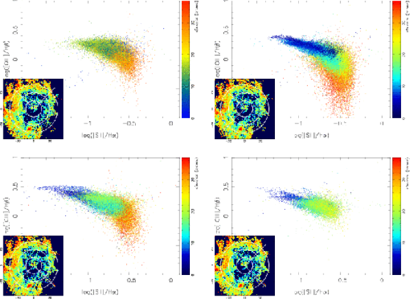
Figure 13: CIS pixel-by-pixel diagnostic diagram, log([O III] $\lambda$5007/H$\beta$) vs. log([S II] $\lambda$6717+6731H$\alpha$), for the four quadrants ($\pm 45\arcdeg$ centered on the four cardinal points, from left to right and from top to bottom, N, E, S, and W). The inset in each panel shows the [S II] $\lambda$6717+6731/H$\alpha$ image with superposed circles at radii of 10″, 20″, and 30″, and two lines indicating the quadrant plotted. The overall loci of the points in the diagram mark the general features of the CIS, and it is apparent that while the three diagrams corresponding to N$\pm 45\arcdeg$, E$\pm 45\arcdeg$, and S$\pm 45\arcdeg$ reach to very low values of log([O III] $\lambda$5007/H$\beta$) $<-0.5$ at large distances, the W$\pm 45\arcdeg$ diagram has all its pixels in the high to intermediate excitation regime, log([O III] $\lambda$5007/H$\beta$) $>-0.2$. This is strong evidence that the nebula is matter bounded towards the West.

We show in Fig. 12 maps of the three excitation ratios derived from the WFPC2 data, [O III] $\lambda$5007/H$\beta$, [S II] $\lambda$6717+6731/H$\alpha$, and [N II] $\lambda$6584/H$\alpha$. As we did for the H$\alpha$/H$\beta$ map, we first smoothed with a $5\times 5$ pixel box the continuum-subtracted emission-line images, calculated their ratios, and plotted the result with the low S/N ratio areas and bright stars masked out. Inspection of emission line diagnostic diagrams (Fig. 13) reveals two types of ionization structures: (a) a main central ionization structure (CIS) produced by the central SOBA, and (b) a number of secondary ionized structures (SISs) localized outside the main shell and energized by nearby small stellar groups.

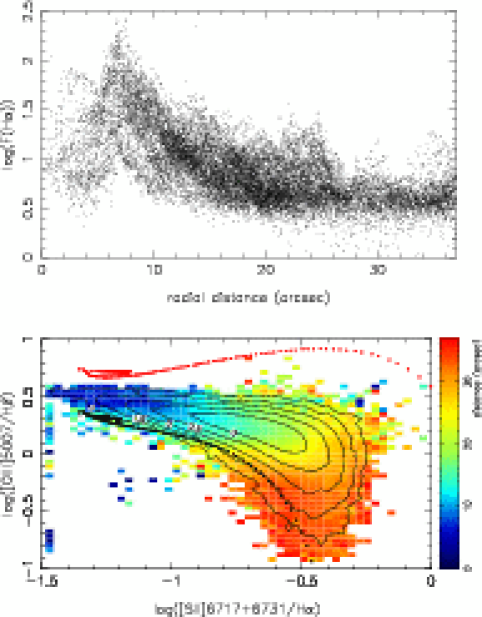
Figure 14: The top panel shows the radial distribution of the CIS H$\alpha$ flux (in log scale). The general appearance is that of an empty shell integrated along the line of sight, with an inner radius of 8″, given by the peak flux, plus an extended low surface brightness halo. The lower panel shows the log([O III] $\lambda$5007/H$\beta$) vs. log([S II] $\lambda$6717+6731/H$\alpha$) diagnostic diagram of the CIS. This diagram has been constructed from the pixel-by-pixel diagnostic diagram of the points belonging to the CIS, excluding those regions belonging to SISs. Each square represents the density of individual points located in that part of the diagram. The contours give the density of points in log scale (i.e., the contour labeled 3 indicates that that part of the diagram is populated by 1000 individual image pixels). The color codes for the average radial distance of those points to the CIS center. Two photoionization models (calculated using Cloudy) similar to those described in the simple approach followed by González Delgado & Pérez (2000) are plotted, the black points for an age of 2.75 Myr, and the red ones for an age of 3 Myr. The density distribution used is taken as the azimuthal average rms density distribution as obtained from the H$\alpha$ flux, and converted to actual density via the filling factor $\phi$ (taken as a parameter, and equal to 0.1 in the plot).

The CIS is dominated by the main shell (shell A) centered at (90″,9″). The upper panel in Fig. 14 shows the radial distribution of the CIS H$\alpha$ flux (in log scale), where it can be seen that the general appearance is that of an empty shell integrated along the line of sight, with an inner radius of 8″, plus an extended low-surface-brightness halo. The overall appearance of the CIS is that of an inner $\approx 20\arcsec$ radius high excitation zone surrounded by an outer larger low excitation halo. The high excitation zone is relatively symmetrical about the main shell. The low excitation halo is asymmetrical; it extends out to $\approx 45\arcsec$ towards the North, East and South, but it is significantly less important towards the West. Figure 13 shows the diagnostic diagram for four quadrants and a difference is readily apparent there in one of the four cardinal directions: the W$\pm 45\arcdeg$ diagram has all its pixels in the high to intermediate excitation regime, $\log(\mbox{[{O~{}III}]~{}$\lambda$5007}/\mbox{H$\beta$})>-0.2$, indicating that the nebula is density bounded towards the West.

The lower panel in Fig. 14 shows the log([O III] $\lambda$5007/H$\beta$) vs. log([S II] $\lambda$6717+6731/H$\alpha$) diagnostic diagram of the CIS. This diagram has been constructed from the pixel-by-pixel diagnostic diagram of the points belonging to the CIS, and where each square represents the density of individual points located in that part of the diagram. The contours give the density of points in log scale, while color is used to code the average radial distance of those points to the CIS center. We see that those points closer to the center (blue colors) have high excitation, while those further away (red) tend to be of lower excitation. Thus, this diagnostic diagram traces the overall ionization structure of the CIS, as expected for a simple shell+halo structure. We have run a series of models similar to those described in the simple approach followed by González Delgado & Pérez (2000). The density distribution used is taken as the azimuthal average rms density distribution as obtained from the H$\alpha$ flux, and converted to actual density via the filling factor $\phi$ (taken as a parameter). For a range of ages between 1 and 5 Myr, and $\phi=0.1,0.01,0.001$, we have used Cloudy (Ferland, 1997) with the same input SEDs as in González Delgado & Pérez (2000). The output radial distribution of emission line fluxes are integrated along the line of sight, assuming spherical symmetry. Only those models in the age range 2.75$-$3.0 Myr and $\phi=0.1$ fall close enough to the CIS ionization structure (see Fig. 14). We notice that: (i) as concluded by González Delgado & Pérez (2000), the age of the cluster ionizing the CIS is 2.5$-$3 Myr; and (ii) simple spherically symmetric models produce a well defined line in the diagnostic diagram, while the CIS points in NGC 604 are distributed along a thick region in the ionization structure. This spread in NGC 604 is produced by inhomogeneities in the detailed structure, with each radial direction from the center having a different actual density distribution. An additional cause for the spread is the fact that the ionizing stars are not all located at the center of the CIS, i.e., NGC 604 is ionized by a SOBA and not by a SSC.

Outside the main shell a number of SISs can be identified by their clear footprints on the diagnostic diagrams; they are ionized by a few or even just a single massive star. They are as follows.

• The filled H II region in region F, centered at (76″,5″) with a radius of 6″. The ionizing source consists of a small group that produces a maximum $\log(\mbox{[{O~{}III}]~{}$\lambda$5007}/\mbox{H$\beta$})=0.4$. The extinction is low, with $\mbox{$\tau_{\rm rad}$}=0.45$.

• The region around WR7, located at (104″,18″) with a radius of 1$\farcs$5. It is ionized by a single WR/Of star, identified as WR7 by Drissen et al. (1993), and reaches a high excitation value of $\log(\mbox{[{O~{}III}]~{}$\lambda$5007}/\mbox{H$\beta$})=0.6$. This star is located in a ridge where $\tau_{\rm Bal}$ grows rapidly from 0.7 to 1.2. As mentioned in the previous subsection, it also corresponds to a region of high density as measured from the [S II] $\lambda$6717/[S II] $\lambda$6731 ratio, possibly a compact H II region. If the star and the compact H II region are physically associated, the star should be an Of rather than a Wolf-Rayet.

• The filled H II region in region A, centered at (100″,17″) and with a radius of 2$\farcs$5, is the brightest and more compact within NGC 604. Ionized by a handful of UV-bright stars, it presents the highest ionization level, with up to $\log(\mbox{[{O~{}III}]~{}$\lambda$5007}/\mbox{H$\beta$})=0.75$. Located at the edge of the main molecular cloud, it has a value of $\tau_{\rm rad}$ of 0.92.

• The high-intensity H II gas in region B is elongated along the SN direction and just south of the filled H II region in region A. It has an approximate size of $6\arcsec\times 9\arcsec$ and its ionization level is not very high, $\log(\mbox{[{O~{}III}]~{}$\lambda$5007}/\mbox{H$\beta$})=0.35-0.40$, except in an unresolved high excitation knot at (100″,26″) where it reaches 0.6.

• Region E corresponds to the SNR described by D’Odorico et al. (1980) and it is centered at (94″,35″) with a radius of 1$\farcs$5. Its ionization footprint is conspicuous only in the ratio [S II] $\lambda$6717+6731/H$\alpha$, with logarithmic values between $-0.2$ and 0.0, with all other points in NGC 604 having values smaller that $-0.5$ for the log of this ratio. The excitation ratio [O III] $\lambda$5007/H$\beta$ has rather low values (logarithm between $-0.3$ and 0.2) except for the SE part of the SNR, where an [O III] $\lambda$5007-bright knot raises the value to $\log(\mbox{[{O~{}III}]~{}$\lambda$5007}/\mbox{H$\beta$})=0.4-0.5$. Contamination from the SNR hampers the measurement of the extinction, but an analysis of the surroundings indicate a low value. It is interesting to point out that the effect of the SNR on the global emission-line ratios for NGC 604 is very small, as evidenced by comparing the last two lines in either Table 3 or Table 4. It would be impossible to detect its presence using spatially-unresolved optical data.

• Another high-excitation region is located at (77″,9″) and has a radius of 1$\farcs$5. Given the symmetry of the local ionization structure, this node is probably ionized by a single star with a hard ionizing spectrum. The star is 0$\farcs$5 towards the W of the star identified as 139 by Drissen et al. (1993). The ionization level is high, with $\log(\mbox{[{O~{}III}]~{}$\lambda$5007}/\mbox{H$\beta$})=0.7$. Extinction is intermediate.

The detailed ionization structure of an H II region is related to the issue of whether all the ionizing radiation produced by the massive stars is processed within the nebula or whether some of it escapes into the more general interstellar medium of the host. González Delgado & Pérez (2000) modeled the integrated spectral properties of NGC 604, including an analysis of both the stellar spectral energy distribution (SED) and the photoionization of the integrated nebular spectrum. They concluded that, within this integrated modeling, the SED of the stars was adequate to account for the gas ionization and extension, and that there was no leak of ionizing radiation. The data presented here shows two pieces of evidence that argue against that statement. First, the western quadrant of the nebula appears to be matter bounded, as seen in the ionization structure and diagnostic diagrams shown above. Notice that the second largest molecular cloud is located in this direction, which in principle might seem incompatible with the matter bound scheme. This apparent discrepancy can be resolved if we locate the molecular cloud “behind” (along the line of sight) and the ionized gas is “in front”, as indicated by the extinction analysis above, and assume that the ionized cloud is “broken” so that the radiation escapes after producing the O⁺⁺ zone and there is no ionization front trapped in this direction. Second, we have measured the velocity field along the 14″-wide WHT scan spectrum at PA=60$\arcdeg$. Figure 15 shows the velocity field of H$\beta$ (filled points) and of [O III] $\lambda$5007 (open circles), together with the H$\beta$ flux distribution (dotted line). The horizontal line marks the systemic velocity of $-255$ km s^-1 (Tenorio-Tagle et al., 2000) and the horizontal scale (in ″) is centered in the main shell (seen as the two rather asymmetrical peaks in the flux distribution), increasing towards the SW. At the SW edge of the shell the gas velocity suddenly jump to $-270$ km s^-1. This blue-shifted high-excitation ionized gas can be interpreted as further evidence that the shell has been broken and that the shreds have been blown out onto the line of sight, as suggested by Tenorio-Tagle et al. (2000). In any case, the final word on the nature of NGC 604 as an ionization- or matter-bounded nebula requires a complete characterization of the young stellar population, which we will address in a subsequent paper.

5 DISCUSSION AND CONCLUSIONS

A consistent picture emerges from our analysis of the gas distribution in NGC 604: the $\approx 3.0$ Myr-old MYC (González Delgado & Pérez, 2000; Maíz-Apellániz, 2000) has carved a hole in its surrounding ISM and HAS punctured it in several places, leading to the formation of a series of cavities and tunnels. This low-density medium is filled with hot coronal gas that emits in X-rays and is transparent to the ionizing UV radiation. The leftover molecular gas from the parent cloud is still visible along several directions, but for others, including the direct line of sight to the central part of the SOBA, it appears to have been almost completely cleared out. What we see as a giant H II region is a composite of (a) localized high-intensity, high-excitation gas on the surfaces of the molecular clouds directly exposed to the ionizing radiation, and (b) a diffuse low-intensity, low-excitation component that extends for several hundreds of pc. A similar morphology is also observed in 30 Doradus. Both objects have a similar partition of the fluxes for different emission lines, with most of the photons from medium and high excitation species (e.g. H$\alpha$ and [O III] $\lambda$5007) being produced in the surfaces adjacent to the molecular clouds and a more even distribution for the photons from low-excitation species (e.g. [S II] $\lambda$6717+6731 and [N II] $\lambda$6584). The high-excitation regions are indeed near-bidimensional in character, given that their thicknesses ($\sim 1$ pc) are much smaller than their extensions (several tens of pc), so that a more appropriate name for them may be H II surfaces. The morphology of the H II gas in the halo is less clear: does it fill most of the volume around the giant H II region or is it concentrated in a series of thin shells? The complex kinematics of the halo of both 30 Doradus (Chu & Kennicutt, 1994) and NGC 604 (Yang et al., 1996; Maíz-Apellániz, 2000), where two or more individual kinematic components are detected in most positions, favors the second option. This H II surface + extended halo morphology observed in NGC 604 and 30 Doradus (Walborn et al., 2002) is also consistent with what is observe in objects at larger distances and lower spatial resolutions, such as NGC 4214-II (MacKenty et al., 2000), where the low-excitation halo is easily resolved but the H II surface is reduced to a quasi-point-like high excitation core.

Assuming the validity of the comparison between the structure of the giant H II region in NGC 604 and in other objects such as 30 Doradus, we can make two predictions for future observations. One is that wherever H II surfaces are present one should also detect the PDR in e.g. the NIR H₂ emission lines (Rubio et al., 1998). The second one is that if we obtain higher-resolution images of the H II surfaces, we should detect dust pillars similar to the ones seen from the Eagle Nebula to 30 Doradus (Scowen et al., 1998; Walborn, 2002). Those pillars should be easier to detect where the H II surface is seen near-edge-on and should be locations where induced star formation may be taking place. Another such place where we may be witnessing induced star formation is the bright compact H II region in region A, which is similar to knot 1 in 30 Doradus in terms of apparent stellar content, orientation with respect to the molecular cloud, and high surface brightness (Walborn et al., 2002).

For distant giant H II regions we cannot resolve the individual components and we can only analyze their spatially-integrated properties. Our analysis suggests that characterization of the extinction from spatially-integrated studies might be quite uncertain, especially when the amount of dust is relatively large. Taking NGC 604 as an example, if we would perform an integrated study of its properties, the underestimation of the number of ionizing photons as derived from the $F_{\alpha}/F_{\beta}$ ratio would be around 27%, compared to an underestimation of around 11% derived from our high-spatial-resolution data. Just for comparison, if no correction at all is applied, the underestimation increases to around 42%. In principle, the analysis of the radio continuum could provide a good estimate of the ionizing flux being emitted, indeed more accurate than the value derived from the Balmer lines ratio. Nevertheless, we want to stress that the non-thermal contribution to the radio continuum could lead to an overestimation of the ionizing flux, unless high-resolution radio observations are used to separate the contributions from non-thermal emitting regions. In the case of relatively unevolved regions, like NGC 604, the non-thermal component is negligible ($\approx 1\%$ at 3.6 cm), but it might be significant for other objects (see MacKenty et al. 2000 for NGC 4214). We want to stress that the uncertainties in the ionizing flux values derived from emission lines or thermal radio continuum make it very uncertain to derive the number of ionizing photons escaping unabsorbed from the region, unless a careful analysis of both the stellar population and the structure of the absorbing agents is performed.

The reason why it is not possible to produce a simple correction for the attenuation experienced by the gas is the intrinsically complex geometry of a giant H II region. The sources (H II surfaces and halos) and the extinction agents (the dust particles located mainly in the adjacent molecular clouds) are extended and, to a certain degree, intermixed. As a consequence, sources located in different points in the plane of the sky may have quite different amounts of dust in front of them. Furthermore, two sources along the same line of sight may have large amounts of dust between them, as we have seen for the case of the “flaps”. Our WFPC2 images show how extinction can rapidly vary in scales of a pc or less and that even relatively small structures of the order of a few tens of pc can hide a significant fraction of the optically-unobservable H II gas. We estimate that most of the $\lesssim 11\%$ of the H$\alpha$ flux that is not recoverable except using radio (or maybe NIR) observations could be accounted for simply by extending the optically bright H II surfaces in the B and CD regions into an area equivalent to the one covered by each flap, as derived from the optical geometry in Fig. 3 (10-20 square arcseconds in each case).

This complex geometry of GHRs explains the well known effect that in many galaxies hosting strong starbursts the average extinction experienced by the stars is significantly lower than the integrated extinction derived from the Balmer emission lines, as discussed e.g. by Calzetti et al. (2000). In NGC 604 the SOBA is located in a low extinction region because it has cleared out a cavity around it. A similar result was obtained for NGC 4214 (Maíz-Apellániz et al., 1998). In the next paper we will analyze the extinction affecting the stellar continuum of the individual stars in NGC 604 one by one, in more detail.

We can conclude that in NGC 604 a large fraction of the extinction is caused by dust associated with the GHR itself, although not evenly distributed. A similar conclusion was reached by Caplan & Deharveng (1986) for H II regions in the LMC using unresolved data. It should be pointed out that those authors indicated already almost twenty years ago that one of the ways to continue work in this field was by using “point-by-point emission-line photometry”. Our analysis shows that this technique allows indeed a better characterization of the extinction properties and, moreover, confirms the results obtained by these authors on the LMC GHRs.

The main cavity in NGC 604 has a diameter of $\approx 60$ pc, which is several times smaller than the value predicted by applying the single-star wind-blown model of Weaver et al. (1977). According to that model, bubble sizes should be very weakly dependent on wind luminosity or on the density of the surrounding medium, so varying those parameters does not provide a solution to the discrepancy. As a matter of fact, any of the four cavities in NGC 604 could have been created by the kinetic energy released into their surroundings by only one or a few massive stars (as opposed to the $\approx 200$ here) in a period of 3 Myr if Weaver et al. (1977) models were applicable here. This discrepancy is similar to the ones found for NGC 4214 and other objects by MacKenty et al. (2000) and Maíz-Apellániz (2001). We believe that the explanation lies in that the ISM is far from being in pressure equilibrium. Recent numerical simulations by Mac Low (2004) show that the ISM is extremely dynamic, with molecular clouds being transient objects formed along the edges of superbubbles by the collision of two or more of them. In those simulations, the gas compressed in such a way can collapse to form stellar clusters but may have only a short time to do so, since superbubbles come and go in scales of only $\sim 10$ Myr. In other environments, such as dwarf galaxies, MYCs may form in a different way but the requirement for a source of external pressure should still be present. NGC 604 is known to be located at the edge of an H I-detected superbubble centered $\sim 1$ kpc towards the SE (Thilker, 2000). According to the previously mentioned simulations, that superbubble may have triggered the formation of NGC 604 and should still be pushing the two largest molecular clouds associated with NGC 604 in the opposite direction to the one in which the winds and SNe from the NGC 604 SOBA are pushing them (see Fig. 3 in Thilker 2000). That source of external pressure is likely to be one of the reasons for the smaller-than-expected sizes of the bubbles in NGC 604.

Two additional mechanisms that act to make superbubbles smaller than their expected sizes at a given age may also be in effect. On the one hand, when a giant molecular cloud is formed and once the gas becomes dense enough, its pressure should increase locally due to self-gravity. Under those conditions, wind bubbles from isolated stars have to fight an additional pressure and have difficulty expanding to their expected sizes, especially in the first stages of their development (García-Segura & Franco, 1996). In a stationary isolated case, the growth of a wind-blown bubble can stall completely. In a more realistic environment, the motion of the star should eventually take it out of its dense birth region and its bubble may expand to a size large enough to find an adjacent bubble. The resulting wind-wind collision should lead to a second thermalization (the first one being produced by the initial reverse shock wave created by the interaction of the stellar wind with its surrounding dense medium) and, after adding more recently-formed massive stars to the bubble, become the seed for a superbubble. However, the whole process may be delayed by several hundreds of thousands of years by the initial confinement of the individual bubbles, thus contributing to the excess in the number of giant H II regions without superbubbles detected by Maíz-Apellániz (2001). The second mechanism that should contribute to the small observed sizes of superbubbles lies in the inhomogeneity of the large-scale ISM. Once a superbubble expands to a size of $\sim 100$ pc, it is likely to encounter a density gradient in one or several directions. The superbubble is then punctured and the hot coronal gas flows out of the cavity through the created hole(s). The subsequent reduction in the internal pressure of the cavity should slow down its expansion and, eventually, halt it and even reverse it. As discussed by Tenorio-Tagle et al. (2000), the observed morphology and kinematics of NGC 604 is consistent with such a puncture.

In this paper we have presented our results on the spatial distribution of the different gas phases and the dust in NGC 604. In the next paper we will study the massive stellar population by means of HST UV-optical photometry and HST UV objective-prism spectroscopy. The analysis of the individual stars will provide a complete picture of the relationship between the gas and the stars in NGC 604, and will allow to measure the fraction of ionizing photons that potentially escape from the nebula into the general ISM of M33.

APPENDIX: DUST MODELS

The ratio between the H$\alpha$ and radio emissivities of a photoionized region with $n({\rm He}^{+})/n({\rm H}^{+})=0.09$ for case B is (Caplan & Deharveng, 1986; Churchwell & Goss, 1999):

$$q\frac{j_{\alpha}\mbox{ (erg s\mbox{${}^{-1}$}\ cm\mbox{${}^{-2}$})}}{j_{\nu}\mbox{ (Jy)}}=\mbox{$7.90\cdot 10^{-10}$}\left(\frac{T}{10^{4}\mbox{ K}}\right)^{-0.59}\left(\frac{\nu}{10^{9}\mbox{ Hz}}\right)^{0.1},$$ (1)

where the possible errors due to the power-law approximations used and the possible uncertainty in the He abundance are of the order of a few percent. From Eq. 1 we obtain that the (true) optical depth at H$\alpha$ measured from the radio and H$\alpha$ fluxes, $F_{\nu}$ and $F_{\alpha}$:

$$\mbox{$\tau_{\rm rad}$}=\ln\left[\mbox{$1.27\cdot 10^{9}$}\left(\frac{T_{e}}{10^{4}\mbox{ K}}\right)^{0.59}\left(\frac{\nu}{10^{9}\mbox{ Hz}}\right)^{-0.1}\frac{F_{\nu}(\mbox{Jy})}{F_{\alpha}(\mbox{erg s}^{-1}\mbox{ cm}^{-2})}\right],$$ (2)

For NGC 604, we use T = 8 500 K (Díaz et al., 1987; González Delgado & Pérez, 2000; Esteban et al., 2002) and for the frequency of $\nu$ = 8.44 GHz of Churchwell & Goss (1999) Eq. 2 becomes:

$$\mbox{$\tau_{\rm rad}$}=\ln\left[\mbox{$9.32\cdot 10^{8}$}\frac{F_{\nu}(\mbox{Jy})}{F_{\alpha}(\mbox{erg s}^{-1}\mbox{ cm}^{-2})}\right],$$ (3)

The corresponding ratio between the H$\alpha$ and H$\beta$ emissivities is, within $\sim$ 1%:

$$\frac{j_{\alpha}}{j_{\beta}}=2.859\left(\frac{T}{10^{4}\mbox{ K}}\right)^{-0.07},$$ (4)

where the two emissivities are measured in the same units. From Eq. 4 and the Cardelli et al. (1989) law for $R_{V}=3.2$ we obtain the optical depth at H$\alpha$ measured from the ratio of the two Balmer fluxes, $F_{\alpha}$ and $F_{\beta}$:

$$\mbox{$\tau_{\rm Bal}$}=2.42\ln\left[\frac{F_{\alpha}/F_{\beta}}{2.859}\left(\frac{T_{e}}{10^{4}\mbox{ K}}\right)^{0.07}\right],$$ (5)

which for T = 8 500 K becomes:

$$\mbox{$\tau_{\rm Bal}$}=2.42\ln\left[\frac{F_{\alpha}/F_{\beta}}{2.892}\right].$$ (6)

One of the largest uncertainties in measuring $\tau_{\rm Bal}$ comes from the assumed value of $R_{V}$. For example, values of 2.6 or 4.4 change the constant that multiplies the logarithm in Eq. 5 to 2.04 and 3.07, respectively. Here we will ignore this question but we plan to study it in future works.

The standard attenuation model is that of a uniform foreground screen model. There we have that $\tau_{\rm rad}$=$\tau_{\rm Bal}$, since all areas observed are affected by dust in the same degree and no scattering is injecting photons back into the line of sight.

A uniform foreground screen is not very realistic for H II regions, since images reveal the existence of localized dust clouds. Here we explore a model in which we assume that the dust in the aperture is distributed in a patchy foreground screen, in such a way that the area covered is $\gamma$ times the area free of dust and the screen yields an optical depth at H$\alpha$ of $\tau_{\rm cov}$ for the areas behind it. In this case, the values of $\tau_{\rm rad}$ and $\tau_{\rm Bal}$ for the aperture will be weighted means of $\tau_{\rm cov}$ (the optical depth experienced by the areas covered by dust) and zero (the optical depth experienced by the areas free of dust).

Our results are shown in Fig. 8, where we represent $\tau_{\rm Bal}$ as a function of $\tau_{\rm rad}$ for different values of $\gamma$. As expected, $\tau_{\rm Bal}$ is always smaller than $\tau_{\rm rad}$ when the dust is not in a uniform foreground screen and scattering is not relevant (see e.g. Caplan & Deharveng 1986. For our patchy foreground screen model, $\tau_{\rm Bal}$ first increases while the obscured areas contribute significantly to the detected radiation. When the amount of dust present in the screen becomes large enough, the curve acquires a negative slope and ends up going back to zero since the dominant effect is to let only the unobscured regions contribute to the detected Balmer photons. Note that the region defined by $\mbox{$\tau_{\rm Bal}$}\geq 0$, $\mbox{$\tau_{\rm rad}$}\geq\mbox{$\tau_{\rm Bal}$}$ is completely covered by the family of models for $\mbox{$\tau_{\rm cov}$}\geq 0$, $0\leq\gamma\leq 1$, with a one-to-one mapping which is only degenerate for $\mbox{$\tau_{\rm Bal}$}=\mbox{$\tau_{\rm rad}$}=0$.

Figure 8: $\tau_{\rm Bal}$ vs. $\tau_{\rm rad}$ for a patchy foreground model with different values of $\gamma$, the area covered by the screen. Dashed lines show the location of different values of the optical depth of the screen. The values obtained for our regions are also plotted.

 

Figure 10: (left) H$\alpha$ flux and electron density at $y=17\farcs 3$ derived from slit data as a function of the horizontal coordinate established in Fig. 9. The density has been smoothed with a 3-pixel (1″) box. H$\alpha$ is expressed in units of $20\cdot 10^{-17}$ erg s^-1 cm^-2 arcsec^-2 and $n_{e}$ is expressed in cm^-3. (right) True optical depth at H$\alpha$, CO ($1\rightarrow 0$) intensity, and electron density at $x=105\farcs 3$ as a function of the vertical coordinate established in Fig. 9. $\tau_{\rm rad}$ is obtained from Churchwell & Goss (1999), the CO data is from Engargiola et al. (2003), and $n_{e}$ is derived from slit data. The density has been smoothed with a 9-pixel (3″) box. The value of $\tau_{\rm rad}$ can be read directly from the labels in the vertical axis, the CO scale is arbitrary, and $n_{e}$ is expressed in units of 300 cm^-3.

 

Figure 11: H$\alpha$ flux, $\tau_{\rm Bal}$, and [O III] $\lambda$5007/H$\beta$ measured from WFPC2 data as a function of the horizontal coordinate established in Fig. 9. The left figure corresponds to $y=16\farcs 6$ and the right one to $y=13\farcs 4$. H$\alpha$ is shown in arbitrary units while the scale for $\tau_{\rm Bal}$ and [O III] $\lambda$5007/H$\beta$ can be read from the left and right sides, respectively.

Figure 15: Velocity field of H$\beta$ (filled points) and of [O III] $\lambda$5007 (open circles), together with the H$\beta$ flux distribution (dotted line). The horizontal line marks the systemic velocity of $-255$ km s^-1 (Tenorio-Tagle et al., 2000). The abcissa scale is centered in the main shell (seen as the two rather asymmetrical peaks in the flux distribution) and increases towards the SW. At the SW edge of the shell the gas velocity suddenly jump to $-270$ km s^-1. This blue-shifted high-excitation ionized gas can be interpreted as further evidence that the shell has been broken and that the shreds have been blown out onto the line of sight, as suggested by Tenorio-Tagle et al. (2000).

References

- Anderson & King (2003) Anderson, J., & King, I. R. 2003, PASP, 115, 113
- Barbá et al. (2003) Barbá, R. H., Rubio, M., Roth, M. R., & García, J. 2003, AJ, 125, 1940
- Bluhm et al. (2003) Bluhm, H., de Boer, K. S., Marggraf, O., Richter, P., & Wakker, B. P. 2003, A&A, 398, 983
- Bosch et al. (2002) Bosch, G., Terlevich, E., & Terlevich, R. 2002, MNRAS, 329, 481
- Calzetti et al. (2000) Calzetti, D., Armus, L., Bohlin, R. C., Kinney, A. L., Koornneef, J., & Storchi-Bergmann, T. 2000, ApJ, 533, 682
- Calzetti et al. (2004) Calzetti, D., Harris, J., Gallagher, J. S., III, Smith, D. A., Conselice, C. J., Homeier, N., & Kewley, L. 2004, AJ, 127, 105
- Caplan & Deharveng (1986) Caplan, J., & Deharveng, L. 1986, A&A, 155, 297
- Cardelli et al. (1989) Cardelli, J. A., Clayton, G. C., & Mathis, J. S. 1989, ApJ, 345, 245
- Casertano & Wiggs (2001) Casertano, S., & Wiggs, M. S. 2001, WFPC2 Instrument Science Report 2001-10 (STScI)
- Castañeda et al. (1992) Castañeda, H. O., Vílchez, J. M., & Copetti, M. V. F. 1992, A&A, 260, 370
- Cerviño et al. (2002) Cerviño, M., Mas-Hesse, J. M., & Kunth, D. 2002, A&A, 392, 19
- Chu & Kennicutt (1994) Chu, Y.-H., & Kennicutt, R. C., Jr. 1994, ApJ, 425, 720
- Churchwell & Goss (1999) Churchwell, E., & Goss, W. M. 1999, ApJ, 514, 188
- Díaz et al. (1987) Díaz, A. I., Terlevich, E., Pagel, B. E. J., Vílchez, J. M., & Edmunds, M. G. 1987, MNRAS, 226, 19
- D’Odorico et al. (1980) D’Odorico, S., Dopita, M. A., & Benvenuti, P. 1980, A&AS, 40, 67
- Dolphin (2000) Dolphin, A. E. 2000, PASP, 112, 1383
- Drissen et al. (1993) Drissen, L., Moffat, A. F. J., & Shara, M. M. 1993, AJ, 105, 1400
- Engargiola et al. (2003) Engargiola, G., Plambeck, R. L., Rosolowsky, E., & Blitz, L. 2003, ApJS, 149, 343
- Esteban et al. (2002) Esteban, C., Peimbert, M., Torres-Peimbert, S., & Rodríguez, M. 2002, ApJ, 581, 241
- Fall & Rees (1977) Fall, S. M., & Rees, M. J. 1977, MNRAS, 181, 37P
- Ferland (1997) Ferland, G. J. 1997, Hazy, a brief introduction to Cloudy (University of Kentucky, Department of Physics and Astronomy Internal Report)
- Ferland (2001) Ferland, G. J. 2001, PASP, 113, 41
- Freedman et al. (2001) Freedman, W. L., et al. 2001, ApJ, 553, 47
- García-Segura & Franco (1996) García-Segura, G., & Franco, J. 1996, ApJ, 469, 171
- González Delgado & Pérez (2000) González Delgado, R. M., & Pérez, E. 2000, MNRAS, 317, 64
- Gordon et al. (1998) Gordon, S. M., Kirshner, R. P., Long, K. S., Blair, W. P., Duric, N., & Smith, R. C. 1998, ApJS, 117, 89
- Hollenbach & Tielens (1997) Hollenbach, D. J., & Tielens, A. G. G. M. 1997, ARA&A, 35, 179
- Hunter et al. (1996) Hunter, D. A., Baum, W. A., O’Neil, E. J., Jr., & Lynds, R. 1996, ApJ, 456, 174
- Kozhurina-Platais et al. (2003) Kozhurina-Platais, V., Anderson, J., & Koekemoer, A. M. 2003, WFPC2 Instrument Science Report 2003-02 (STScI)
- Mac Low (2004) Mac Low, M.-M. 2004, in How does the Galaxy work? A Galactic tertulia with Don Cox and Ron Reynolds, E. Alfaro, E. Pérez, and J. Franco (eds.), (Dordrecht: Kluwer Academic Publishers), in press
- MacKenty et al. (2000) MacKenty, J. W., Maíz-Apellániz, J., Pickens, C. E., Norman, C. A., & Walborn, N. R. 2000, AJ, 120, 3007
- Maíz-Apellániz (2001) Maíz-Apellániz, J. 2001, in Highlights of Spanish astrophysics II, J. Zamorano, J. Gorgas, and J. Gallego (eds.), Fourth Scientific Meeting of the Spanish Astronomical Society (Dordrecht: Kluwer), 113
- Maíz-Apellániz (2000) Maíz-Apellániz, J. 2000, PASP, 112, 1138
- Maíz-Apellániz (2001) Maíz-Apellániz, J. 2001, ApJ, 563, 151
- Maíz-Apellániz et al. (1998) Maíz-Apellániz, J., Mas-Hesse, J. M., Muñoz-Tuñón, C., Vílchez, J. M., & Castañeda, H. O. 1998, A&A, 329, 409
- Ochsenbein et al. (2000) Ochsenbein, F., Bauer, P., & Marcout, J. 2000, A&AS, 143, 221
- O’Dell (2001) O’Dell, C. R. 2001, ARA&A, 39, 99
- O’Dell & Doi (1999) O’Dell, C. R., & Doi, T. 1999, PASP, 111, 1316
- Parker et al. (1992) Parker, J. W., Garmany, C. D., Massey, P., & Walborn, N. R. 1992, AJ, 103, 1205
- Rubin et al. (2002) Rubin, R. H., et al. 2002, MNRAS, 334, 777
- Rubio et al. (1998) Rubio, M., Garay, G., & Probst, R. 1998, The Messenger, 93, 38
- Russell et al. (1990) Russell, J. L., Lasker, B. M., McLean, B. J., Sturch, C. R., & Jenkner, H. 1990, AJ, 99, 2059
- Sabalisck et al. (1995) Sabalisck, N. S. P., Tenorio-Tagle, G., Castañeda, H. O., & Muñoz-Tuñón, C. 1995, ApJ, 444, 200
- Scowen et al. (1998) Scowen, P. A., et al. 1998, AJ, 116, 163
- STScI (1999) STScI. 1999, Synphot User’s Guide, Howard Bushouse and Bernie Simon (eds.)
- STScI (2002) STScI. 2002, WFPC2 Data Handbook, Sylvia Bagget and Matthew Mc Master (eds.)
- Tenorio-Tagle et al. (1996) Tenorio-Tagle, G., Muñoz-Tuñón, C., & Cid-Fernandes, R. 1996, ApJ, 456, 264