Experimental Study of Acoustic Ultra-High-Energy Neutrino Detection

Abstract

An existing array of underwater, large-bandwidth acoustic sensors has been used to study the detection of ultra-high-energy neutrinos in cosmic rays. Acoustic data from a subset of 7 hydrophones located at a depth of $\sim 1600$ m have been acquired for a total live time of 195 days. For the first time, a large sample of acoustic background events has been studied for the purpose of extracting signals from super-EeV showers. As a test of the technique, an upper limit for the flux of ultra-high-energy neutrinos is presented along with considerations relevant to the design of an acoustic array optimized for neutrino detection.

I Introduction

The detection of a neutrino component in cosmic rays above $10^{19}$ eV is a central goal of particle astro-physics. It is generally believed (Greisen, 1966; Zatsepin & Kuzmin, 1966) that the flux of cosmic ray protons should drop sharply (“GZK” cutoff) between $10^{19}$ and $10^{20}$ eV due to pion photo-production on the microwave background. Recent measurements using the AGASA surface array (Takeda et al., 1999) and the HiRes air fluorescence telescope (Abbasi et al., 2002) seem to disagree on the existence of such a cutoff, although it has been pointed out (Bahcall & Waxman, 2003) that they may actually be consistent with one another. Neutrinos are likely to be an important component of the particle flux at ultra-high energies. If the GZK mechanism is indeed present, the flux of ultra-high energy protons must be accompanied by ultra-high energy neutrinos (“GZK” neutrinos) from pion decay. Their clear detection would provide crucial input to the field.

Detection of the very small flux of cosmic rays at these extreme energies requires detectors of unprecedented size. Therefore only detectors employing naturally occurring media are practical. The parallel development of several different techniques, some of which would ideally employ the same medium, is therefore crucial to constraining the measurements and providing sufficiently accurate and redundant information in order to fully understand cosmic rays at the highest energies. Indeed, in the last few years, great progress has been made in the use of radio signals for the detection of protons and neutrinos using a variety of natural targets, including lunar regolith (Gorham et al., 2003) and ice with ground- (Kravchenko et al., 2003) and space-based (Lehtinen et al., 2004) antennas.

In this paper we describe the first experimental results obtained with the acoustic technique in ocean water. The possibility of acoustic detection of high-energy particles was first discussed in 1957 (Askaryan, 1957; Askaryan & Dolgoshein, 1977). Following this work, an extensive theoretical analysis of the processes relevant to signal formation was performed (Learned, 1979), and the general phenomenon was confirmed with an accelerator test beam (Sulak et al., 1979). The first description of the properties of a practical, large array for ultra-high-energy neutrino detection was given in (Lehtinen et al., 2002). The dominant sound production mechanism, for non-zero water expansivity, consists of water heating in the region where a shower develops (instantaneously, from the point of view of acoustics), followed by expansion, producing a pressure wave. Only primaries that penetrate the atmosphere without interacting and then shower in the water are capable of producing detectable acoustic pulses, providing automatic particle identification within a broad range of energies. Acoustic sensor arrays can be substantially more sparse than optical Cherenkov arrays in water or ice, because of the large ($\approx 1$ km) attenuation length of sound in water at the frequencies ($\approx 10$ kHz) where, for these events, most of the energy lies. However, as stressed in (Lehtinen et al., 2002), the elongated shape of the showers produces acoustic interference that results in most of the sound emitted in a pancake-shaped volume with few degrees opening angle. This effect is important for the optimization of a detector since the optimal density of hydrophones is constrained by the ability to intercept these relatively narrow pancakes. Finally the acoustic technique lends itself well to a calorimetric measurement of the total energy and would complement other technologies well.

II The Detector

SAUND (Study of Acoustic Ultra-high energy Neutrino Detection) employs a large ($\sim 250$ km²) hydrophone array in the U.S. Navy Atlantic Undersea Test And Evaluation Center (AUTEC). The array is located in the Tongue of the Ocean, a deep tract of sea in the Bahama islands at approximately $24^{\circ}30^{\prime}N$ and $77^{\circ}40^{\prime}W$. A detailed description of the entire array is given in (Lehtinen et al., 2002). For the present work, we use a subset of seven hydrophones from the large array, arranged in a hexagonal pattern as shown in Figure 1. The hydrophones are mounted on 4.5 m booms standing vertically on the ocean floor. The horizontal spacing between central and peripheral hydrophones is between 1.50 km and 1.57 km. The ocean floor is fairly flat over the entire array region, with our phones located at depths between 1570 m and 1600 m. The hydrophones and their underwater preamplifiers have been in stable operation for naval exercises since 1969.

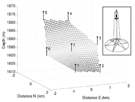
Figure 1: Schematic view of the subset of hydrophones used for this work. The hydrophone depths are known precisely while the sea floor bathymetry between phones is estimated with a linear interpolation. The inset shows the 4.5 m tall hydrophone deployment and support structure. The bail used to deploy the phone folds and lies on the ocean floor during operation.

Analog signals are amplified at the hydrophones and fed through an on-shore amplifier stage to a digitizer card that continuously samples each of the seven channels at 179 ksamples/s. The time series in each channel is then fed to a digital matched filter implemented on a 1.7 MHz Pentium-4 workstation.

Ultra-high energy neutrinos interact with matter by deep inelastic scattering on quarks inside nuclei. With increasing energy, the interaction cross-section (Kwi et al, 1999), and hence the probability of a neutrino interacting within the ocean water (which is thinner than the $\sim 100$ km interaction length at 10²¹ eV), increases. After the primary interaction, the neutrino energy is distributed between a quark and a lepton. On average, the lepton acquires $\sim$80% of the energy (Gandhi et al, 1996). The remaining energy is dumped into the water as a hadronic shower aligned with the direction of the primary neutrino. The water is heated locally, causing it to expand and emit an acoustic pulse propagating perpendicular to the shower axis.

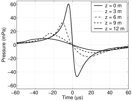
Figure 2: Simulated acoustic signals due to a hadronic shower of energy $10^{20}$ eV, corresponding to an initial neutrino energy of $5\times 10^{20}$ eV. Signals are shown at 1050 m distance perpendicular to the neutrino path. The five different curves refer to longitudinal distances of 0, 3, 6, 9, and 12 m forward from the shower maximum.

While a muon or tau neutrino generates only a hadronic shower, an electron neutrino also generates an electromagnetic shower, which is superimposed on the hadronic one. However, due to the Landau-Pomeranchuk-Migdal (LPM) effect (Landau & Pomeranchuk, 1935; Migdal, 1956, 1957), the electromagnetic shower is elongated and has an irregular structure, producing weaker acoustic signals with irregular geometries. Here we only consider the hadronic showers, which exhibit the same structure for all kinds of neutrinos and are simulated with a simple parametrization as modeled in (Alvarez & Zas, 1998). This model includes $\pi_{0}$ interactions and the LPM effect for the electromagnetic components of the hadronic shower. Once the energy deposition has been determined using this shower model, the resulting acoustic pulse shape is simulated, following (Learned, 1979; Lehtinen et al., 2002), at arbitrary positions ($r,\theta$) with respect to the shower. As shown in Figure 2 for a fixed radial distance from the shower, the bipolar pulse is tallest and narrowest in a plane perpendicular to the shower axis, at the longitudinal location of the shower maximum. The pulse becomes shorter and wider at greater longitudinal distances from the maximum. The general features of the pulse shape match the data from (Sulak et al., 1979).

Triggering is achieved in SAUND with a digital matched filter that searches for signals matching the expected neutrino signal, appropriately weighting frequency components according to their signal-to-noise ratio (Hogg & Craig, 1995). The filter response function is obtained by transforming to the frequency domain the expected signal shape, which is approximated in the time domain by the analytical form $S(t)\propto-(t/\tau)e^{-t^{2}/{2\tau^{2}}}$. The characteristic time of the signal depends on position $(r,\theta)$ relative to the shower (see Figure 2). A characteristic time of $\tau=10$ $\mu$s, corresponding to the width of the largest expected signals, is chosen for the present work. To obtain the filter transfer function, the expected signal in the frequency domain, $\tilde{S}(f)$, is divided by the noise spectrum, assumed to be of the Knudsen type (Knudsen et al., 1948): $\tilde{N}(f)\propto f^{-\alpha}$. The expected $\alpha=1.7$ is approximated with $\alpha=2$ for analytical convenience. The transfer function $\tilde{H}\propto\tilde{S}(f)/\tilde{N}(f)$ is then transformed to the time domain to obtain the response function,

$$H(t)=\left[\left(\frac{t}{\tau}\right)^{3}-3\left(\frac{t}{\tau}\right)\right]e^{-t^{2}/{2\tau^{2}}}.$$ (1)

Each channel is continuously filtered and the filter output is compared to a threshold. The filter is implemented with a discretized version of the above response function, sampled at the same frequency as the pressure waveforms (179 kHz). 12 samples ranging from $t=-30.8~{}\mu$s to $t=30.8~{}\mu$s are used. Beyond this range, the response function is below 13% of its peak amplitude. When the threshold is exceeded, a trigger occurs and event data are recorded.

Signals from the highest-energy neutrinos considered here are expected to saturate the digitizer, and $\sim 10\%$ of waveforms in the dataset are saturated. By simulating the effects of saturation on the digital filter and on subsequent offline cuts, we found that saturation does not pose a problem to the present analysis. This is because the cuts rely primarily on frequency and timing information, not on amplitude.

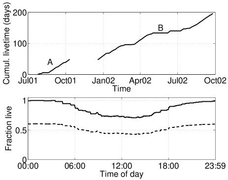
Figure 3: Live time for SAUND. In the top panel, we show the data accumulation as a function of time. A test run (Run A, 48 days), not used in the present analysis, was followed by a system upgrade and a longer period of stable running (Run B, 147 days). In the bottom panel, the solid curve gives the fraction live as a function of time of day, for days during which any SAUND Run B data were collected. The dashed curve represents the data used for the analysis reported here, and it includes down time from bad weather and hardware failures.

By arrangement with the U.S. Navy, the SAUND data acquisition system (DAQ) is connected to the hydrophone array only when the array is not in use for Navy exercises. The live time achieved under this agreement is shown in Figure 3. As shown in the top panel, a test run (Run A) was used to commission the system and is not used for the present analysis. The system was upgraded from Oct. 2001 to Dec. 2001 and run for an integrated 147 days live with stable conditions (Run B). Only this stable run is used for the analysis presented here. The solid curve in the bottom panel shows the live time achieved at different times of day. The live time is close to 100% at night, when no Navy tests are conducted, and it drops to about 70% in the middle of the day. The average over a day is $86\%$. In addition, an overall live time reduction due to weather conditions and hardware failures resulted in the dashed line in the bottom panel of Figure 3.

Because the noise environment is volatile, an adaptive trigger threshold is used. Every minute the threshold is raised or lowered based on whether the number of events in the previous minute was above or below the target rate of 60 events/minute. Events are accumulated in memory each minute and written to disk, along with data relevant to the entire minute, at the end of the minute. The distribution of thresholds in Run B is shown in Figure 4. To simplify online processing and offline event reconstruction, the threshold value is constrained to discrete values (integer multiples of 0.004, in units of digital filter output). For the purpose of neutrino analysis, only thresholds between 0.012 and 0.024 are used. These “quiet” periods account for 37% of Run B.

In total, Run B contains 20 M triggers (250 GB) corresponding to $\sim$1.7 GB/day. Every few weeks, data are transferred to an external hard drive that is shipped to Stanford for offline analysis. Nine-tenths of the triggers are captured for 1 ms; one-tenth are captured for 10 ms in order to record and study reflections from the ocean bottom.

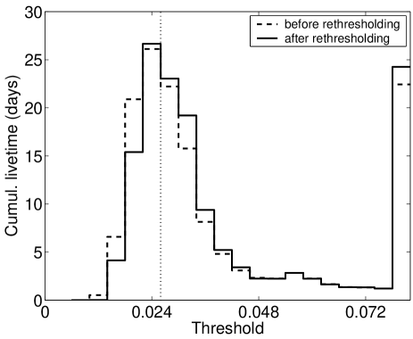
Figure 4: Integrated live time at each discrete threshold. The distribution has a long tail extending beyond the range shown here; this tail has been added to the last bin of the figure. The threshold step size is 0.004. The four values from 0.012 to 0.024 (left of the vertical line) are considered “quiet” and used for the present analysis. Including data taken at larger thresholds would increase the background while negligibly increasing neutrino exposure. The dashed and solid histograms represent the same quantity before and after, respectively, the offline re-thresholding described in the text.

The frequency response of the hydrophone/amplifiers chain is flat to better than 8 dB between 7.5 kHz and 50 kHz. A sharp cutoff of 100 dB/octave below 7.5 kHz is due to an analog high pass filter in the system, while a somewhat slower roll-off, due to the sensor itself, occurs above 50 kHz. The low frequency cutoff, while not ideal for neutrino detection, is not a significant hindrance.

The phase response of the hydrophone/amplifiers chain is difficult to measure and at present is not well known. In order to gain some quantitative understanding of its possible effects on the trigger, the efficiency of the filter was calculated for the pulse shapes in Figure 2 and for their first and second time derivatives, after applying a 9th-order Butterworth bandpass filter to mimic the AUTEC frequency response. For each of these phase responses, efficiency was calculated as a function of energy. The resulting trigger thresholds have a spread of a factor of two for any given energy. Conservatively, the highest of these thresholds is assumed in the present analysis.

In addition to the matched filter described above, an online veto is applied to remove a specific kind of noise that is time-correlated in all channels. This noise consists of simultaneous sinusoids in all 7 channels, occurring in bursts with a 60 Hz repetition rate. While the origin of these signals is unknown, it is clear that they originate from electrical pickup, because the sound velocity does not allow for simultaneous, correlated acoustic events in all phones. The veto removes this noise by rejecting events with large 7-channel pairwise correlation,

$$C=\sum_{i<j}\sum_{t}p_{i}(t)p_{j}(t),$$ (2)

where the time sum is taken over discrete samples and $p_{i}$ is the pressure time series at phone $i$, normalized by mean absolute amplitude: $p_{i}=P_{i}/\langle|P_{i}|\rangle$ where $P_{i}$ is the absolute pressure and $\langle|P_{i}|\rangle$ is its average over the captured waveform. Events with $C>500$ are removed.

Every 10 minutes, time series for all channels are collected for 100 ms in forced mode. These data are used for offline noise analysis and for simulating the noise conditions in our efficiency calculation. Every minute the noise spectrum is calculated from a 100 ms-long time series. A typical noise spectrum is given in Figure 5.

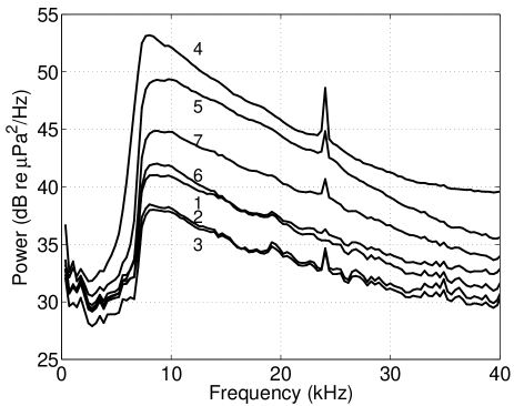
Figure 5: A typical average noise spectrum as measured by SAUND in Run B. The plot shows the spectrum averaged over 10 hours from midnight to 10:00 AM on Dec. 22, 2001. The range of noise levels is mainly due to variations in amplifier gains. Note the 7.5 kHz high-pass filter and the $\sim 24$ kHz peak from a transmitter used by the Navy. The sea state noise dominates these spectra.

SAUND Run B provides the largest data set ever collected for the purpose of studying acoustic techniques in UHE particle detection. During the run it has been our strategy to collect data with consistent and stable conditions for an extended period of time. A number of improvements in trigger efficiency, stability and uniformity have been developed from Run B and will be implemented in future runs.

III Energy and Position Calibration

Small implosions are useful calibration sources for underwater acoustics. Household light bulbs, which implode at a particular failure pressure while sinking, releasing energies of order 100 J  , are a particularly convenient source (Heard et al., 1997). A calibration run of this type was performed on the morning of July 30, 2001 (at the beginning of Run A).

The small boat used for the calibration was positioned over the central hydrophone using a handheld Global Positioning System (GPS) receiver. The boat engine was then turned off and several light bulbs were sunk as the vessel drifted for about thirty minutes. Two more GPS fixes were acquired during the calibration.

The waveforms recorded for one of the implosion events are shown in Figure 6. The first pulse corresponds to the direct acoustic signal arriving at the central hydrophone. The pulse around 0.2 s corresponds to the arrival at the hydrophone of the signal reflected by the surface of the ocean. Direct pulses in all other six hydrophones appear between 0.4 s and 0.5 s, followed, in turn, by the respective surface reflections. In Figure 7 the waveform for the central hydrophone is shown on an expanded time scale, clearly showing the bottom reflection around 6 ms.

Also shown in Figure 7 is the structure of the direct pulse. The signal is expected to be a damped sinusoid, generated by the “breathing” oscillations of the gas bubble produced by the bulb. In our case, the primary resonant frequency of the bubble, at a depth of 100-200 m depth, is predicted to be 700-1300 Hz (Heard et al., 1997). The signal shown in Figure 7 shows a second peak at about 1 ms, confirming this prediction. The measured waveform is consistent with the predicted waveform after a 7.5 kHz high-pass filter.

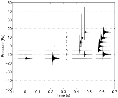
Figure 6: Signals from a light bulb implosion. Time series from all seven hydrophones are shown. A direct signal at the central hydrophone is immediately followed by a bottom reflection and, much later, by the signal from the reflection off the ocean surface. Similar sets of 3 signals appear, at a later time, on the surrounding six hydrophones. The signals in different channels are displaced vertically for clarity. The small signal in phone 1 at $t=$ 0 is electrical cross-talk due to the large signal in phone 7.

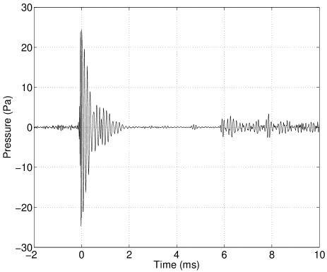
Figure 7: Detail of the light bulb implosion signal at the central hydrophone. Both the direct signal and, after a 6 ms delay, the bottom reflection, are evident. The oscillations in the envelope of the direct signal are due to a combination of the bubble rebound from the implosion (Heard et al., 1997) and the response of the hydrophone, cable and amplifiers.

A time-difference of arrival (TDOA) (Spiesberger, 2001) analysis can be used to reconstruct the 3D location of acoustic events. This method uses only timing information. In a homogeneous medium, the difference in arrival times between each pair of hydrophones constrains the source location to a hyperboloid. Four hydrophones (three independent time differences) are necessary to determine three hyperboloids, the intersection of which can be found analytically and generally results in two points. For our sea-floor, planar array, the two solutions are usually symmetric about the detector plane, and the solution below the sea floor can be discarded.

While an analytical TDOA solution is possible in homogeneous media, the ocean is not homogeneous but is a layered medium. At AUTEC, the sound velocity varies with depth as shown in Figure 8. This results in sound ray refraction as illustrated in the same Figure. Over the fiducial volume of the SAUND detector refraction significantly affects position reconstruction. The effect warps the TDOA hyperboloids, making an analytical solution impossible. A numerical solution is sought by minimizing the metric

$$m(\vec{s})=\frac{1}{N-1}\sum_{i<j}\left[t_{ij}^{meas}-t_{ij}(\vec{s})\right]^{2}$$ (3)

with respect to $\vec{s}$, the test location for the acoustic source. Here $t_{ij}^{meas}$ is the measured TDOA between phones $i$ and $j$ ($t_{ij}^{meas}=t_{i}^{meas}-t_{j}^{meas}$) and $t_{ij}(\vec{s})$ is the theoretical difference in arrival times for a source at $\vec{s}$ ($t_{ij}(\vec{s})=t_{i}(\vec{s})-t_{j}(\vec{s})$). For $N$ phones recording a signal, the sum occurs over the $N-1$ independent pairs of arrival time differences.

The theoretical travel time from the test source location to phone $i$, $t_{i}(\vec{s})$, is calculated using a ray trace algorithm that divides the water into layers in each of which the sound speed is a linear function of depth. The ray follows the arc of a circle within each layer (Boyles, 1984). Practically, the ray trace is too time intensive to be performed for each test source location. For each phone, a table of travel times from points on a grid spanning the detector volume to the phone is built. The minimization begins at the best grid point, and the grid is linearly interpolated to find the off-grid source location. The grid is built once, and the interpolation then occurs for each event reconstruction. While the local sound velocity profile (SVP) is measured almost daily by the Navy and is available to us, it was found that seasonal SVP variations introduce errors smaller than those due to the uncertainty in the hydrophone location. Hence a single table built from an average SVP is used for all reconstructions. The position reconstruction algorithm takes a few seconds to run, for each localization, on a 1.6 GHz Athlon CPU (offline computer).

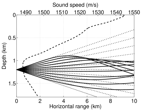
Figure 8: Example of ray trace showing the effects of refraction. 11 rays are emitted from a source at 1200 m depth, from $5^{\circ}$ below to $5^{\circ}$ above the horizontal. Refracted (solid) and unrefracted (dotted) rays are plotted together for comparison. For reference, the sound speed as a function of depth (“sound velocity profile”, SVP), used to calculate the ray trace, is also shown (dashed).

Because the light bulb implosions are far above noise, their TDOA localization is performed using all 7 direct signals (6 independent time differences), rather than 5 as used for events triggered in neutrino mode. The reconstructed depth of bulb failure, $D$, is then used to estimate the energy released in the implosion, $P_{\rm amb}V$. Here $P_{\rm amb}=\rho gD$ is the ambient pressure at the reconstructed implosion depth, $\rho$ is the approximate density of sea water ($\rho=1$ g/cm³), $g$ is the acceleration due to gravity, and $V\sim 150$ cm³ is the volume of the light bulb. From our position reconstruction $P_{\rm amb}$ is found to be of order 1000 kPa, while the internal pressure of the bulbs is believed to be slightly below one atmosphere (70-90 kPa (Heard et al., 1997)). The total acoustic energy detected at phone $i$, $E_{\rm det}(i)$, can be calculated independently assuming spherical emission (Elmore and Heald, 1985):

$$E_{\rm det}(i)=\frac{4\pi r^{2}}{\rho c}\int P^{2}(i,t)dt,$$ (4)

where $P(i,t)$ is the recorded pressure time series at phone $i$, and $r$ is the distance from phone to reconstructed implosion location. Lensing effects due to the changing sound velocity as a function of depth were studied and found to be negligible for these source locations.

The horizontal reconstructed positions of the light bulb implosions are shown in Figure 9, along with the three GPS fixes of the boat from which they were dropped. The implosions are sequentially numbered in the order they occurred. The GPS points, shown with the $\pm 15$ m errors quoted by the specifications of the instrument, are in good agreement with the TDOA reconstruction. The extent of the drift is consistent with a current of about 5 cm/s (0.1 knot).

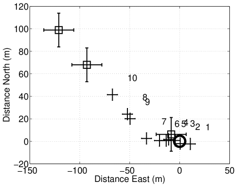
Figure 9: The trail of implosions of bulbs dropped from a drifting boat, as reconstructed from time-differences of arrival. The reconstructed positions are indicated by crosses, with bulb labels offset for clarity. The boat’s motor was cut after starting approximately above the central hydrophone (marked by a circle). The larger crosses represent the boat positions measured at three times with the GPS device. Bulbs are numbered by the order in which they were dropped. The bulb drop spanned one half hour.

The results of depth and energy reconstruction for the implosions are shown in Table 1. The uncertainty of position reconstruction near the surface directly above the center of the array (the optimal location for source localization) is 5 m. The implosion pressures $P_{\rm amb}$ are consistent with the literature (Heard et al., 1997). The efficiency of conversion from $P_{\rm amb}V$ to acoustic energy is expected to be about 4% (Heard et al., 1997). In addition the acoustic frequency spectrum from the implosion is known to be peaked around the air bubble resonant frequency of $\sim 1$ kHz, well below AUTEC’s low frequency cutoff (Gaitan et al, 1992; Keller & Kolodner, 1956; Keller & Miksis, 1980), so that only about one-half of the acoustic energy lies within AUTEC’s bandwidth. The expected energy, taking into account both the 4% yield and the bandwidth mismatch, is shown in column 5 of Table 1. From energy reconstructed using recorded amplitudes (column 6), we find that the yield is in practice somewhat lower and it fluctuates substantially from one event to another. Both these effects are possibly due (Heard et al., 1997) to the fact that the bulbs are allowed to implode at failure pressure rather than being intentionally broken at lower ambient pressure.

Table 1: Parameters of the implosion calibration events. $D$ is the reconstructed implosion depth and $P_{\rm amb}=\rho gD$ is the ambient pressure at $D$. Here $\rho\simeq 1$ g/cm³ is the density of sea water and $P_{\rm amb}V$ is the implosion energy, with $V=~{}150~{}\rm cm^{3}$ the bulb volume. $E_{\rm theor}$ is the theoretical detectable acoustic energy, assuming 4% conversion of the energy $P_{\rm amb}V$, as appropriate for implosions triggered with a hammer device (Heard et al., 1997). $E_{\rm theor}$ includes the effects of absorption and SAUND’s frequency response. The somewhat lower yield observed ($E_{\rm det}$) is consistent with the expectation of lower acoustic coupling for implosions allowed to occur at failure pressure rather than forced at lower pressure with a hammer device (Heard et al., 1997).

Bulb	$D$	$P_{\rm amb}$	$P_{\rm amb}V$	$E_{\rm theor}$	$E_{\rm det}$
	(m)	(kPa )	(J)	(J)	(J)
1	170	1640	250	3.1	1.7
2	110	1120	170	1.9	0.3
3	150	1430	210	2.6	1.5
4	170	1690	250	3.2	2.8
5	130	1300	200	2.3	0.8
6	110	1050	160	1.8	0.4
7	90	900	140	1.5	0.1
8	140	1380	210	2.5	1.9
9	200	1930	290	3.8	1.9
10	300	2930	440	6.7	1.8

IV Data Reduction

The online trigger system is designed to select impulsive bipolar signals while rejecting most of the Gaussian noise. Because of the novelty of the technique, trigger conditions are chosen to be rather loose and substantial background is left to be rejected by off-line analysis. Impulsive backgrounds to UHE showers are expected to arise from a variety of human and non-human sources. In particular a number of animals, from large cetaceans to small crustaceans, are known to produce high-frequency acoustic transient noises. While the Tongue of the Ocean is relatively isolated from the open ocean and hence rather quiet, an important motivation for this first large-volume data-taking campaign is the exploration of such coherent backgrounds.

Offline data reduction is used to select events consistent with neutrino-induced showers while rejecting backgrounds in SAUND Run B. The efficiency of each step of data reduction is estimated using simulated neutrino events to which, as discussed above, bandpass filtering is applied to account for the known frequency response of the array. As is also described above, the unknown phase response of SAUND is addressed by repeating the efficiency analysis with the first and second derivative of the simulated and filtered signal. The worst case (lowest efficiency) is then assumed. The overall efficiency of the data reduction cuts is $>0.87$ and is approximated as 1. The data-reduction power of each analysis cut is shown in Table 2.

The first step in offline data analysis is a set of data quality cuts. These are particularly important because of the volatility of the background noise. The adaptive thresholding algorithm used online was in some cases found to be too slow in reacting to the changing conditions. Hence, offline re-thresholding is applied by raising the threshold whenever the rate exceeds 60 events/min (see Figure 4). The cut selecting “quiet” events is applied using the threshold values after re-thresholding. Finally, events with $\Delta t_{0}<$ 1 ms are removed, where $\Delta t_{0}$ is the difference in time stamps between the current event and the previous one. This last cut rejects bursts of events that occasionally occur when the threshold has not adapted sufficiently and is too low. The combination of all event quality cuts reduced the Run B data set from 20.2 million to 2.56 million events, with an estimated neutrino efficiency of $>99\%$ (counting the “quiet” cut as a livetime reduction, not an efficiency reduction).

Table 2: Event rates at different stages of online (1) and offline (2-5) data reduction. Note that the cuts in 1-3 are applied to single-phone events, while the cuts in 4 are applied to coincidences between 5 phones. The “Events” column gives the number of events surviving a particular cut and all the preceding ones. Cut 4a includes both coincidence windowing and hit-phone geometry (requiring the set of 5 hit phones to be one of the 6 trapezoidal configurations). Finally Cut 5 requires the sources to be in the geometrical region consistent with neutrino showers and it eliminates all remaining events.

Cut	Description	Events
1)	Online Triggers
	a) digital filter	64.6 M
	b) correlated noise	20.2 M
2)	Quality Cuts
	a) offline re-thresholding	7.23 M
	b) offline quiet conditions	2.60 M
	c) $\Delta t_{0}>$ 1 ms	2.56 M
3)	Waveform Analysis
	a) remove spikes	2.03 M
	b) remove diamonds	1.96 M
	c) $f_{e}>$ 25 kHz	1.92 M
4)	Coincidence Building
	a) coincidence	948
	b) localization convergence	79
5)	Geometrical fiducial region	0

Waveform analysis is then used to further reduce the background. A powerful method of event classification is provided by the scatter plot between effective frequency $f_{e}$ and duration, measured in effective number of cycles $n_{e}$. We define the effective frequency as

$$f_{e}={\frac{1}{2\pi\Delta t}}\cos^{-1}\left[{\frac{\langle P(t)P(t+\Delta t)\rangle}{\langle P^{2}(t)\rangle}}\right],$$ (5)

where $P(t)$ is the recorded pressure time series and $\Delta t$ is the sampling time (5.6 $\mu$s), small compared to the signal oscillation period. The effective duration in number of cycles is given by $n_{e}=D_{e}f_{e}$, where

$$D_{e}=\frac{E_{S}}{\frac{1}{2}P_{\rm peak}^{2}}$$ (6)

is the duration of the signal in units of time. Here $P_{\rm peak}$ is the maximum absolute amplitude of the recorded time series and

$$E_{S}=E_{S+N}-E_{N}=\int P^{2}(t)dt-\int P_{\rm rms}^{2}dt,$$ (7)

where $P_{\rm rms}$ is determined from the noise spectrum calculated once per minute. The normalization is such that a sinusoid, in the limit of many periods in the capture window, will give $n_{e}$ equal to the number of cycles of the sinusoid. The contour plot between these two parameters is shown in Figure 10 for the 2.56 million events left in the data set. Also shown in Figure 10 is the envelope of the regions containing $\sim 95$ % of the neutrinos simulated, filtered and differentiated as described above.

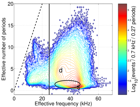
Figure 10: Contour plot between effective frequency and effective number of periods, as defined in the text. The dashed line represents an upper bound due to the finite length of the capture window (1 ms). The events clustered near this line are due to Navy pingers at specific frequencies. The solid vertical line indicates a cut discussed in the text. The ellipse indicates the envelope of approximate locations of the simulated neutrino events with different combinations of filtering and differentiation as discussed in the text. The letters “s” and “d” identify regions where “spike” and “diamond” -type events cluster.

The general region marked “s” in the contour plot includes events, here called “spikes,” in which a single digital sample is displaced from the rest of the waveform. Spike events occurred in bursts with a 50 Hz rate and ceased when a large radar system near our DAQ system was disabled. We reject spike events with the metric

$$m_{\rm spike}=\frac{M_{1}(|P|)-M_{2}(|P|)}{M_{1}(|P|)}$$ (8)

where $P$ is the pressure time series and $M_{1}$ and $M_{2}$ give the largest and second-largest amplitude samples, respectively. Events with $m_{\rm spike}<0.7$ are retained.

The region of Figure 10 marked “d” includes events, here called “diamonds,” consisting of a diamond-shaped envelope containing many cycles. These events, an example of which is shown in the top panel of Figure 11, are believed to be genuine acoustic signals produced by marine mammals swimming in the area. They can be rejected with a digital matched filter whose response function was constructed by averaging 10 hand-picked examples of good diamond events. The diamond rejection metric, $m_{\rm diamond}$, is defined for a given waveform to be the maximum output of this digital filter acting on the waveform. Events with $m_{\rm diamond}<0.7$ are retained.

Finally, neutrino candidates are required to have $f_{e}>25$ kHz. This cut eliminates low-frequency noise originating from sources including marine mammals, boats, and AUTEC pingers.

Waveform analysis reduces the data set from 2.56M to 1.92M events, retaining $\sim 93\%$ of the simulated neutrino events.

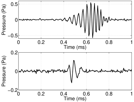
Figure 11: Waveforms of two important classes of background. Upper panel: “diamond” events. They are easily rejected with a digital matched filter. Lower panel: “multipolars.” Depending on the phase response of the SAUND detector, multipolar events could be indistinguishable from neutrino signals.

Coincidences between different hydrophones are reconstructed from the reduced data set. The reconstruction program first finds cases in which 5 different phones trigger within a 2.27 s coincidence window. This window is the maximum possible time delay between phones plus a 10% buffer to account for measurement errors and refraction. We then require that the 5 events satisfy causality pairwise, a more stringent requirement than the initial windowing, again with a 10% buffer. Finally we apply a phone geometry cut: There are 21 ways to choose 5 of the 7 phones. 6 of these combinations, those forming a trapezoid, are consistent with a pancake radiation pattern triggering all phones enclosed by the pattern. Only coincidences triggering one of these 6 5-phone combinations are retained.

These timing and geometrical cuts greatly reduce the data set, from 1.92 million to 948 events, retaining an efficiency of $95\%$ for neutrino events. Such a substantial data reduction is essential in order to perform the computationally intensive origin localization with TDOA in a layered medium. A given single-phone trigger may be included in several (even many) 5-trigger coincidences. This is because coincidence is a much less powerful requirement for acoustic signals than for electromagnetic signals, because the propagation speed is $2\times 10^{5}$ times lower. While only four phones are required for TDOA localization, 5-phone coincidence is demanded, both to over-constrain the reconstruction and to reduce the background, without significantly decreasing the neutrino efficiency.

For most coincidences, TDOA does not converge on a consistent solution to the causality equations (solved numerically, accounting for refraction with ray-trace tables). These coincidences are presumably accidental and are therefore discarded. Most of the 79 events remaining in our data set have “multipolar” waveforms at more than one of the 5 phones triggered. It is apparent that this class of events may be difficult to separate from genuine neutrino signals on the sole basis of pulse-shape properties. To explore the properties of multipolar events we have built a digital matched filter using the average of 11 waveforms from events manually chosen as good examples of this event type. By applying the matched filter to earlier stages of the event selection it was found that multipolar events tend to accumulate in periods of large adaptive threshold, and many such events in the original data set are rejected by the “quiet conditions” (2b) cut. Clearly a full pulse-shape calibration, including phase, of the acoustic sensors and their readout chain will be essential for future detector arrays. For the present data set we conservatively do not use the multipolar event digital filter. As will be shown in the next section, geometrical considerations make all of these events inconsistent with a neutrino origin.

V Acceptance Estimate

The Monte Carlo (MC) simulation used to estimate the detector efficiency is run for a set of discrete primary neutrino energies. For each energy, detection contours, examples of which are given in Figure 12, are calculated by determining the pressure pulse at each point in space (accounting for attenuation) and then applying the digital filter. For each energy $N_{\rm MC}=10^{5}$ simulated neutrino events are produced with random orientations and positions in a water cylinder of radius 5 km, centered around the central phone. The detection contour is then “bent” to account for refraction and its intersection with the different phones in the array is tested as shown, for a particular configuration, in Figure 13. For an energy $E$ the acceptance is then given by $A_{i}(E)=A_{0}N_{i}/N_{\rm MC}$, where $N_{i}$ is the number of Monte Carlo events producing five or more hits at the threshold value identified by $i$. $A_{0}=\Omega_{0}V_{0}$ is the acceptance that would result if all $N_{\rm MC}$ events were detected, where $\Omega_{0}$ is the total solid angle, and $V_{0}$ the total volume within which events are chosen.

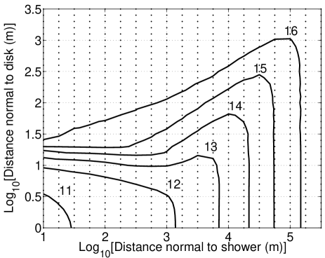
Figure 12: Neutrino detection contours for SAUND, for a trigger threshold of 0.02. In the plot the neutrino producing the shower propagates along the vertical axis. The shower maximum is at the origin of the coordinate system. Curves are labeled by $\log_{10}[E({\rm GeV})]$. Only one quadrant is represented.

Although the outer hydrophones are only 1.5 km from the central one, it was found that events with the appropriate orientation can safely be detected and localized up to a radial distance of 5 km. Outside of this region, however, the rays reach vertical turning points and precise source localization becomes difficult. For this reason, we conservatively limit the fiducial volume to 5 km radius. The requirement that the radiation pancake intercepts several hydrophones almost coplanar with the sea floor forces the direction of the accepted neutrinos to be close to the vertical.

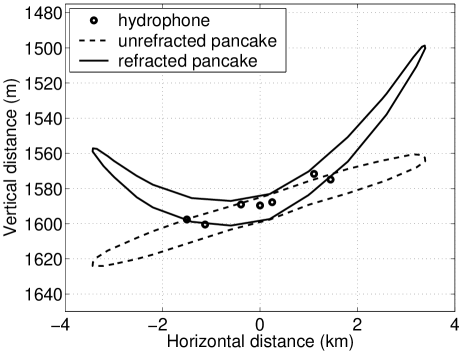
Figure 13: The effect of refraction on the acoustic radiation envelope (pancake). A cross section of the acoustic radiation pattern from a $3\times 10^{21}$ eV neutrino at $0.5^{\circ}$ zenith is shown with and without refraction. Projections of the seven hydrophone locations onto the cross sections are shown for reference. Note that the detector is inclined to $\sim 0.5^{\circ}$ zenith, $7^{\circ}$ east of north, due to the slightly sloping sea floor.

The uncertainty in source position reconstruction, estimated from Monte Carlo data, worsens steadily with distance outside the array, but it does not exceed 500 m (vertical) and 200 m (horizontal) for radial distances smaller than 5 km. The positions of detectable neutrino Monte Carlo events with energies of $10^{14}$ GeV, $10^{15}$ GeV, and $10^{16}$ GeV are shown in a side (top) view in Figure 14 (Figure 15). The concentration of events slightly above the plane defined by the phones is consistent with the geometrical considerations above. The positions of the 79 acoustic events passing all analysis cuts (except for fiducial volume) in Run B are also shown as small squares. There is a clear separation between these events, mainly concentrated in the water column above the hydrophones, and the region where the neutrino events are expected to be. Hence, we conclude that the spatial distribution of the observed events is incompatible with the one expected from neutrino interactions. The expected pancake shape of the acoustic emission profile from neutrinos is an essential assumption of this assertion.

Focusing effects can potentially alter the detected energy and hence the threshold value. As shown in Figure 16, such focusing effects are small for sources in the neutrino fiducial volume and are neglected.

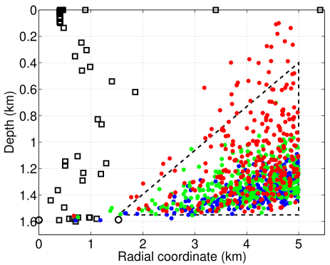
Figure 14: Side view of reconstructed positions (squares) for the 79 coincidences surviving all cuts except for fiducial volume. The event with greatest radial coordinate is that at 5.4 km (no events occur beyond the plot boundary). The fiducial volume is bounded by the dashed triangle. Circles represent hydrophone positions. 300 neutrino Monte Carlo events are also plotted, as colored dots, for each of three different energies, $10^{14}$ GeV (blue), $10^{15}$ GeV (green), and $10^{16}$ GeV (red).

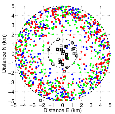
Figure 15: Top view of the reconstructed positions (squares) for the 79 acoustic neutrino candidates surviving the selection cuts. The fiducial volume is bound by the two dashed circles. The small circles represent the positions of the hydrophones. Neutrino Monte Carlo events for three different energies are also shown with the same convention as in Figure 14.

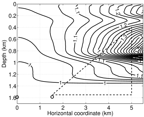
Figure 16: Degree of acoustic flux focusing at the central hydrophone, for sources at various points as calculated from ray tracing (Boyles, 1984). Contours of equal focusing are given. The dashed curve encloses the fiducial volume used for the neutrino analysis. Central and peripheral hydrophone locations are indicated by circles. Factors greater than one indicate focusing.

In order to express this result as an upper limit to the ultra high energy neutrino flux, we define a fiducial volume given by the revolution of the dashed triangle around the vertical axis. The fiducial region is chosen to be slightly above the ocean floor in order not to be affected by floor roughness. Ideally, the fiducial volume choice would have been based entirely on the signal Monte Carlo events. However, given the novelty of the technique and the present emphasis on studying backgrounds, such a “blind” approach is impractical here. The separation between expected neutrino region and observed coincidences is nevertheless striking enough that the definition of the fiducial volume is unambiguous. In fact, the main source of uncertainty in our analysis lies in the assumptions made about the phase response of the array. No 5-phone coincidences are present in SAUND Run B within the fiducial volume.

From the geometrical acceptance $A_{i}(E)$ defined above, a “neutrino exposure” $X_{i}(E)=A_{i}(E)N_{A}\sigma(E)T_{i}$ is computed. Here $N_{A}$ is the Avogadro number, $\sigma(E)$ is the neutrino cross section and $T_{i}$ is the live time for a particular value of the adaptive threshold, labeled by $i$. $\sigma$ is estimated by extrapolating the power-law fit given for energies between 10¹⁶ eV and 10²¹ eV in (Gandhi et al, 1996). Fits for neutrinos are used, the anti-neutrino fits being very similar. Exposures collected at different thresholds are then added together. A 90% CL flux limit is then calculated following the method of Ref. (Lehtinen et al., 2004) using Poisson’s statistics and the fact that no events are observed. The resulting limit (multiplied by $E^{2}$, as customary) is shown in Figure 17 along with the limits already available from FORTE (Lehtinen et al., 2004), RICE (Kravchenko et al., 2003) and GLUE (Gorham et al., 2003), and with fluxes predicted by various theories (Weiler, 2001; Gelmini & Kusenko, 2000; Fodor et al., 2002; Waxman & Bahcall, 1997; Hill & Schramm, 1985; Sigl et al., 1999).

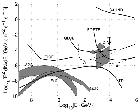
Figure 17: Diffuse neutrino flux limit from SAUND and other experiments and theoretical models of neutrino fluxes. The SAUND limit is the solid curve on the top-right. The hypothetical sensitivities of two different optimized acoustic arrays (A and B), described in the text, are shown as dashed curves. Other experimental limits (FORTE, GLUE, and RICE) are shown in solid black. The remaining curves and regions indicate various theoretical models: “Z” for Z-bursts (one large trapezoid, three small quadrilaterals, and arrow), “TD” for topological defects, “AGN” for active galactic nuclei, “GZK” for GZK neutrinos, and “WB” for the Waxmann-Bahcall limit.

VI Discussion

While the main motivation of this work has been to gain operational experience and investigate acoustic backgrounds for UHE neutrino detection, a flux measurement was obtained from the data. Although the limit, shown in Figure 17, is not competitive with the best limits (obtained with radio techniques) it represents the first UHE neutrino measurement performed with acoustic techniques. A wealth of information on noise conditions and the possible methods available to separate such noise from the neutrino signals has been obtained. Here we briefly discuss the characteristics of the SAUND array that turned out to be sub-optimal for UHE neutrino detection, and we describe some of the properties that an optimized acoustic neutrino array should have.

The importance of calibrating the phase response of the acoustic array cannot be overstated. Without such a calibration, it is expected that the unknown phase properties of the readout will dominate the systematics of the measurement. An artificial source capable of providing acoustic signals similar to those from neutrinos with energies in the range considered here can be realized by discharging a capacitor in a column of sea water of length similar to that of a UHE shower. The instantaneous heating of the water should closely simulate the heating produced by showers, releasing an acoustic wave with the correct pancake geometry and phase/frequency structure.

The flatness of the acoustic radiation lobes from UHE showers is a crucial feature that allows noise rejection but also drastically limits the acceptance of SAUND. Refraction exacerbates the problem, by making regions of sea invisible to the array and by curving the emission pancake into a shape that often has little overlap with a planar hydrophone array. The planar geometry of the SAUND array is also poorly optimized to provide good position resolution in the direction orthogonal to the plane. The vertical resolution is estimated to be as poor as 400 m for sources deeper than 1400 m, while it is 10 m for sources close to the surface. The resolution in the horizontal plane, however, is better than 10 m in most of the volume. A hydrophone array on a 3D lattice would provide substantially larger acceptance and superior pancake-shape identification.

Although the long attenuation length of sound in water allows for large (several hundred meters to several kilometers) horizontal spacing for an optimized neutrino detector, to overcome the flatness of the acoustic radiation an array with dense ($\sim 10$ m) vertical spacing is necessary. Even better, the ideal array would consist not of strings of discrete modules, but of strings sensitive to acoustic signals uniformly along their entire length. Such a detector element is not inconceivable and could perhaps be realized with a tube of fluid of sound speed different from the surrounding water, attached to hydrophones on each end. When an acoustic signal intercepts the tube, the difference in sound speeds leads to a signal propagating in both directions along the tube. The difference in arrival times at the two hydrophones could be used to localize the intersection point. Other possibilities may include interferometers built with an optical fiber running along the length of the string (although is it not clear how this could vertically localize signals).

To explore the possible sensitivity of an array of such strings with dense vertical spacing, two hypothetical arrays were tested with Monte Carlo neutrinos. Both are hexagonal lattices of 367 1.5 km-long strings. The first (“A”) has 500 m nearest-neighbor spacing and is bounded by a circle of radius $R=5$ km drawn about the central string. The second (“B”) has 5 km spacing and is bounded by an $R=50$ km circle. Both are taken to have a fiducial volume given by a cylinder of height 1.5 km and radius $R+5$ km. Circles of various radii representing acoustic radiation from neutrinos of various energies were generated throughout this fiducial volume, with zenith from 0 to $\pi$/2. The calculated sensitivity of these arrays, requiring 5 strings hit, is given in Figure 17.

While water is the first medium to be tested for acoustic neutrino detection, salt (available in naturally-occurring multi-km³ underground domes) and ice (available near the poles in multi-km deep sheets) may be more favorable. In polar ice as compared with ocean water, noise is expected to be significantly lower, and signals are predicted to be greater by an order of magnitude (Price, 1996). It is possible that the hypothetical configurations “A” and “B” above, implemented in ice, possibly with more advanced triggering schemes in which thresholds are lowered for a time window after the first sensor is hit, may allow for better sensitivity at lower energy. Tests are necessary in these media to determine their merit. In any case acoustic detection could be employed in combination with radio and optical Cherenkov techniques to provide more complete information about the very rare events occurring at the highest energies.

VII Acknowledgments

We would like to thank the U.S. Navy and, in particular, D. Belasco, J. Cecil, D. Deveau, and T. Kelly-Bissonnette, for hospitality and help at the AUTEC site. Many illuminating discussions with M. Buckingham and T. Berger (Scripps Institution of Oceanography) are gratefully acknowledged. We thank Y. Zhao (Stanford) for help with the data analysis and N. Kurahashi for a careful reading of the manuscript. One of us (JV) would like to thank M. Oreglia at the University of Chicago for hospitality during part of this work. This work was supported, in part, by NSF Grant PHY0354497 and by a Stanford University Terman fellowship.

References

- Greisen (1966) K. Greisen, Phys. Rev. Lett. 16 (1966) 748;
- Zatsepin & Kuzmin (1966) G.T. Zatsepin and V.A. Kuzmin, JETP Lett. 4 (1966) 78.
- Takeda et al. (1999) H. Takeda et al., Astrophys. J. 522 (1999) 225.
- Abbasi et al. (2002) R.U. Abbasi et al., astro-ph/0208243.
- Bahcall & Waxman (2003) J.N. Bahcall and E. Waxman, Phys. Lett. B556 (2003) 1.
- Gorham et al. (2003) P. Gorham et al., astro-ph/0310232, to appear in Phys. Rev. Lett.
- Kravchenko et al. (2003) I. Kravchenko et al. Astropart. Phys. 20 (2003) 195.
- Lehtinen et al. (2004) N.G. Lehtinen et al. Phys. Rev. D 69 (2004) 013008.
- Askaryan (1957) G.A. Askaryan, Sov. J. Atom. Energy 3 (1957) 921;
- Askaryan & Dolgoshein (1977) G.A. Askaryan and B.A. Dolgoshein JETP Lett. 25 (1977) 213.
- Learned (1979) J.G. Learned, Phys. Rev. D 19 (1979) 3293.
- Sulak et al. (1979) L. Sulak et al., Nucl. Inst. Meth. 161 (1979) 203.
- Lehtinen et al. (2002) N.G. Lehtinen et al., Astropart. Phys. 17 (2002) 279.
- Kwi et al (1999) J. Kwiecinski et al., Phys. Rev. D 59 (1999) 093002.
- Gandhi et al (1996) R. Gandhi et al., Astropart. Phys. 5 (1996) 81.
- Landau & Pomeranchuk (1935) L.D. Landau and I. Pomeranchuk, Dokl. Akad. Nauk USSR 92 (1953) 535; L.D. Landau and I. Pomeranchuk, Dokl. Akad. Nauk USSR 92 (1953) 735;
- Migdal (1956) A.B. Migdal, Phys. Rev. 103 (1956) 1811;
- Migdal (1957) A.B. Migdal, Sov. Phys. JETP 5 (1957) 527.
- Alvarez & Zas (1998) J. Alvarez-Muniz and E. Zas, Phys. Lett. B 434 (1998) 396.
- Hogg & Craig (1995) R.V. Hogg and A.T. Craig, “Introduction to Mathematical Statistics,” ed., Macmillan College Pub. Co., New York, 1995.
- Knudsen et al. (1948) V.O. Knudsen, R.S. Alford and J.W. Emling, J. Marine Res. 7 (1948) 410.
- Heard et al. (1997) G.J. Heard et al. in OCEANS ’97, IEEE Conference Proceedings 2 (1997) 755.
- Elmore and Heald (1985) W.C. Elmore and M.A. Heald, “Physics of waves”, Dover Publications Inc., New York 1985, p.154.
- Spiesberger (2001) See e.g. J.L. Spiesberger, J. Acoust. Soc. Am. 109 (2001) 3076 and references therein.
- Boyles (1984) C.A. Boyles, “Acoustic waveguides : applications to oceanic science,” Wiley, New York, 1984.
- Gaitan et al (1992) D.F. Gaitan et al., J. Acoust. Soc. Am. 91 (1992) 3166;
- Keller & Kolodner (1956) J.B. Keller and I.I. Kolodner, J. Appl. Phys. 27 (1956) 1152;
- Keller & Miksis (1980) J.B. Keller and M. Miksis, J. Acoust. Soc. Am. 68 (1980) 628.
- Weiler (2001) T.J. Weiler, AIP Conf. Proc. 579 (2001) 58, hep-ph/0103023;
- Gelmini & Kusenko (2000) G. Gelmini and A. Kusenko, Phys. Rev. Lett. 84 (2000) 1378;
- Fodor et al. (2002) Z. Fodor, S.D. Katz and A. Ringwald, JHEP 0206 (2002) 046;
- Waxman & Bahcall (1997) E. Waxman and J.N. Bahcall, Phys. Rev. Lett. 78 (1997) 2292;
- Hill & Schramm (1985) C.T. Hill and D.N. Schramm, Phys. Rev. D 31 (1985) 564;
- Sigl et al. (1999) G. Sigl et al., Phys. Rev. D 59 (1999) 043504.
- Price (1996) P.B. Price, Astropart. Phys. 5 (1996) 43.