Long-Lived Triaxiality in the Dynamically Old Elliptical Galaxy NGC 4365: A Limit on Chaos and Black Hole Mass

Abstract

Supermassive black holes in the centres of giant elliptical galaxies are thought to be capable of inducing chaos and eliminating or preventing triaxiality in their hosts if they are sufficiently massive. We address whether this process operates in real systems, by modeling the stellar kinematics of the old elliptical NGC 4365. This galaxy has a mean stellar population age $>12\mbox{$\rm\,Gyr$}$ and is known for its kinematically decoupled core and skew rotation at larger radii. We fit the two-dimensional mean velocity field obtained by the SAURON integral-field spectrograph, and the isophotal ellipticity and position-angle profiles, using the velocity field (VF) fitting approach. The models constrain the system’s intrinsic shape between $0.03$ and $0.5$ effective radii, as well as its orientation in space. We find NGC 4365 to be strongly triaxial ($\langle T\rangle\approx 0.45$) and somewhat flatter than it appears ($\langle c/a\rangle\approx 0.6$). Axisymmetry or near axisymmetry ($T<0.1$) is ruled out at $>95\%$ confidence for $1\aas@@fstack{\prime\prime}6<R<3\aas@@fstack{\prime\prime}2$ ($0.03<R/r_{e}<0.06$), and at $>99\%$ confidence at larger radii. There is an indication of an outward triaxiality gradient. The line of sight is constrained to two narrow bands on the viewing hemisphere. In the most probable orientation the long axis points roughly toward the observer, extending to the southwest in projection. The stellar population age implies that strong triaxiality has persisted for hundreds of dynamical times. This rules out black holes $>3\times 10^{9}\mbox{$\,M_{\odot}$}$, which numerical simulations indicate would either have globally axisymmetrized the galaxy or made the inner several arcseconds spherical. The $M_{\rm BH}$-$\sigma$ relation predicts $M_{\rm BH}\approx 4\times 10^{8}\mbox{$\,M_{\odot}$}$, which would probably not preclude long-lived triaxiality and is consistent with the observations. There must also be an unequal population of direct and retrograde long-axis tube orbits outside the kinematically decoupled core. This, combined with the small isophotal twist, limits the rate of figure rotation (tumbling) about the short axis, and places corotation at $>8$ effective radii. NGC 4365 lends support to a picture in which supermassive black holes, though omnipresent in luminous giant elliptical galaxies, are not massive enough to alter their global structure through chaos.

1 Introduction

There is growing recognition that the dynamical structure of hot stellar systems—elliptical galaxies and the bulges of spirals—is intimately connected with the supermassive black holes that reside at their centres. The most compelling evidence for this connection is the tight correlation between black hole masses and the velocity dispersions of their host galaxies measured far from the black hole. The $M_{\rm BH}$-$\sigma$ relation (Ferrarese & Merritt, 2000; Gebhardt et al., 2000) indicates that central black holes somehow “know” about the properties of their hosts, and has provoked speculation that host dynamics control the growth of the central object (El Zant et al., 2003; Adams et al., 2003). But the exact mechanisms by which this control might be exerted are still obscure.

By contrast, a mechanism by which a central black hole may, in a turnabout move, affect the structure of its host is understood, or at least identified. Important families of regular orbits that pass close to the centre of the system can be rendered chaotic by scattering off the central mass (Lake & Norman, 1983; Gerhard & Binney, 1985; Gerhard, 1986). It has thus been suggested that growth of a black hole can lead to the destruction of bars in spirals (Hasan & Norman, 1990; Norman et al., 1996) or to the elimination of triaxiality in ellipticals (Valluri & Merritt, 1998; Merritt & Quinlan, 1998). In this case, however, what is lacking is direct evidence that this mechanism has played a role in real systems.

When central point masses or density cusps are added to triaxial potentials, box orbits are transformed to stochastic orbits or resonant “boxlets” (Schwarzschild, 1993). Despite some speculation that the loss of boxes would preclude nearly all triaxial equilibria (Merritt, 1996), it is now understood that stochastic orbits can contribute constructively to maintaining the triaxial figure (Schwarzschild, 1993; Merritt & Fridman, 1996). The important questions now focus on the chaotic mixing time scale (Siopis & Kandrup, 2000), and whether, for practical purposes, one can consider there to be many distinct, slowly diffusing, stochastic orbits at each energy, rather than only one such orbit occupying the entire Arnol’d web (Merritt & Fridman, 1996). Studies of individual orbits (Valluri & Merritt, 1998; Poon & Merritt, 2001) as well as evolutionary $N$-body simulations (Merritt & Quinlan, 1998; Sellwood, 2002) agree that the box-orbit region of phase space becomes fully chaotic when the central point mass reaches $\sim 1\%$ of the total system mass. This transition happens somewhat earlier for more elongated figures or steeper cusps. At lower masses, a fully chaotic zone appears over a limited range of energies, affecting a region whose enclosed stellar mass is of order 10 times that of the central object (Poon & Merritt, 2002; Holley-Bockelmann et al., 2002).

The current $M_{\rm BH}$-$\sigma$ relation (Tremaine et al., 2002), coupled with the Fundamental Plane (Djorgovski & Davis, 1987; Dressler et al., 1987), implies that black holes will typically fall about a factor of 10 short of the 1% mass needed to induce global chaos and a major restructuring of the host galaxy. If this is universally the case, triaxiality should persist over long times, and we should expect to find many old, triaxial ellipticals. However, Valluri & Merritt (1998) argue that the threshold for chaos should be proportionally lower in lower luminosity galaxies, which have steeper cusps and shorter dynamical times, and suggest that galaxies fainter than around $M_{B}\approx-20$ should have been axisymmetrized by chaos. Consequently, determining the actual abundance of triaxial systems as a function of luminosity will be an important check on our understanding of the masses of black holes and their influence on their hosts.

Determining the true shapes of elliptical galaxies cannot be done by photometry alone. Kinematic data are essential (Binney, 1985; Franx et al., 1991), and the “traditional” major and minor axis kinematic profiles are not enough. Statler (1994a) advocated a minimum of 4 long-slit position angles for a credible constraint on triaxiality, a requirement that is prohibitively costly in telescope time. Happily, this has become a moot point with the advent of integral-field spectrographs. The SAURON instrument (Bacon et al., 2001) was developed specifically to map the kinematic and spectral properties of galaxies, with full two-dimensional coverage on the sky. SAURON has been used to observe a sample of 72 E, S0, and Sa galaxies (de Zeeuw et al., 2002), producing an extensive catalog of kinematic and line-index measurements. In this paper we fit triaxial models to the SAURON kinematic dataset for the old elliptical NGC 4365, in order to estimate its intrinsic shape and constrain its orientation relative to the line of sight.

The properties of NGC 4365 have recently been summarized by Davies et al. (2001). It is a luminous giant elliptical ($M_{B}=-21.05$ for a distance modulus of $31.55$) with a very shallow central cusp. The negative logarithmic slope of the inner surface brightness profile is $\gamma\approx 0.13$ (Rest et al., 2001). Photometrically, the galaxy has near-constant ellipticity $\epsilon\approx 0.26$, and a modest isophotal twist of about $10\mbox{${}^{\circ}$}$ from $0.02$ to 2 effective radii ($r_{e}=57\arcsec$). The isophotes are discy in the inner $4\arcsec$ and boxy farther out. NGC 4365 is probably best known for its kinematics, having both a kinematically decoupled core and skew rotation at larger radii. The apparent rotation is about the photometric minor axis in the core, and $\sim 40\mbox{${}^{\circ}$}$ from the major axis at $20\arcsec$ from the centre. These kinematic signatures were recognized by Surma & Bender (1995) as hallmarks of triaxiality. From the SAURON line index maps, Davies et al. (2001) determine that the stellar population in NGC 4365 has a mean age of $14\mbox{$\rm\,Gyr$}$, both in and outside the kinematically distinct core, with at most a few percent admixture of an intermediate-age population in the innermost $1\aas@@fstack{\prime\prime}6$. They find that putting 6% of the mass in a 5-Gyr-old population with the same metallicity as the rest of the galaxy can account for the slightly elevated central H$\beta$ line-strength. Davies et al. (2001) conclude that the galaxy has been largely unchanged in the last $12\mbox{$\rm\,Gyr$}$. However, there is also evidence of a population of intermediate-age (2–8 Gyr old) globular clusters (Puzia et al., 2002; Larsen et al., 2003), suggesting that a minor merger event a few billion years in the past may have modified the structure of the galaxy and possibly contributed to the kinematically decoupled core.

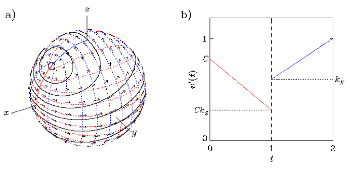
Figure 1: Construction of a velocity field on one fiducial shell. ($a$) A confocal coordinate system linked to the model triaxiality (in this example $T=0.5$) represents the streamlines of short-axis tubes (red dotted lines) and long-axis tubes (blue dotted lines). Given a density distribution, specifying the velocity crossing an arc in the $(x,z)$ plane (heavy colored line) then determines the mean flow field everywhere (black vectors and streamlines). The boundary arc is divided into two segments (red, blue) describing the contribution of short-axis and long-axis tubes, respectively. ($b$) The function $v^{\ast}(t)$, which determines the velocity along the boundary arc, showing the definition of the constants $C$, $k_{X}$, and $k_{Z}$. The example in ($a$) has $C=1$, $k_{X}=k_{Z}=0$.

In § 2 below we describe the methods we use to constrain the shape and orientation of the galaxy, including the nature of the models, the handling of the observational data, and the statistical formalism. § 3 presents the basic results. We find that NGC 4365 is highly triaxial, with axisymmetry ruled out at better than 99% confidence between approximately $2\arcsec$ and $30\arcsec$. We find the line of sight to be constrained to two fairly narrow strips on the hemisphere of viewing angles. We are also able to constrain, to a limited degree, the contributions of the main tube orbit families to the mean velocity field. In § 4 we show that the persistent triaxiality of this old system rules out black holes larger than a few $10^{9}\mbox{$\,M_{\odot}$}$, but is probably consistent with predictions of the $M_{\rm BH}$-$\sigma$ relation. We also use the predominance of long-axis tubes in the outer part of the system and the lack of a strong photometric twist to limit the rate of figure rotation. We briefly discuss the implications for orbit-based (Schwarzschild) and moment-based (Jeans) models, before summarizing the principal results in § 5.

2 Method

We determine the intrinsic shape of the galaxy by fitting models to the mean line-of-sight velocities and the radial profiles of isophotal ellipticity and major-axis position angle. We do not make use of the dispersion or the higher moments (except for a $v/\sigma$ constraint described below), because our goal is not to determine the full three-dimensional mass profile. That is a job better left to the more sophisticated—but far slower—Schwarzschild method. Our goal is only to constrain the shapes of the isodensity surfaces and the orientation of the galaxy relative to the line of sight. We can extract this information from the mean rotation and photometry because the mean velocities in a non-tumbling triaxial galaxy arise from the populations of stars on short-axis (Z) and long-axis (X) tube orbits, and the geometry of these orbits is determined almost entirely by the triaxiality of the potential.

2.1 Models

The velocity field (VF) fitting approach has been described in previous papers (Statler, 2001; Statler et al., 1999, and references therein). The models are based on analytic solutions to the equation of continuity. Though the models are approximate, their calculation is extremely fast, making it possible to explore a far larger parameter space than can be covered by more computationally intensive orbit-based methods. We sketch the essentials here, and explain certain details in the Appendix.

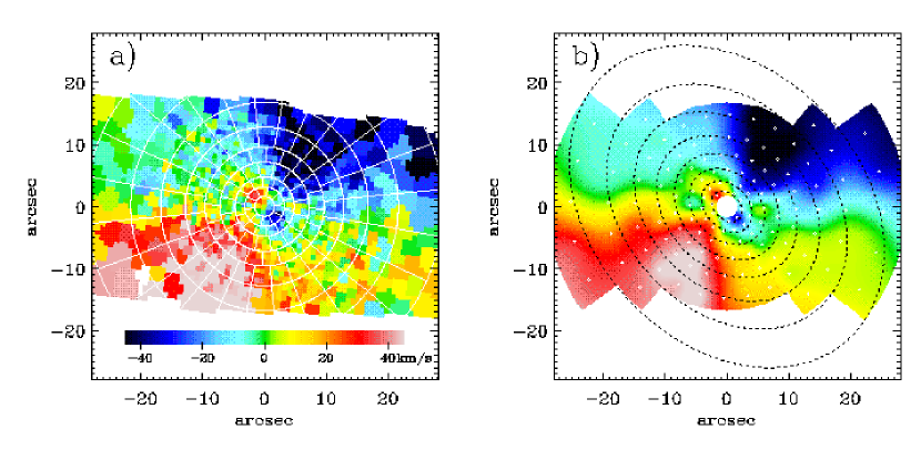
Figure 2: ($a$) SAURON mean velocity field for NGC 4365. Velocities are computed from spectra averaged over Voronoi cells, and are corrected for the $h_{3}$ Gauss-Hermite term inside $R=7\aas@@fstack{\prime\prime}2$. The color bar indicates the velocity scale relative to systemic. Overplotted “spider web” shows the polar grid on to which the data are rebinned for model fitting. ($b$) Rebinned velocity field, antisymmetrized by folding and averaging points on opposite sides of the centre. White points mark the bin centres. Colors show a continuous velocity field interpolated from the rebinned data. The whited-out central region is excluded from the fit. Dotted lines show $V$-band isophotes. This and all similar figures have North up and East to the left.

The figure of the galaxy is assumed to be stationary, and the principal axes of the isodensity surfaces are assumed to be aligned throughout. For each projected radius at which there are data to be fitted, we calculate an internal (3-dimensional) mean VF by solving the equation of continuity on a deprojected shell. This solution involves the assumed density figure of the model as well as the geometry of the streamlines of the mean flow. To approximate the latter, we assume that the mean motions (not the single-particle orbital velocities) of X and Z tubes follow coordinate lines in a confocal coordinate system that is keyed to the triaxiality $T$ of the mass distribution at the radius of the shell. We have verified the accuracy of this approximation for a wide variety of tube orbits numerically integrated in logarithmic potentials of constant $T$ (Anderson & Statler, 1998). For potentials with large triaxiality gradients, linking the streamlines to the local $T$ is probably inaccurate, but this is moot here since we find no evidence for a large gradient in NGC 4365.

Figure 1a shows the geometry of the streamlines and the internal velocity field, drawn on a spherical shell in one model. Triaxial systems can also have nonzero radial mean motions, due to the elongation of tube orbits contrary to the elongation of the potential. We compute each velocity field both on a spherical shell and on an ellipsoidal shell intended to overestimate the expected radial motions, and average the results [see § 2.4 of Statler (1994a) for details].

The solution of the continuity equation also requires a boundary condition, which is specified at each radius as the mean velocity along an arc in the $(x,z)$ plane (Fig. 1a). This boundary splits into two segments, the upper determining the contribution from X tubes, and the lower the contribution from Z tubes. Specifying the velocity on the boundary can be seen as equivalent to specifying the orbit populations in the model—or more precisely, that part of the orbit population that determines the observable velocity field. We write the absolute magnitude of the boundary velocity as $v^{\ast}(t)$, where $t$ is a scaled angular variable. On a spherical shell, $t$ is related to the polar angle $\theta$ by

$$t=\left\{\begin{array}[]{ll}2-{\sin^{2}\theta\over T},&\theta<\sin^{-1}\sqrt{T},\\ {\cos^{2}\theta\over 1-T},&\theta>\sin^{-1}\sqrt{T}.\end{array}\right.$$ (1)

With this definition, $0\leq t<1$ is the Z tube segment of the boundary and $1<t\leq 2$ is the X tube segment. We take $v^{\ast}(t)$ to be composed of two piecewise-linear sections, described by a Z-tube/X-tube contrast factor $C$ and two constants, $k_{X}$ and $k_{Z}$, that describe the variation away from the symmetry planes (Figure 1b). The values of $C$, $k_{X}$, and $k_{Z}$ used in the model grid are given in the Appendix.

Projection of the model at each radius is done using a quasi-local approximation. Isophotes are assumed to have the shape of the projected iso-luminosity-density surfaces at the mean deprojected radius; this assumption is accurate in the absence of large shape gradients. The velocity field is projected assuming that the three-dimensional flow is similar at radii that contribute significantly to the projection integral (i.e., close to the tangent point), scaling with radius as $r^{-\ell}$, and that the luminosity density at these radii scales as $r^{-k}$. In practice we have found in all previous applications that the results are very insensitive to the values of $k$ and $\ell$, and so in this paper we have simply adopted $k=3$ and $\ell=0$.

Finally, we assume that the iso-mass-density and iso-luminosity-density surfaces have the same shape at each radius. This is not as strong as assuming that mass follows light; our assumption is only that $M/L$ can be expressed as a function of local density. But this is an unimportant distinction for this application to NGC 4365, since all of the data come from inside the effective radius where the dark matter contribution is probably negligible.

2.2 Data

NGC 4365 was observed with SAURON on the 4.2 m William Herschel Telescope in 2000 March. The observations and initial data reduction are described by Davies et al. (2001) and Bacon et al. (2001). More recently, the data have been re-reduced in a homogeneous way for the entire SAURON sample (Emsellem et al.,, 2004). This re-reduction includes a new spatial binning based on an adaptive Voronoi tessellation guaranteeing a minimum signal-to-noise ratio of 60 per bin (Cappellari & Copin, 2003). The data set used in this paper is a penultimate version which has a slightly lower signal-to-noise ratio per bin, but which is virtually indistinguishable from the final version.

From the re-reduced data set we take the $V$, $\sigma$, and $h_{3}$ parameters describing the Gauss-Hermite fit to the line-of-sight velocity distribution (LOSVD) as derived by the Fourier Correlation Quotient (FCQ) method, along with their errors. For radii $R<7\aas@@fstack{\prime\prime}2$, where $h_{3}$ is significantly nonzero, we correct the mean velocity for the skewness of the LOSVD (van der Marel & Franx, 1993; Statler et al., 1996). These corrections are significant, and reduce the core rotation by nearly 50%. The corrected mean VF is shown in Figure 2a, at the full resolution of the SAURON instrument.

Figure 3: Isophotal major-axis position angle (top) and ellipticity (bottom) plotted against mean radius. Data from Forbes (1994) and Bender et al. (1988) are shown as squares and diamonds, respectively. Solid and dashed lines show means and 1$\sigma$ errors, resectively, over the radial bins used for model fitting. Dotted lines indicate fits to the gradients over each bin, which contribute to the errors as explained in § 2.2.

We re-bin the VF on to a coarser polar grid for comparison with the models. This is purely a computational expedient, since CPU time and storage requirements scale, respectively, with the number of angular and radial bins. We are not losing information because there is no significant structure in the VF at scales smaller than the grid. We set the centres of the radial bins at $2\aas@@fstack{\prime\prime}4$, $4\aas@@fstack{\prime\prime}0$, $6\aas@@fstack{\prime\prime}0$, $8\aas@@fstack{\prime\prime}4$, $11\aas@@fstack{\prime\prime}2$, $14\aas@@fstack{\prime\prime}8$, $19\aas@@fstack{\prime\prime}2$, and $25\aas@@fstack{\prime\prime}2$. The central $1\aas@@fstack{\prime\prime}6$ is excluded from the fit because the VF projection is very inaccurate when the rotation curve is steeply rising. Each radial bin is divided into between 10 and 24 approximately square angular segments, which contain between 4 and 12 Voronoi nodes. The grid is shown overplotted in Figure 2a. We also antisymmetrize the VF by folding and averaging points on opposite sides of the centre. The symmetric component, i.e., the difference between the rebinned data and the folded version, has an RMS amplitude of $3.3\mbox{${\rm\,km\,s}^{-1}$}$, which is consistent with zero given the observational errors. We use the symmetrized VF to compare with the models, since the latter are by construction point-symmetric. The antisymmetrized, rebinned VF is shown in Figure 2b.

Profiles of isophotal ellipticity and position angle are taken from the HST/PC F555W photometry of Forbes (1994) and ground-based $V$-band photometry of Bender et al. (1988). The profiles are plotted in Figure 3. Combining the datasets is slightly complicated by the fact that neither set of profiles was published with error bars; the error bars in the figure represent a guess as to the quality of the data. We discard the ground-based ellipticity data for $R<9.6\arcsec$, because it differs significantly from the HST data in the sense expected from seeing effects. We average the remaining data over each radial bin, and also fit for a gradient across the bin. The adopted errors represent the formal error in the mean added in quadrature with 19% of the systematic variation across the bin. The dotted black lines in Figure 2b show the isophotes, plotted at mean radii matching the radial bin centres.

2.3 Fitting

Model fitting is done using Bayesian methods, which yield probability distributions for the axis ratios at each radius and the orientation of the system. The procedure is conceptually straightforward: for each computed model, the likelihood of obtaining the observed velocity field and isophotal ellipticity and position angle profiles is calculated from the model prediction and the known measurement errors. This is repeated for $\sim 10^{8}$ models covering the space of shape, orientation, and internal dynamical parameters, creating a multidimensional likelihood function. The likelihood is multiplied by a model for the parent distribution of these parameters (the “prior”), and integrated over the parameters that one is not trying to constrain. The normalized result is the so-called “posterior” probability distribution for the parameters of interest.

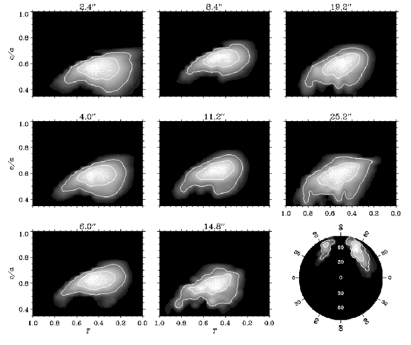
Figure 4: Intrinsic shape profile and orientation of NGC 4365, based on the “maximal ignorance” unweighted average of all models and a flat parent shape distribution. Rectangular panels show probability densities, in the space of triaxiality $T$ and short-to-long axis ratio $c/a$, for each radial zone; radii are indicated above each panel. Round figure at lower right shows probability density for the line of sight over a hemisphere, in Lambert equal-area polar projection; centre, right and left edges, and top and bottom edges of the figure correspond to views down the short, middle, and long axes of the galaxy, respectively. The direction of the angular momentum vector corresponds to a point along the upper half of a vertical line through the centre. The greyscale is logarithmic in all panels, and white contours enclose 68% and 95% of the total probability.

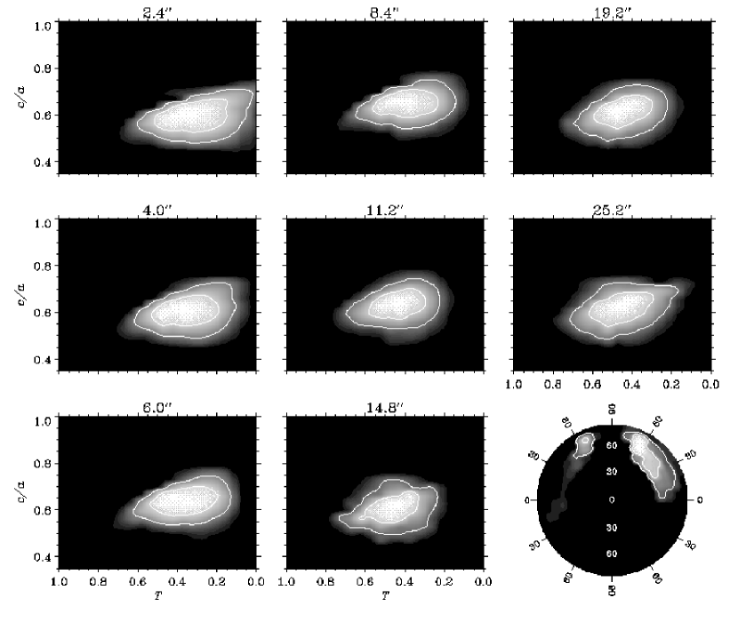
Figure 5: Same as Fig. 4, but using the parent shape distribution from Bak & Statler (2000).

In practice, the procedure is slightly complicated by technicalities needed to handle the 42-dimensional parameter space. The likelihoods for each radial bin are stored on a $20\times 20$ grid in triaxiality $T$ and axis ratio $c/a$, and an angular grid with approximately square bins of $\sim 10\mbox{${}^{\circ}$}$ resolution. The contribution to the likelihood from the VF and ellipticity data can be calculated independently at each radius, reducing storage demands considerably. We find it desirable at this stage to introduce a penalty for configurations that require unrealistically high internal velocities because the line of sight is close to the rotation axis (see the Appendix for a full explanation). Turning the likelihoods into the shape profile of the galaxy formally involves the construction of a joint distribution in 16 variables. To make this more manageable, we compute the projections of this distribution into each of the shape planes, and use these “marginal distributions” as the basic description of the shape profile. The procedure for combining the likelihood fits at each radius and including the isophotal PA data is explained in detail in the Appendix of Statler et al. (1999).

Construction of the prior involves a few subtle points which are described in detail in the Appendix of this paper. In brief, the prior distribution is assumed to separate into four factors:

$$F_{\rm prior} = {1\over 4\pi}F_{\rm par}[T_{i},(c/a)_{i}]F_{\rm cor}[T_{i}-T_{j},(c/a)_{i}-(c/a)_{j}]$$ (2)

$$\times F_{\rm int}[C_{i},k_{Xi},k_{Zi};T_{i},(c/a)_{i}].$$

The leading factor is the angular part, which we take to be isotropic over the viewing sphere. The second is the parent shape distribution; in principle this is a model for the shape distribution of all ellipticals, although for modeling a single system it is arguably better to use a flat distribution. We will show results for both a flat distribution and for the parent distribution derived from published long-slit data (Bak & Statler, 2000). The third part describes correlations in the joint shape distribution among the radial bins. These correlations reflect the fact that we expect the intrinsic shape to change continuously with radius. The last factor describes the distribution of the internal parameters, $C$, $k_{X}$, and $k_{Z}$. In the “maximal ignorance” estimate we assume no correlations of kinematics with radius. In other words, we explicitly allow for the possibility that there can be kinematically different populations dominating at different radii, bu we make no attempt to distinguish these populations, beyond their effects on the local mean streaming motions. In our standard model grid we also include a subset of models in which $C$ is correlated with shape at each radius, but these models give results consistent with the others.

3 Results

3.1 Intrinsic Shape Profile

The basic results are shown in Figure 4. The rectangular panels show the posterior probability distributions for the shape of the isodensity surfaces in the eight radial bins, based on an unweighted average of all computed models. Each panel depicts the $(T,c/a)$ plane and is plotted so that oblate spheroids ($T=0$) lie along the right edge and prolate spheroids ($T=1$) lie along the left edge. Spheres occupy the entire top margin at $c/a=1$, and the bottom margin, at $c/a=0.35$, corresponds to the observed upper limit on E galaxy ellipticities. The white curves indicate the 68% and 95% highest posterior density (HPD) regions, i.e., the contours enclosing 68% and 95% of the total probability, and may be thought of as $1\sigma$ and $2\sigma$ error regions.

It is clear that NGC 4365 is an almost maximally triaxial system. The preferred triaxialities are in the vicinity of $T\approx 0.4$–$0.5$, and axisymmetric and near-axisymmetric shapes are strongly ruled out, except perhaps in the innermost bin. There is an indication of an outward triaxiality gradient. The galaxy is also quite a bit flatter than it appears; photometry alone requires only that $c/a\loa 0.75$.

The results in Figure 4 are for a flat prior shape distribution, which is appropriate for one system modeled in isolation. But this part of the prior actually represents the parent shape distribution for the full population of ellipticals, which can be estimated from published long-slit kinematics. Bak & Statler (2000) model the Davies & Birkinshaw (1988) sample of 13 ellipticals, using methods very close to those of this paper, and derive several different parent distributions based on different assumptions for the dynamical prior. Their “maximal ignorance” result (their Fig. 2a) corresponds most closely to the dynamical prior used here. This distribution has broad peaks centred on the oblate and prolate limits, approximately at $(T,c/a)=(0,0.68)$ and $(1,0.82)$, with a broad ridge between them. Spheres and very flat, prolate-triaxial shapes have very low amplitude.

The shape profile of NGC 4365 using the Bak & Statler (2000) parent distribution is shown in Figure 5. The results are similar to those using the flat parent distribution, differing primarily in that the extended tail toward large $T$ and small $c/a$ is lacking. It is worth noticing that the single-galaxy shape constraint is improved when information from other objects is included in the form of the parent distribution. One can expect that the greatly superior parent distribution that will be derivable from the SAURON sample will permit even more precise single-galaxy shapes to be determined.

Figure 6: Radial triaxiality profiles derived from Figures 4 and 5 for the flat and Bak & Statler (2000) parent distributions. Points with error bars show expectation values and 68% HPD intervals ($1\sigma$ error bars); horizontal bars indicate the widths of the bins. Solid lines below denote 99%-confidence lower limits on $T$.

One dimensional triaxiality profiles can be straightforwardly calculated by integrating the distributions in Figures 4 and 5 over $c/a$. The results are shown in Figure 6. Error bars show the 68% HPD intervals, which are nearly centred on the expectation values. The systematic effect of changing the parent shape distribution is smaller than the statistical errors. There is an indication of a weak triaxiality gradient, but constant $T$ cannot be excluded. Possibly of greater interest for constraining the effects of chaos are lower limits on $T$; the continuous curves in the figure show 99%-confidence limits, which are significantly non-zero except possibly in the innermost bin.

3.2 Orientation

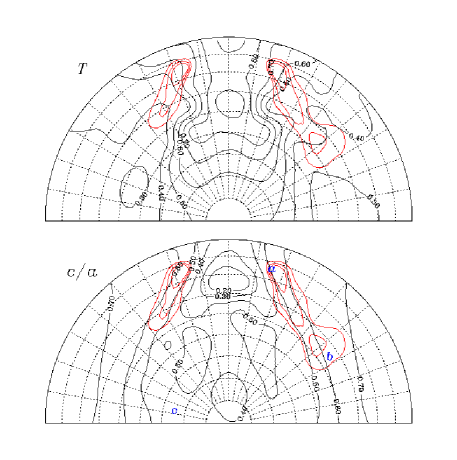
Figure 7: Lambert equal-area projections of half of the viewing hemisphere, showing (top) $T$ and (bottom) $c/a$ values of the best-fitting optimized model at each orientation (black contours). Overplotted in red are contours of $\Delta\chi_{\rm pen}^{2}$, at levels of $2.3$, $6.17$, and $11.8$. Models outside the outermost red contour are formally excluded at $>99\%$ confidence. Dotted lines show an angular grid at $10\mbox{${}^{\circ}$}$ spacing for reference. Letters in the lower panel indicate the 3 models shown in detail in Fig. 8.

The round panels in the lower right of Figures 4 and 5 show the posterior distributions for the line of sight, over one hemisphere. These are the orthogonal projections of the full posterior probability, integrated over shape, in contrast to the shape distributions which are integrated over orientation.

The line of sight is constrained to two fairly narrow strips, in the quadrant containing the angular momentum vector. That is, the true rotation axis in the outer part of the galaxy is most likely pointing in the general direction of the observer, as opposed to lying in the plane of the sky. Lines of sight $\sim 30\mbox{${}^{\circ}$}$ from the long axis are preferred, and those near the short axis are strongly excluded. These constraints are only slightly affected by the choice of the parent shape distribution.

The two strips in the orientation figures correspond to views on opposite sides of the $(x,z)$ plane, producing the same velocity field. Mirror-image points on the left and right sides of the figure differ only photometrically: for a given triaxiality gradient the isophotes twist in the opposite direction. If there were no observed isophotal twist, the figure would be left-right symmetric. The small asymmetry in the figure reflects the small ($\sim 2\mbox{${}^{\circ}$}$) observed twist over the fitted region.

3.3 Goodness of Fit; $\Delta\chi^{2}$ Confidence Limits

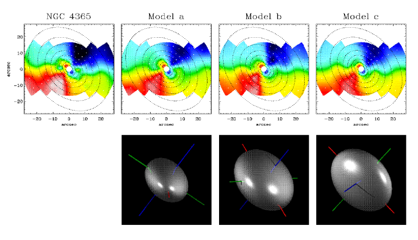
Figure 8: Data (top left) and models in the observational domain. Top row: isophotes and velocity fields, plotted as in Fig. 2. White points mark bin centres, where the fit is performed. Bottom row: ray-traced images of the mean shapes, as oriented in the sky. The shapes are rendered as polished metallic ellipsoids, symmetrically illuminated by lights to the right and left behind the observer. Red, green, and blue rods indicate the long, middle, and short axes. Models $a$, $b$, $c$ correspond to those indicated in Fig. 7, with ($a$) good, ($b$) marginal, and ($c$) poor fits.

A disadvantage of the Bayesian approach is that a posterior probability can be calculated even if the fit to the data is poor. It is therefore necessary to check separately that the best models are actually adequate fits in a $\chi^{2}$ sense. We couple our modeling code to a standard multidimensional optimizer and calculate, for each angular bin centre, the combination of shape and dynamical parameters that minimizes $\chi^{2}$ at that orientation. This allows us also to verify whether the HPD regions agree with confidence limits determined from $\chi^{2}$ contours.

We have 81 data points (66 velocities, 8 ellipticities, and 7 PA differences), and, at fixed orientation, 40 parameters ($T$, $c/a$, $C$, $k_{X}$, and $k_{z}$ in each radial bin). We minimize a $\chi^{2}$ statistic that includes the same penalties (for shape differences between adjacent bins and large internal $v/\sigma$) that are used in the Bayesian treatment. This adds 15 constraints, making $\nu_{\rm pen}=56$ degrees of freedom. The best optimized model has $\chi_{\rm pen}^{2}/\nu=1.14$. This is an acceptable fit; the probability of a larger $\chi_{\rm pen}^{2}$ occurring by chance is $0.22$. We also calculate, but do not optimize, the unpenalized $\chi_{\rm un}^{2}$ measuring only the fit to the data. The model optimized on $\chi_{\rm pen}^{2}$ has $\chi_{\rm un}^{2}/\nu_{\rm un}=1.41$, indicating an adequate but not spectacular fit.

In Figure 7 we plot in black the mean shape (unweighted average over the 8 radial bins) of the best optimized model at each orientation, for the half of the viewing hemisphere containing the viable models. These contours indicate only the best model for each line of sight, not whether these models are statistically good fits. Overplotted in red are contours of $\Delta\chi_{\rm pen}^{2}$, at levels of $2.3$, $6.17$, and $11.8$ above the minimum. Formally these correspond to 68%, 95%, and $99.7\%$ confidence intervals for two degrees of freedom, so lines of sight outside the last red contour are strongly ruled out. The models inside the red contours, which are not ruled out, have triaxialities $T$ between $0.32$ and $0.72$, and flattenings $c/a$ between $0.40$ and $0.68$. This is consistent with the results in Figure 4, which include many more models than just the best ones on each line of sight. Furthermore, the correspondence between the red $\Delta\chi_{\rm pen}^{2}$ contours in Figure 7 and the HPD contours in the bottom right of Figure 4 is qualitatively good; they clearly identify the same preferred lines of sight. The agreement is not exact, however. We attribute this to the difference between $\Delta\chi^{2}$ values computed, on the one hand, along an optimised $\chi^{2}$ valley floor in the space of the non-orientation parameters and, on the other, averaged over the whole valley at quite coarse resolution.

Notice that, on the viewing hemisphere, the $\chi^{2}$ valley is nearly parallel to the contours of optimized $c/a$, but cuts across the contours of optimized $T$. The fact that triaxialities $\sim 0.45$ are optimal over the broadest range of orientations is consistent with those values of $T$ being most probable (Figs. 4, 5, and 6). One should not place too much emphasis on the exact position of the $\chi^{2}$ minimum. Visual inspection of the acceptable models shows that different models fit different parts of the data better than others, and an alternative rebinning of the VF might easily have moved the $\chi^{2}$ minimum by $\sim 10\mbox{${}^{\circ}$}$ along the valley.

The blue letters in Figure 7 identify three representative models which we show in detail in Figure 8. Models $a$, $b$, and $c$ correspond to good, marginal, and bad fits respectively, having $\chi_{\rm un}^{2}/\nu$ values of $1.4$, $1.7$, and $2.8$, and $\chi_{\rm pen}^{2}/\nu$ values of $1.1$, $1.3$, and $2.3$. The top row of Figure 8 shows the projected isophotes and velocity field of each model, with the observed data from Figure 2b reproduced at top left. The bottom row shows a rendered-surface representation of an ellipsoid with the mean shape of each model, at the correct orientation. Clearly the acceptable models are able to reproduce the detailed kinematic and photometric structure of the galaxy. One can see from the figure that the biggest difficulty is simultaneously fitting the rotation amplitude and the steep velocity gradient near PAs $100\mbox{${}^{\circ}$}$ and $280\mbox{${}^{\circ}$}$. The unacceptable model $c$ does a particularly poor job of reproducing this gradient, and its kinematically distinct core region is too small.

3.4 Orbital Structure

Because we have allowed the orbit populations, by way of the velocity boundary condition, to vary freely with radius, the inferred shape profile and orientation of the system are essentially free of any assumptions about dynamical subsystems in the galaxy or its formation history. But, by the same token, we are unable to constrain the details of the stellar populations with these coarse models. That would be a job for much more sophisticated modeling, making use, at least, of the full line-of-sight velocity distributions, and possibly line-strength indices as well. None the less, we can draw some conclusions concerning what orbits dominate the net streaming motions in the inner and outer parts of the galaxy.

Figure 9: Intrinsic axis ratios of merger remnants and dark haloes from the literature. Each panel shows mean shapes or local shapes near the half-mass radius, as reported by the authors. Left: spiral-spiral merger remnants, without (Hernquist 1992, 1993, Barnes 1992) and with (Barnes & Hernquist 1996) gas dissipation. Center: Remnants of dissipationless group mergers (Weil & Hernquist 1996 as reanalysed by Statler et al. 2001, Zhang et al. 2002). Right: Distribution of zero-redshift halo shapes in a dissipationless $\Lambda$CDM cosmological simulation (Jing & Suto 2002) (contours; spaced by factor of 2 in density) and individual shapes of luminous objects in dissipational simulations (Sugarman et al. 2000, Meza et al. 2003).

To explore the dynamics of the kinematically distinct core, we compare three subsets of models in which the innermost zone is restricted to certain values of the contrast $C$: a Z-tube dominated configuration ($C=\infty,2$), an X-tube dominated configuration ($C=0,0.0625$), and a neutral configuration ($C=0.25,0.5$) We compute the maximum of the joint likelihood $L(T,c/a,\phi,\theta)$ in each radial bin, integrated over dynamical parameters but not over orientation. We find the Z-dominated configuration to have the highest peak likelihoods, with those in the neutral and X-dominated configurations smaller by factors of 5 and $3\times 10^{4}$, respectively. Insisting that the core rotation is entirely due to Z-tubes barely alters the shape profile. Axisymmetry in the core is still excluded at a $>2\sigma$ level. Photometrically, the isophotes between $1\arcsec$ and $3\arcsec$ are slightly discy (Carollo et al., 1997; Rest et al., 2001), and the large $h_{3}$ values in the same region are suggestive of discy kinematics. But a stellar disc embedded in a larger triaxial system will not, in general, be axisymmetric.

We can also investigate the dynamics of the region outside the core, by following the same procedure and restricting $C$ in the outer 4 zones. Here we find the situation reversed: the X-dominated configuration has the largest peak likelihoods, with the neutral and Z-dominated configurations down by factors of 4 and $10^{6}$, respectively.

We conclude, therefore, that the mean motions are most likely dominated by long-axis tubes in the main body of the galaxy and by short-axis tubes in the kinematically distinct core; this is essentially the configuration advocated by Surma & Bender (1995) for NGC 4365, and by Franx et al. (1991) for the similar system NGC 4406. It is virtually certain that the main body is not short-axis tube dominated, and that the core is not long-axis tube dominated. But configurations in which both tube families contribute significantly all through the galaxy cannot be ruled out. In fact, all of the models in Figure 8 require Z tubes in the main body to move the apparent rotation axis away from the position angle of the projected long axis.

4 Discussion

4.1 The Importance of Quantitative Measurements of Galaxy Shape

The distribution of three-dimensional shapes is an under-utilized, but potentially powerful diagnostic of galaxy formation physics. Numerical simulations of structure formation and galaxy mergers can now predict the axis ratios of the zero-redshift haloes or final merger remnants, and the results depend on the processes involved. Figure 9 shows representative results from the literature. Pair mergers of pure discs produce very flat, very triaxial remnants (Hernquist, 1992). Including dense bulges or moderate gas dissipation tends to make the final systems rounder and less prolate (Barnes, 1992; Hernquist, 1993; Barnes & Hernquist, 1996), in the former case because the merging systems are themselves rounder, and in the latter because of the scattering of low angular momentum orbits by the central mass accumulation. Significant dissipation in gas-rich mergers can flatten the final system if the gas settles into a disk and subsequently forms stars (Hernquist & Barnes, 1991; Barnes, 2002; Lamb & Hearn, 2003). Pure dark matter haloes formed in cosmological simulations are also very flat and prolate (Jing & Sato, 2002); as in disc mergers, including some dissipation tends to make the final systems rounder, though still strongly triaxial (Sugarman et al., 2000; Meza et al., 2003). Most prominently, mergers of groups should produce highly prolate or oblate remnants, depending on whether the initial system is collapsing or virialized (Weil & Hernquist, 1996; Garijo et al., 1997; Zhang et al., 2002). Clearly there is discriminating power in the shape distribution.

The SAURON instrument has produced stellar kinematic maps for two dozen elliptical galaxies (Emsellem et al.,, 2004). This paper constitutes the first step in using these data to determine the shape distribution. The results of the preceding section illustrate the power of two-dimensional data to constrain the shapes of individual systems. The axis ratios of NGC 4365 are determined to within approximately $0.1$, at the $1\sigma$ level. We have also modeled the SAURON VF for NGC 3379, and find that we can constrain the shape to comparable precision. The NGC 3379 results are very similar to those obtained from 7 long-slit profiles by Statler (2001). This is not surprising, since the VF is very simple and symmetric, and the SAURON map does not contain much additional information beyond what could be interpolated from the long-slit data. One may justifiably anticipate that it will be possible to determine the shapes and orientations of other objects in the SAURON sample to comparable precision using these methods, to estimate the parent shape distribution for the sample with the approach of Bak & Statler (2000), and to study the dependence of this distribution on galaxy luminosity or environment. These topics will be the focus of future papers.

4.2 Effects of Chaos; Limits on Central Black Hole Mass

NGC 4365 is an old system. From the metal and Balmer line indices Davies et al. (2001) infer an age $\goa 12\mbox{$\rm\,Gyr$}$ for the bulk of the stellar population, with at most a few percent admixture of a younger ($5\mbox{$\rm\,Gyr$}$) population in the centre. Absolute stellar ages are uncertain, however, and recent photometric (Puzia et al., 2002) and spectroscopic (Larsen et al., 2003) studies of globular clusters indicate the presence of an intermediate-age population. A minor merger $2$–$5\mbox{$\rm\,Gyr$}$ ago is not unlikely, although a significant event would probably have left photometric traces at large radii, which are not seen (Davies et al., 2001).

None the less, any age in the range of several Gyr implies that the system is dynamically very old. We can define a local relative dynamical age $\tau_{d}(r)$ as the ratio of the assembly age $t_{\star}$ to the crossing time at projected radius $r$. We approximate the latter as $r/[v_{m}^{2}(r)+\sigma^{2}(r)]^{1/2}$, where $v_{m}(r)$ is the maximum mean velocity at $r$. The result can be represented extremely well by the relation

$$\tau_{d}\approx 3\times 10^{4}\left({t_{\star}\over 10\mbox{$\rm\,Gyr$}}\right)\left({r\over 1\arcsec}\right)^{-1.1};$$ (3)

thus the entire SAURON field is hundreds of dynamical times old even if the galaxy was assembled as recently as $2\mbox{$\rm\,Gyr$}$ ago.

The long-term survival of triaxiality in systems with central density cusps or black holes has been questioned many times (Lake & Norman, 1983; Gerhard & Binney, 1985; Merritt, 1999, and references therein). Central mass concentrations can render a significant fraction of the box orbit phase space chaotic. Since box orbits are essential for maintaining triaxiality, it is believed that growth of a cusp or black hole can force a triaxial system to evolve toward axisymmetry or sphericity. That this has clearly not happened in NGC 4365 allows us to limit the maximum mass of a central black hole.

Calculating a precise upper limit is not yet possible. Surprisingly few numerical studies of chaos-driven morphological evolution have been performed, and these are not entirely appropriate to the properties of NGC 4365. Merritt & Quinlan (1998) start with a prolate-triaxial ($T\approx 0.6$, $c/a\approx 0.5$) equilibrium system with a flat, constant-density core, and grow central dark masses amounting to $0.3\%$, $1\%$, and $3\%$ of the galaxy mass. They see a large, rapid decrease in $T$ that effectively axisymmetrizes the entire system for mass ratios $\geq 1\%$. Below this mass the change is less drastic, but still pronounced. They also find that the shape evolution continues even after the central object reaches its final mass. Sellwood (2002) argues that this late evolution is a numerical artefact, but confirms Merritt & Quinlan’s basic result that mass ratios larger than 1% globally destroy triaxiality. Holley-Bockelmann et al. (2002) perform a similar experiment in which a 1%-mass black hole is grown in a somewhat rounder ($T=0.54$, $c=0.70$) triaxial system with an initial $r^{-1}$ density cusp. Unlike the flat-core systems, the cuspy system does not experience a global destruction of triaxiality. Its inner regions tend toward a spherical shape at approximately constant $T$, while the outer half of the system remains flattened and triaxial. The black hole creates a spherical region around itself containing several times its own mass in stars. The interpretation of these simulations is further complicated by the existence of flattened triaxial equilibria containing both cusps and central masses. Poon & Merritt (2002) construct equilibrium models for triaxial ($T=c/a=0.5$) nuclei with $r^{-1}$ and $r^{-2}$ cusps by Schwarzschild’s method. They confirm using $N$-body simulations that the shapes, even down to radii enclosing only a few times the black hole mass, are stable for $\sim 10$ crossing times. It is not known whether they would persist over tens of thousands of crossing times, as NGC 4365 would require. For whatever reason, these equilibria seem not to be found by the simulations that begin with no black hole. Evidently they do not have strong basins of attraction around them when the central mass grows dynamically.

We accept the basic result from Merritt & Quinlan (1998), Holley-Bockelmann et al. (2002), and Sellwood (2002), that a black hole $>1\%$ of the system mass will drive a rapid evolution of a region whose size is a significant fraction of the effective radius toward either axisymmetry or sphericity. This can be decisively ruled out in NGC 4365. To estimate the system mass, we use the total $V$-band magnitude, $V_{T}^{0}=9.5$, given in the RC3 (de Vaucouleurs et al., 1991), a distance modulus of $31.55$ (Tonry et al., 2001), and a mass-to-light ratio $M/L_{V}=6$ obtained by fitting an isotropic oblate Jeans model to the full SAURON data set. This $M/L_{V}$ is consistent with the results of Gebhardt et al. (2003), who find a mean $M/L_{V}=5.3$ for 11 ellipticals, with a dispersion of $2.1$. We obtain $M=3.3\times 10^{11}\mbox{$\,M_{\odot}$}$ for NGC 4365. This implies that a black hole of mass $M_{\rm BH}>3\times 10^{9}\mbox{$\,M_{\odot}$}$ would either globally axisymmetrize the galaxy or at least render the inner $10^{10}\mbox{$\,M_{\odot}$}$ spherical. By integrating the $\gamma=0.13$ Nuker model fit to the surface brightness profile (Rest et al., 2001), we find that this mass is enclosed in projection by the isophote with a mean radius of $3\arcsec$. Although we see indications of declining triaxiality at these radii, there is no significant rounding of the isophotes, which would be seen if the inner regions were becoming spherical. We conclude that the long-lived triaxiality in NGC 4365 rules out black holes of $M_{\rm BH}>3\times 10^{9}\mbox{$\,M_{\odot}$}$.

There is, as yet, no direct evidence for a black hole in NGC 4365. But for a mean dispersion of $260\mbox{${\rm\,km\,s}^{-1}$}$, the $M_{\rm BH}$-$\sigma$ relation (Gebhardt et al., 2000; Ferrarese & Merritt, 2000; Tremaine et al., 2002) would predict $M_{\rm BH}\approx 4\times 10^{8}\mbox{$\,M_{\odot}$}$. This corresponds to $\sim 0.1\%$ of the system mass, and probably would not drive a global shape change. If the single simulation of Holley-Bockelmann et al. (2002) can be extrapolated to lower masses, then a black hole of this mass might be expected to affect the isophotes in the inner $0\aas@@fstack{\prime\prime}9$. In the simulation, an $r^{-2}$ density cusp grows within the classical radius of influence of the black hole, which, for NGC 4365’s central dispersion of $270\mbox{${\rm\,km\,s}^{-1}$}$, would subtend $0\aas@@fstack{\prime\prime}1$. HST/WFPC2 surface photometry (Rest et al., 2001; Carollo et al., 1997) does show a gradual rounding of the isophotes interior to $1\arcsec$, reaching a minimum ellipticity $\sim 0.08$ at about $0\aas@@fstack{\prime\prime}16$. The central photometric structure is complicated, and may be affected by dust. There is no steepening of the $R$-band brightness profile within $0.1\arcsec$, but there does seem to be a central, unresolved source that is slightly ($\sim 0.02$ mag) bluer than its surroundings (Carollo et al., 1997).

Thus, while the persistent triaxiality of NGC 4365 excludes large black holes, a more modest object, on the scale predicted by the $M_{\rm BH}$-$\sigma$ relation, is probably small enough not to globally alter the shape of the galaxy and can be consistent with the data.

4.3 Figure Rotation

We have shown in § 3.4 that net streaming motions in long-axis tubes contributes significantly to, and probably dominates, the observed velocity field. The direct and retrograde branches of these orbits generate the same spatial density distribution if there is no rotation of the potential. However, if the galaxy is tumbling about the short axis, these orbits acquire a tilt with respect to the symmetry plane. This tilt increases for larger orbits, and is in the opposite direction for two senses of circulation. Since there must be an imbalance in the populations of the direct and retrograde branches, figure rotation would induce an intrinsic twist in the galaxy (Schwarzschild, 1982). The small observed photometric twist allows us to limit the tumbling rate.

The tilt of the periodic planar orbits out of the $(y,z)$ plane caused by figure rotation about the $z$ axis was examined by van Albada et al. (1982) and Heisler et al. (1982). These so-called “anomalous” orbits are the parents of the long-axis tubes (Schwarzschild, 1982), which we will assume acquire roughly the same tilt as the parent of the same energy. This assumption is by no means firmly established; the behavior of general orbits in tumbling figures has been studied only superficially (Salow 1998, unpublished). van Albada et al. (1982) show that the tilt angle $\alpha$ can be approximated by

$$\tan\alpha={2\over 1-(k/\omega)^{2}+(\Omega/\omega)^{2}}\cdot{\Omega\over\omega},$$ (4)

where $\omega$ and $k$ are the frequencies of the periodic motion in the plane and of oscillations out of the plane, respectively, in the absence of figure rotation, and $\Omega$ is the tumbling frequency. For slow tumbling, $\Omega$ can be ignored in the first factor. The ratio $k/\omega$ is a function of the axis ratios, and should be smaller than 1 for orbits around the long axis. For a triaxial modified Hubble model with $T=0.8$ and $c/a=0.5$, van Albada et al. (1982) calculate $k/\omega\approx 0.65$. Our models for NGC 4365 suggest shapes not quite as extreme as this. Let us suppose that $k/\omega\approx 0.8$, which is appropriate for a prolate logarithmic potential with a density axis ratio of roughly $0.6$. For NGC 4365 we approximate $\omega$ by $2^{1/2}\sigma/r$, with $\sigma\approx 220\mbox{${\rm\,km\,s}^{-1}$}$ the one-dimensional dispersion at $R\approx 20\arcsec$, and find that

$$\alpha\approx 0.4\mbox{${}^{\circ}$}\left({P_{\Omega}\over 1\mbox{$\rm\,Gyr$}}\right)^{-1}\left({r\over 1\arcsec}\right),$$ (5)

where $P_{\Omega}=2\pi/\Omega$ is the tumbling period.

It is interesting that the tilt is predicted to be linear in $r$. NGC 4365, in fact, has a linear isophotal twist of $0.09\mbox{${}^{\circ}$}/\arcsec$ for $2\arcsec<R<60\arcsec$. How the anomalous orbit tilt translates into an observed isophotal twist is extremely complicated, depending on the exact orbit populations, axis ratios, and viewing geometry, and is beyond our ability to predict in detail. However, if we imagine that the observed twist and the anomalous orbit tilt are of the same order of magnitude, then the observed twist could be caused by figure rotation if the tumbling period $P_{\Omega}\sim 5\mbox{$\rm\,Gyr$}$. Alternatively, we can say that $P_{\Omega}\loa 500\mbox{$\rm\,Myr$}$ is probably ruled out by the absence of a larger twist. This tumbling rate would place corotation at about 8 effective radii assuming a standard isothermal dark halo. It seems, therefore, safe to conclude that figure rotation is dynamically unimportant in the observable part of the galaxy.

If the isophotal twist is indeed due to figure rotation, then it is worth asking in what direction the figure is rotating. van Albada et al. (1982) performed this exercise for Centaurus A, in an effort to explain the warp of the dust lane. They predicted that the southwest side of the figure should be approaching and the northwest receding; unfortunately this was later found to be opposite to the sense of rotation of the stars. For NGC 4365, the required sense of figure rotation is northeast approaching and southwest receding for models viewed as in Figure 8a and 8b. Short-axis tubes are needed in these models, to displace the zero-velocity contour counter-clockwise on the sky. The sense of rotation of the short-axis tubes is therefore in the same direction as the figure tumbling, but opposite to the orbits of the same family that dominate the decoupled core.

4.4 Implications for Other Modeling Approaches

Although the VF fitting method can constrain the axis ratios and the orientation of the mass distribution, it does not make use of all of the available kinematic data, and consequently cannot truly constrain the full density profile. To do this, more sophisticated approaches are needed.

Jeans models have a long and distinguished history in galaxy dynamics. These models are built on the Jeans equations (Jeans, 1919; Chandrasekhar, 1960; Binney & Tremaine, 1987), which relate the second moments of the velocity distribution to the density distribution and the potential. Second-moment models are intuitively appealing, since luminous ellipticals are supported by velocity anisotropy (Binney, 1978). But fully anisotropic models are not easily computed because, in general, there are more independent second moments than there are Jeans equations to constrain them. Very recently, an analytic solution to the triaxial anisotropic Jeans equations has been demonstrated for systems with Stäckel potentials (van den Ven et al., 2003). It may be possible to use this result to create simple, approximate second-moment models, and to merge the VF fitting and Jeans techniques (van de Ven et al., in preparation).

A full understanding of the dynamical structure of a galaxy requires a model for the complete phase space distribution function. At present the only workable technique to build such a model is Schwarzschild’s method (Schwarzschild, 1979). In this technique a finite library of test-particle orbits is populated to reproduce a desired mass distribution and fit the photometric and kinematic data. The newest Schwarzschild code for triaxial systems is presented by Verolme (2003) and Verolme et al. (2004); but unfortunately, no direct comparison of Schwarzschild and VF fitting results for NGC 4365 is yet possible. Schwarzschild models, by allowing any population of stars on any orbit, have far more freedom than the continuity-equation models used in VF fitting. We suspect that a Schwarzschild code may be able to find models that fit the data outside our statistically allowed region. But we also suspect that these models may be very unsmooth in phase space. How a physical requirement of smoothness is best imposed on Schwarzschild models is a matter of vigorous debate (Valluri et al., 2004).

The SAURON kinematic maps constitute the best data to date for revealing the dynamical structure of elliptical galaxies. To fully realize the potential of these data will require the application of a variety of modeling approaches, including Schwarzschild’s method, Jeans models, and VF fitting. But it is not feasible to apply the most computationally expensive method blindly; each approach should be informed by the results of coarser methods that can survey more territory. This paper provides an initial rough map of the parameter space for NGC 4365, as a guide for more detailed modeling efforts to follow.

5 Summary

We have modeled the two-dimensional mean velocity field and isophotal profiles of the old and kinematically interesting elliptical galaxy NGC 4365 using the VF fitting approach, and constrained the system’s intrinsic shape between $0.03$ and $0.5$ effective radii and its orientation in space. We find that the galaxy is highly triaxial ($\langle T\rangle\approx 0.45$) and somewhat flatter than it appears ($\langle c/a\rangle\approx 0.6$). Axisymmetry or near axisymmetry ($T<0.1$) is ruled out at better than 95% confidence everywhere, and at better than 99% confidence everywhere except in the inner $3\arcsec$. There is a weak indication of an outward triaxiality gradient. The orientation of the galaxy is constrained to two fairly narrow strips on the viewing hemisphere. In the most probable models the system is oriented with its long axis pointing in the general direction of the observer, extending in projection to the southwest. We have verified that the best models are statistically acceptable in a $\chi^{2}$ sense, and that $\Delta\chi^{2}$ regions and Bayesian HPD regions define essentially the same region of permitted parameter space.

That strong triaxiality has evidently persisted in the galaxy for some $12\mbox{$\rm\,Gyr$}$ implies that any central black hole must be smaller than $3\times 10^{9}\mbox{$\,M_{\odot}$}$. A larger central mass would have induced chaos sufficient either to globally axisymmetrize the galaxy or at least make the inner several arcseconds spherical. On the other hand, a black hole of mass $4\times 10^{8}\mbox{$\,M_{\odot}$}$, as predicted by the $M_{\rm BH}$-$\sigma$ relation, would probably not preclude long-lived triaxiality and is consistent with the observations.

We find that there must be a significant contribution from long-axis tubes outside the kinematically decoupled core, and that the direct and retrograde branches of these orbits must be unequally populated so as to produce the observed rotation signature. This permits us to constrain the rate of figure rotation about the short axis, since figure rotation would induce an intrinsic twist. From the observed photometric twist we infer that the tumbling period is $\goa 500\mbox{$\rm\,Myr$}$, putting corotation at at least 8 effective radii, and supporting the common assumption that figure rotation is dynamically unimportant in luminous ellipticals.

NGC 4365 contributes to an emerging picture of the role of black holes in giant elliptical galaxies: though omnipresent, black holes are not massive enough to alter the global structure of their hosts, which can remain anisotropic and triaxial for many hundreds of dynamical times. It is still undetermined whether this same picture may apply to lower-luminosity systems, however, and it is possible that there is a threshold below which central black holes drive a secular evolution toward axisymmetry. The SAURON project has produced a rich database which will make it finally possible to address these and related issues. Determining the mass distributions and the dynamical structure of early-type galaxies will require extensive modeling using Schwarzschild’s method, as well as faster but more idealized moment-based methods such as we have used. We hope that through an application of such complementary approaches, it will be possible to develop a more complete understanding of the dynamical histories of hot stellar systems.

Appendix A Prior Distributions and Penalty Functions

The separation of the prior distribution into factors for the orientation, the parent mean shape distribution, shape correlations, and the dynamical parameter distribution is explained in § 2.3. This appendix describes the details of the last two factors.

A.1 Shape Prior

The prior shape distribution for 8 radial bins is a joint distribution in 16 variables. It may seem least biased to let this function be constant everywhere and allow any shape at each radius, but this is not the case. The shape parameter space at each radius is two-dimensional, and so a flat distribution implies that large differences in shape between adjacent radii are likely simply because there is more area in a plane far from a given point than close to it. If the observations show that the galaxy appears similar at neighboring radii—in particular, that the isophotal twist is small—then the Bayesian “robot” (Jaynes, 2003) is forced to reason as follows: neighboring radii probably have very different shapes, yet in projection they appear very similar; so we must be looking at the galaxy along one of the special lines of sight where big changes of shape are not noticeable. The results will then be biased toward lines of sight in the symmetry planes.

From observations of many ellipticals it is already known that radial photometric gradients tend to be small, and therefore that shape profiles are probably smooth and shapes at neighboring radii are correlated. Expected correlations must be included in the prior (Jaynes, 2003). We do this by imposing a Gaussian penalty factor of the form

$$F_{\rm cor}=\prod_{i=2}^{8}\exp\left\{-{(T_{i}-T_{i-1})^{2}+[(c/a)_{i}-(c/a)_{i-1}]^{2}\over 2\sigma_{g}^{2}}\right\},$$ (6)

which penalizes differences in $T$ and $c/a$ between neighboring radii (Statler, 2001, § 3.2.2). We set the constant $\sigma_{g}=0.126$, so as to render a complete change of shape, e.g., from $T=0$ to $T=1$ or $c/a=0$ to $c/a=1$ over the observed range of radii, a priori unlikely at the $3\sigma$ level. Other values of $\sigma_{g}$ in the range $0.1$ to $0.2$ give very similar results.

A.2 Dynamical Prior

The parent distribution of the dynamical parameters $C$, $k_{X}$, and $k_{Z}$ is defined by the grid of values over which we compute models. For the Z-tube/X-tube contrast we take $C=(0,0.0625,0.125,0.25,0.5,1.0,2.0,\infty)$. The limiting values $C=0$ and $C=\infty$ correspond to zero net streaming in Z-tubes and X-tubes, respectively. We also add four more cases, where $C$ is assumed to be a function of $T$ and $c/a$ according to each of the four “prescription” functions introduced in equations (11)–(14) of Statler (1994b). We find that the results from the regular grid alone are nearly indistinguishable from those including the prescriptions, indicating that explicit correlations between shape and dynamics are unimportant.

The other constants $k_{X}$ and $k_{Z}$ determine the “disc-like” or “spheroid-like” character of the mean streaming in each tube family. A lower value indicates more disc-like kinematics, meaning that the mean velocity decreases more rapidly away from the symmetry plane. We take $k_{X}=(0,0.25,0.5,0.75,1.0,1.25,1.5)$ and $k_{Z}=(0,0.25,0.5,0.75,1.0)$, based on the behavior of numerical and analytic self-consistent triaxial models [see Figure 8 of Statler (1994a)].

A.3 $v/\sigma$ Penalty

The magnitude of any velocity field can be scaled up or down by reversing the direction of some fraction of the stars on tube orbits. Accordingly, the model velocities are determined only to within a constant factor and then scaled to fit the data. In previous work we have allowed the scaling constant to vary freely. However, we find that this practice leads to biased results when the apparent rotation axis is far from a symmetry axis. The reason is that the fitting procedure can most easily produce a model with the apparent rotation axis along an arbitrary direction merely by placing the line of sight very close to the true rotation axis, and then slightly inclining the model in the right direction. But in this case the low $\sin i$ factor may imply deprojected internal velocities that are unrealistically large.

To avoid these unphysical models, we calculate for each projected model at each radius the maximum deprojected velocity on the shell, $v_{s}$, required by the optimal scaling, and then penalize the model by a factor $\exp(-v_{s}^{2}/2\sigma^{2})$. We take the parameter $\sigma$ to be the observed velocity dispersion at that radius, so in other words we are penalizing models with internal $v/\sigma$ values greater than 1. This turns out to be a fairly weak penalty in nearly all regions of parameter space, affecting lines of sight only within about $15\mbox{${}^{\circ}$}$ of the true rotation axis.

References

- Adams et al. (2003) Adams, F. C., Graff, D. S., Mbonye, M., & Richstone, D. O. 2003, ApJ, 591, 125
- Anderson & Statler (1998) Anderson, R. F. & Statler, T. S. 1998, ApJ, 496, 706
- Bacon et al. (2001) Bacon, R., Copin, Y., Monnet, G., Miller, B. W., Allington-Smith, J. R., Bureau, M., Carollo, C. M., Davies, R. L., Emsellem, E., Kuntschner, H., Peletier, R. F., Verolme, E. K., & de Zeeuw, P. T. 2001, MNRAS, 326, 23
- Bak & Statler (2000) Bak, J. and Statler, T. S. 2000, AJ, 120, 110
- Barnes (1992) Barnes, J. E. 1992, ApJ, 393, 484
- Barnes (2002) Barnes, J. E. 2002, MNRAS, 333, 481
- Barnes & Hernquist (1996) Barnes, J. E. & Hernquist, L. 1996, ApJ, 471, 115
- Bender et al. (1988) Bender, R., Döbereiner, S., & Möllenhoff, C. 1988, A&AS, 74, 385
- Binney (1978) Binney, J. 1985, MNRAS, 183, 501
- Binney (1985) Binney, J. 1985, MNRAS, 212, 767
- Binney & Tremaine (1987) Binney J. & Tremaine, S. 1987, Galactic Dynamics, Princeton University Press, Princeton, NJ
- Cappellari & Copin (2003) Cappellari, M. & Copin, Y. 2003, MNRAS, 342, 345
- Carollo et al. (1997) Carollo, C. M., Franx, M., Illingworth, G. D., & Forbes, D. A. 1997, ApJ, 481, 710
- Chandrasekhar (1960) Chandrasekhar, S. 1960, Principles of Stellar Dynamics, Dover, New York, NY
- Davies & Birkinshaw (1988) Davies, R. L. & Birkinshaw, M. 1988, ApJS, 68, 409
- Davies et al. (2001) Davies, R. L., Kuntschner, H., Emsellem, E., Bacon, R., Bureau, M., Carollo, C. M., Copin, Y., Miller, B. W., Monnet, G., Peletier, R. F., Verolme, E. K., & de Zeeuw, P. T. 2001, ApJ, 548, L33
- de Vaucouleurs et al. (1991) de Vaucouleurs, G., de Vaucouleurs, A., Corwin H. G., Jr., Buta, R. J., Paturel, G., & Fouque, P. 1991, Third Reference Catalogue of Bright Galaxies, Version 3.9.
- de Zeeuw et al. (2002) de Zeeuw, P. T., Bureau, M., Emsellem, E., Bacon, R.. Carollo, C. M., Copin, Y., Davies, R. L., Kuntschner, H., Miller, B. W., Monnet, G., Peletier, R. F., & Verolme, E. K. 2002, MNRAS, 329, 513
- Djorgovski & Davis (1987) Djorgovski, S. & Davis, M. 1987, ApJ, 313, 59
- Dressler et al. (1987) Dressler, A., Lynden-Bell, D., Burstein, D., Davies, R. L., Faber, S. M., Terelvich, R. J., & Wegner, G. 1987, ApJ,
- El Zant et al. (2003) El-Zant, A. A., Shlosman, I., Begelman, M. C., & Frank, J. 2003, ApJ, 590, 641
- Emsellem et al., (2004) Emsellem, E., Cappellari, M., Peletier, R., McDermid, R., Bacon, R., Bureau, M., Copin, Y., Davies, R. L., Krajnović, D., Kuntschner, H., Miller, B, & de Zeeuw, P. T. 2004, MNRAS, submitted
- Ferrarese & Merritt (2000) Ferrarese, L. & Merritt, D. 2000, ApJ, 539, L9
- Forbes (1994) Forbes, D. A. 1994, AJ, 107, 2017
- Franx et al. (1991) Franx, M., Illingworth, G., & Heckman, T. 1989, ApJ, 344, 613
- Franx et al. (1991) Franx, M., Illingworth, G., & de Zeeuw, T. 1991, ApJ, 383, 112
- Gebhardt et al. (2000) Gebhardt, K., Bender, R., Bower, G., Dressler, A., Faber, S. M., Filippenko, A. V., Green, R., Grillmair, C., Ho, L. C., Kormendy, J., Magorrian, J., Pinkney, J., Richstone, D., & Tremaine, S. 2000, ApJ, 539, L13
- Gebhardt et al. (2003) Gebhardt, K., Richstone, D., Tremaine, S., Lauer, T. R., Bender, R., Bower, G., Dressler, A., Faber, S. M., Filippenko, A. V., Green, R., Grillmair, C., Ho, L. C., Kormendy, J., Magorrian, J., & Pinkney, J. 2003, ApJ, 583, 92
- Garijo et al. (1997) Garijo, A., Athanassoula, E., & Garcia-Gomez, C. 1997, A&A, 327, 930
- Gerhard & Binney (1985) Gerhard, O. E. & Binney, J. 1985, MNRAS, 216, 467
- Gerhard (1986) Gerhard, O. E. 1986, MNRAS, 219, 373
- Hasan & Norman (1990) Hasan, H. & Norman, C. 1990, ApJ, 361, 69
- Hernquist (1992) Hernquist, L. 1992, ApJ, 400, 460
- Hernquist (1993) Hernquist, L. 1993, ApJ, 409, 548
- Hernquist & Barnes (1991) Hernquist, L. & Barnes, J. 1991, Nature, 354, 210
- Heisler et al. (1982) Heisler, J., Merritt, D., & Schwarzschild, M. 1982, ApJ, 258, 490
- Holley-Bockelmann et al. (2002) Holley-Bockelmann, K., Mihos, J. C., Sigurdsson, S., Hernquist, L., & Norman, C. 2002, ApJ, 567, 817
- Jaynes (2003) Jaynes, E. T. 2003, Probability Theory: The Logic of Science, Cambridge University Press, Cambridge
- Jeans (1919) Jeans, J. H. 1919, Phil. Trans. Roy. Soc. London A, 218, 157
- Jing & Sato (2002) Jing, Y. P. & Sato, Y. 2002, ApJ, 574, 538
- Lamb & Hearn (2003) Lamb, S. A. & Hearn, N. C. 2003, Ap&SS, 284, 479
- Lake & Norman (1983) Lake, G. & Norman, C. 1983, ApJ, 270, 51
- Larsen et al. (2003) Larsen, S. S., Brodie, J. P., Beasley, M. A., Forbes, D. A., Kissler-Patig, M., Kuntschner, H., & Puzia, T. H. 2003, ApJ, 585, 767
- Merritt (1996) Merritt, D. 1999, Science, 271, 337
- Merritt (1999) Merritt, D. 1999, PASP, 111, 247
- Merritt & Fridman (1996) Merritt, D. & Fridman, T. 1996, ApJ, 460, 136
- Merritt & Quinlan (1998) Merritt, D. & Quinlan, G. 1998, ApJ, 498, 625
- Meza et al. (2003) Meza, A., Navarro, J. F., Steinmetz, M., & Eke, V. R. 2003, ApJ, 590, 619
- Norman et al. (1996) Norman, C. A., Sellwood, J. A., & Hasan, H. 1996, ApJ, 462, 114
- Poon & Merritt (2001) Poon, M. Y. & Merritt, D. 2001, ApJ, 549, 192
- Poon & Merritt (2002) Poon, M. Y. & Merritt, D. 2002, ApJ, 568, L89
- Puzia et al. (2002) Puzia, T. H., Zepf, S. E., Kissler-Patig, M., Hilker, M., Minniti, D., & Goudfrooij, P. 2002, A&A, 391, 453
- Rest et al. (2001) Rest, A., van den Bosch, F. C., Jaffe, W., Tran, H., Tsvetanov, Z., Ford, H. C., Davies, J., & Schafer, J. 2001, AJ, 121, 2431
- Rix et al. (1997) Rix, H.-W., de Zeeuw, P. T., Cretton, N., van der Marel, R. P., Carollo, C. M. 1997, ApJ, 488, 702
- Schwarzschild (1979) Schwarzschild, M. 1979, ApJ, 232, 236
- Schwarzschild (1982) Schwarzschild, M. 1982, ApJ, 263, 599
- Schwarzschild (1993) Schwarzschild, M. 1993, ApJ, 409, 563
- Sellwood (2002) Sellwood, J. A. 2002, in The Shapes of Galaxies and their Dark Halos, ed P. Natarajan, World Scientific, Singapore, 123
- Siopis & Kandrup (2000) Siopis, C. & Kandrup, H. E. 2000, MNRAS, 319, 43
- Sridhar & Touma (1997) Sridhar, S. & Touma, S. 1997, MNRAS, 287, L1
- Sridhar & Touma (2000) Sridhar, S. & Touma, S. 2000, ApJ, 542, 143
- Statler (2001) Statler, T. S. 2001, AJ, 121, 244
- Statler (1994a) Statler, T. S. 1994a, ApJ, 425, 458
- Statler (1994b) Statler, T. S. 1994b, ApJ, 425, 500
- Statler et al. (1999) Statler, T. S., Dejonghe, H., & Smecker-Hane, T. 1999, AJ, 117, 126
- Statler et al. (1996) Statler, T. S., Smecker-Hane, T., & Cecil, G. 1996, AJ, 111, 1512
- Statler et al. (2001) Statler, T. S., Lambright, H., & Bak, J. 2001, ApJ, 549, 871
- Sugarman et al. (2000) Sugarman, B., Summers, F. J., & Kamionkowski, M. 2000, MNRAS, 311, 762
- Surma & Bender (1995) Surma, P. & Bender, R. 1995, A&A, 298, 405
- Tonry et al. (2001) Tonry, J. L., Dressler, A., Blakeslee, J. P., Ajhar, E. A., Fletcher, A. B., Luppino, G. A., Metzger, M. R., & Moore, C. B. 2001, ApJ, 546, 681
- Tremaine et al. (2002) Tremaine, S., Gebhardt, K., Bender, R., Bower, G., Dressler, A., Faber, S. M., Filippenko, A. V., Green, R., Grillmair, C., Ho, L. C., Kormendy, J., Magorrian, J., Pinkney, J., & Richstone, D. 2002, ApJ, 574, 740
- Valluri & Merritt (1998) Valluri, M. & Merritt, D. 1998, ApJ, 506, 596
- Valluri et al. (2004) Valluri, M., Merritt, D., & Emsellem, E. 2004, ApJ, 602, 66
- van Albada et al. (1982) van Albada, T. S., Kotanyi, C. G., & Schwarzschild, M. 1982, MNRAS, 198, 303
- van den Ven et al. (2003) van de Ven, G., Hunter, C., Verolme, E. K., & de Zeeuw, P. T. 2003, MNRAS, 342, 1056
- van der Marel & Franx (1993) van der Marel, R. P., & Franx, M. 1993, ApJ, 407, 525
- Verolme (2003) Verolme, E. K. 2003, Proefshrift, Univ. Leiden
- Verolme et al. (2004) Verolme, E. K., Cappellari, M., Emsellem, E., van de Ven, G., & de Zeeuw, P. T. 2004, MNRAS, submitted
- Weil & Hernquist (1996) Weil, M. & Hernquist, L. 1996, ApJ, 460, 101
- Zhang et al. (2002) Zhang, B., Wyse, R. F. G., Stiavelli, M., & Silk, J. 2002, MNRAS, 332, 647