Resonant Excitation of White Dwarf Oscillations in Compact Object Binaries: 1. The No Back Reaction Approximation

Abstract

We consider the evolution of white dwarfs with compact object companions (specifically black holes with masses up to $\sim 10^{6}$ M_⊙, neutron stars, and other white dwarfs). We suppose that the orbits are initially quite elliptical and then shrink and circularise under the action of gravitational radiation. During this evolution, the white dwarfs will pass through resonances when harmonics of the orbital frequency match the stellar oscillation eigenfrequencies. As a star passes through these resonances, the associated modes will be excited and can be driven to amplitudes that are so large that there is a back reaction on the orbit which, in turn, limits the growth of the modes. A formalism is presented for describing this dynamical interaction for a non-rotating star in the linear approximation when the orbit can be treated as non-relativistic. A semi-analytical expression is found for computing the resonant energy transfer as a function of stellar and orbital parameters for the regime where back reaction may be neglected. This is used to calculate the results of passage through a sequence of resonances for several hypothetical systems. It is found that the amplitude of the $\ell=m=2$ f-mode can be driven into the non-linear regime for appropriate initial conditions. We also discuss where the no back reaction approximation is expected to fail, and the qualitative effects of back reaction.

1 Introduction

White dwarfs, the normal evolutionary endpoint for stars less massive than $\sim 8$ M_⊙, are extremely common; the halo of our Galaxy contains several billion of them. They are observed frequently in binary systems, with normal stellar companions, as cataclysmic variable stars and, less often, with compact object companions, WDCO systems. Many of these systems are produced naturally in binary star evolution and, as a consequence, have circular orbits. However, it is also possible to form eccentric, WDCO binaries following stellar capture or exchange in a dense stellar environment. In the present paper, we do not consider the formation of such binaries in detail; we list some possible formation mechanisms, but our detailed considerations are restricted to the evolution of such systems after they form.

There are three possible types of WDCO systems. Perhaps the most common are double degenerates (e.g. Maxted et al., 2002), which have been observed to have periods as short as $\sim 5$ min (Ramsay et al., 2002). A second class is white dwarf-neutron star binaries, of which there are over 50 known or suspected (Lorimer, 2001), with orbital periods as short as 3 hr (Edwards & Bailes, 2000). The third class are white dwarf-black hole binaries. For black hole companions in the stellar mass range, there are no known examples–they would be extremely hard to find. There is, however, growing theoretical evidence for, and observational evidence consistent with, the existence of intermediate mass black holes (IMBHs). X-ray observations of nearby galaxies hint at the possibility of a large population of black holes in the $\sim 10^{2}$–$10^{4}$ M_⊙ mass range (Colbert & Mushotzky, 1999; Colbert & Ptak, 2002). The interpretation of these observations is the source of some debate, but accreting IMBHs are certainly a plausible explanation. These IMBHs may have been formed in the early universe from $10^{2}$–$10^{3}$ M_⊙ stars (Bromm et al., 1999). Also, recent dynamical simulations of dense stellar clusters have demonstrated that runaway collisions can lead rapidly to the formation of black holes with masses in the $\sim 10^{2}$–$10^{3}$ M_⊙ range (Portegies Zwart et al., 2004). More generally, the population of IMBHs could span the entire interval between stellar and massive black holes ($\sim 10^{2}$–$10^{6}$ M_⊙). They could either tidally capture white dwarfs from the field (Fabian et al., 1975; Press & Teukolsky, 1977), or participate in three-body processes in stellar clusters and end up in bound orbits with white dwarf companions (Hills, 1977).

The tidal capture mechanism is simple in principle. When the radius of periastron is no more than a few times the Roche limit, the normal modes of the white dwarf can be excited non-resonantly. On egress, the energy of the oscillation is taken out of the orbit, which can become bound. The energy transfer need be no more than $\sim$($30$–$100$ km s^-1)${}^{2}\equiv 10^{13-14}$ erg g${}^{-1}\equiv 10$–$100$ eV per nucleon for capture to ensue. Subsequent periastron passages can lead to additional mode excitation and the possibility of heating the star if the oscillation energy is thermalised. For a black hole companion, this mechanism requires that the Roche limit lie not too far inside the event horizon, which sets an upper limit of $\sim 10^{6}$ M_⊙ on the black hole mass. (When the black hole mass exceeds $\sim 3\times 10^{5}$ M_⊙, it turns out that gravitational bremsstrahlung is more important than tidal capture and contributes a larger capture cross-section.)

Whatever their detailed nature and origin, WDCO binaries evolve dynamically under the action of gravitational radiation. The orbital periods and eccentricities will decrease until the former reaches the Roche period, $\sim 10-100$ s depending upon mass, when the star will be torn apart by tidal forces. During inspiral, a WDCO system will pass through a series of resonances between harmonics of the orbital frequency and the white dwarf normal mode eigenfrequencies. Typically, the system will spend many orbits near each resonance, and consecutive resonances for a given mode will be separated by a much larger number of orbits associated with the gravitational inspiral time-scale. Passage through a sequence of such resonances will result in transfer of energy from the orbit to the oscillations and may drive the amplitudes of the oscillations non-linear, with possibly observable consequences.

If the energy transfer from the orbit to the stellar oscillation is as large as $\sim 10$ keV per nucleon and the mode energy is thermalised, then it is possible to detonate the star, releasing more nuclear energy ($\sim 1$ MeV per nucleon) than the gravitational binding energy ($\sim 0.1$–$0.3$ MeV per nucleon). Typically, for a black hole companion, the orbital binding energy will be greater than the nuclear energy released, so most of the ejecta will be trapped. However, for a white dwarf or neutron star companion, the ejecta can become unbound.

We note that WDCO binaries also constitute one of the prime potential sources for LISA (e.g. Finn & Thorne, 2000). The considerations presented below may be relevant to gravitational wave observations of these systems.

In order to understand how much energy is transferred from the orbit to the white dwarf during inspiral, it is necessary to consider the evolution of the system after it has lost much of its initial eccentricity. We present a general formalism for handling tidal resonances in WDCO binaries in the linear normal mode approximation. We restrict ourselves to non-rotating stars because white dwarfs are observed generally to be slowly rotating, and they are not expected to maintain corotation during inspiral (c.f. Bildsten & Cutler, 1992). However, this needs further investigation. In addition, we mostly confine our attention to the $\ell=m=2$ f-mode because it is expected to be the dominantly excited one. Nonetheless, our formalism may be applied to other modes as well. Of particular interest may be $g$-modes, as these have lower frequencies than the $f$-modes, and can therefore be excited at fundamental resonance in circular orbits before tidal disruption.

We begin with a description of the general formalism in §2. This includes a brief description of the resonant excitation of a simple harmonic oscillator (§2.1), a summary of the structure and normal modes of cold white dwarfs (§2.2), an overview of gravitational radiation reaction (§2.3), and our formalism for tidal excitation (§2.4). In §3, we discuss some physical aspects of the dynamical problem, including mode damping and time-scales. We also discuss the physical regimes where various effects are important. In §4, we apply the general formalism to calculate the energy transfer for a resonance in an eccentric orbit, ignoring back reaction. In §5, we discuss the regime where this result is expected to be valid, and describe the qualitative effects of back reaction. This is followed by a description of the long term evolution of WDCO binaries in the absence of back reaction. We present our conclusions in §6.

2 General Formalism

2.1 Simple harmonic oscillator

Consider an undamped simple harmonic oscillator with natural frequency $\omega_{0}$ and displacement $x(t)$ subject to an external force per unit mass $F(t)$. The equation of motion,

$$\ddot{x}+\omega_{0}^{2}x=F(t)\ ,$$ (1)

can be easily solved to get

$$\dot{x}(t) =\Re\left[\zeta(t)\right]\ ,$$ (2)

$$x(t) =\frac{1}{\omega_{0}}\Im\left[\zeta(t)\right]\ ,$$ (3)

where

$$\zeta(t)=\zeta_{0}e^{i\omega_{0}t}+\zeta_{1}(t)\ ,$$ (4)

and

$$\zeta_{1}(t)\equiv e^{i\omega_{0}t}\int_{t_{0}}^{t}dt^{\prime}\,e^{-i\omega_{0}t^{\prime}}F(t^{\prime})\ .$$ (5)

It follows from the expressions for $x$ and $\dot{x}$ in terms of $\zeta$ that the total energy per unit mass of the oscillator as a function of time is given by

$$E(t)=\frac{1}{2}\left|\zeta(t)\right|^{2}\ .$$ (6)

Let the external force per unit mass now be of the form

$$F(t)=F_{0}(t)\cos\left[\phi(t)\right]\ ,$$

with the amplitude $F_{0}$ and frequency $\dot{\phi}$ being slowly varying functions of time, and $\ddot{\phi}>0$. Resonance occurs when the relative phase of the driver and the oscillator becomes stationary. This gives us the condition $\dot{\phi}(t)=\omega_{0}$. We assume that there is only one passage through resonance, and since there will be little average energy transfer away from resonance, we need only consider the form of the forcing function near resonance. Let $t_{R}$ be the time when the resonance condition is satisfied, and expand the driver in a Taylor series around this point:

$$F(t_{R}+\tau)\simeq F_{0}(t_{R})\cos\left[\phi(t_{R})+\omega_{0}\tau+\ddot{\phi}(t_{R})\frac{\tau^{2}}{2}\right]\ .$$ (7)

(Since the amplitude varies slowly with time, to lowest order, we can take the amplitude as constant through the resonance.) With the definitions

$$F_{R}\equiv F_{0}(t_{R})\ ,\quad\phi_{R}\equiv\phi(t_{R})\ ,\quad\alpha\equiv\frac{\ddot{\phi}(t_{R})}{\omega_{0}^{2}}\ ,$$

this becomes

$$F(t_{R}+\tau)\simeq F_{R}\cos\left(\phi_{R}+\omega_{0}\tau+\alpha\frac{\omega_{0}^{2}\tau^{2}}{2}\right)\ .$$ (8)

The parameter $\alpha$ has the physical interpretation of being a measure of the fractional change in frequency over a characteristic period of oscillation. The requirement that the frequency of the driver is varying slowly therefore implies $\alpha\ll 1$. In other words, the driver can be considered harmonic with a well-defined frequency over several periods of the oscillator. We can also view $\alpha$ as a measure of the phase “drift”–i.e. a measure of how fast the driver accumulates additional phase. With this interpretation, it is easy to see that the time spent near resonance is given by $(\alpha\omega_{0}^{2})^{-1/2}$, approximately.

The problem of solving for the motion of the oscillator is now mathematically similar to the theory of Fresnel diffraction, and the solution can be expressed in terms of Fresnel integrals. We relegate the detailed calculation to Appendix A and simply summarise the result:

$$\begin{split}\zeta_{1}=\frac{F_{R}}{2}e^{i\omega_{0}\tau}\Bigg{\{}&I_{1}(\tau)\exp\left(i\phi_{R}\right)\\ &+I_{2}(\tau)\exp\left[-i\left(\phi_{R}-\frac{2}{\alpha}\right)\right]\Bigg{\}}\ ,\end{split}$$

where $I_{1}$ and $I_{2}$ are given by expressions involving Fresnel integrals. The time-averaged energy per unit mass changes asymptotically by

$$\Delta E=\frac{\pi F_{R}^{2}}{4\alpha\omega_{0}^{2}}\left(1+2\sqrt{\frac{E_{0}}{\pi F_{R}^{2}/4\alpha\omega_{0}^{2}}}\cos\psi\right)\ ,$$ (9)

where $E_{0}=\left|\zeta_{0}\right|^{2}/2$ is the initial energy, and $\psi$ is an initial phase. Qualitatively, the velocity is in quadrature with the force well away from resonance, but the relative phase of the two becomes approximately stationary near resonance for a time interval $\sim(\alpha\omega_{0}^{2})^{-1/2}$, and there is a velocity change $\sim F_{R}(\alpha\omega_{0}^{2})^{-1/2}$. The presence of the $\psi$ dependent term reflects the fact that the oscillator may gain or lose energy, depending upon its initial energy and the relative phasing with the driver near resonance. If we perform an ensemble average over initial phases (assuming a uniform distribution), we find that the average energy transfer is given by

$$\varepsilon\equiv\langle\Delta E\rangle=\frac{\pi F_{R}^{2}}{4\alpha\omega_{0}^{2}}\ .$$ (10)

From (9) it is then obvious that, for $E_{0}\ll\varepsilon$, the initial phase is unimportant and the actual energy transfer will be very close to the average. The possibility of negative energy transfer only exists when

$$E_{0}>\frac{\varepsilon}{4C^{2}}\ ,$$

where $C\equiv\cos\psi$. Note that, since the energy of the oscillator cannot be negative, it must be true that $\Delta E\geq-E_{0}$. It can be shown that (9) complies with this constraint.

Simple, linear damping is conventionally treated by adding a term $2\gamma\dot{x}$ to the left side of (1). When $\gamma\ll(\alpha\omega_{0}^{2})^{1/2}$, the development of the oscillation will be uninfluenced by damping, although the energy of the oscillation will be converted steadily into heat. However, when the damping is effective on the time-scale of energy transfer, the amplitude of the oscillation will be reduced. Nonetheless, it can be shown that the energy that appears ultimately as heat is still given by (9), independent of $\gamma$, as long as $\gamma\ll\omega_{0}$ (see, for example, Landau & Lifshitz, 1969).

2.2 White dwarf oscillations

In this paper, we confine our attention to homogeneous, non-rotating white dwarfs where the pressure is contributed solely by cold, degenerate electrons. Thermal corrections, Coulomb effects, as well as compositional discontinuities are ignored. The relevant equations of stellar structure are described in Kippenhahn & Weigert (1990). We consider three cases with masses $0.6$, $1.0$, $1.4$ M_⊙ for $\mu_{e}=2$. Some relevant properties are given in Table 1.

Mass	Radius	$\omega_{f2}$	$M_{f2}$	$\eta_{3,f2}(R_{\ast})/\eta_{1,f2}(R_{\ast})$	$\Theta_{f2}$
(M⊙)	($10^{8}$ cm)	($\omega_{\ast}$)	($10^{-2}\ M_{\ast}$)
$0.6$	$8.83$	$1.53$	$2.05$	$-0.169$	$9.6\times 10^{7}$
$1.0$	$5.71$	$1.65$	$1.28$	$-0.124$	$8.0\times 10^{6}$
$1.4$	$1.98$	$1.97$	$0.25$	$-0.0412$	$1.5\times 10^{5}$

Table 1: Homogeneous, cold white dwarf models with $\mu_{e}=2$, and properties of their quadrupolar f-modes.

The linear theory of normal modes for a cold white dwarf has been given by several authors (e.g. Kippenhahn & Weigert, 1990). We briefly review it to establish notation and to resolve some ambiguities. It is convenient to use Eulerian perturbations and to choose four independent variables which we write as $\mn@boldsymbol{\eta}(r)Y_{\ell m}^{\sigma}(\theta,\varphi)e^{i\omega t}$, where

$$\mn@boldsymbol{\eta}=\left(\frac{\xi_{r}}{r},\frac{\delta P+\rho\delta\Psi}{\rho gr},\frac{\delta\Psi}{gr},\frac{\delta\Psi^{\prime}}{g}\right)\ ,$$ (11)

$\Psi$ is the Newtonian potential, $g\equiv\Psi^{\prime}$ is the gravitational acceleration, primes denote differentiation with respect to $r$, and $Y_{\ell m}^{\sigma}$ are the real spherical harmonics defined for $m\geq 0$ by

$$Y_{\ell m}^{e} \equiv\left\{\begin{array}[]{lll}Y_{\ell 0}&,\ m=0\\ \left(Y_{\ell m}+Y_{\ell m}^{*}\right)/\sqrt{2}&,\ m>0\end{array}\right.$$

$$Y_{\ell m}^{o} \equiv\left\{\begin{array}[]{lll}0&,\ m=0\\ \left(Y_{\ell m}-Y_{\ell m}^{*}\right)/i\sqrt{2}&,\ m>0\ .\end{array}\right.$$

Our choice to use real rather than complex spherical harmonics allows us to avoid complications that would arise from the expansion of a real vector field in terms of complex basis vectors. Note that the Cowling approximation, which ignores the potential variation, is commonly used to describe stellar pulsations, but it is inadequate for our calculations. We denote the spatial displacement field for a mode by $\mn@boldsymbol{\xi}_{j}({\mathbf{r}})$, the components of which are given by

$$\mn@boldsymbol{\xi}_{j}(\mathbf{r})=\left(r\eta_{1j}\mathbf{\hat{r}}+\frac{g}{\omega_{j}^{2}}\eta_{2j}\nabla\right)Y_{\ell m}^{\sigma}(\theta,\varphi)\ .$$ (12)

With the above definitions, the continuity, Euler, entropy, and Poisson equations yield four first-order ordinary differential equations (e.g. Kippenhahn & Weigert, 1990). There are two boundary conditions at the centre of the star,

$$\eta_{1}=\frac{g\eta_{2}}{r\omega^{2}}\ ,\quad\eta_{3}=\frac{\eta_{4}}{\ell}\ ,$$

and two more at the surface,

$$\eta_{1}=\eta_{2}-\eta_{3}\ ,\quad\eta_{3}=-\frac{\eta_{4}}{\ell+1}\ .$$

With a choice of normalisation, the system of equations for $\mn@boldsymbol{\eta}$ can be solved numerically to get the normal mode frequencies and eigenfunctions. The usual choice is to normalise the eigenfunctions by mass so that

$$\int d^{3}x\,\rho_{0}\mn@boldsymbol{\xi}_{j}\mathbf{\cdot}\mn@boldsymbol{\xi}_{j}^{\prime}=\delta_{jj^{\prime}}$$

(see, for example, Press & Teukolsky, 1977), where $\rho_{0}$ is the unperturbed mass density. However, we make the non-standard choice $\eta_{1}(R_{\ast})=1$, where $R_{\ast}$ is the radius of the white dwarf. This ensures that the coefficient of a mode in an eigenfunction expansion is a measure of the relative surface displacement and, consequently, a measure of the mode non-linearity. With our normalisation convention, we define the mode “mass” by

$$M_{j}\equiv\frac{1}{R_{\ast}^{2}}\int d^{3}x\,\rho_{0}|\mn@boldsymbol{\xi}_{j}|^{2}\ .$$ (13)

It is convenient for us to work in terms of dimensionless quantities whenever possible, and towards that end we shall make use of the definitions

$$\omega_{\ast}\equiv\sqrt{\frac{GM_{\ast}}{R_{\ast}^{3}}}\ , \sigma_{j} \equiv\frac{\omega_{j}}{\omega_{\ast}}\ ,$$

$$\beta_{\ast}\equiv\frac{1}{c}\sqrt{\frac{GM_{\ast}}{R_{\ast}}}\ , E_{\ast} \equiv\frac{GM_{\ast}^{2}}{R_{\ast}}\ ,$$

where $M_{\ast}$ is the mass of the white dwarf. The physical significance of these definitions is that, to within factors of order unity, $\omega_{*}$ is a typical mode frequency scale, $\beta_{*}$ is the surface escape speed, and $E_{*}$ is the gravitational binding energy of the white dwarf.

The most important modes for our purpose are the quadrupolar f-modes. For a non-rotating star, the five f-modes with $\ell=2$ are degenerate in frequency. The eigenfrequencies for our three white dwarf models are given in Table 1. The radial eigenfunctions for the $0.6\,M_{\odot}$ model are displayed in Figure 1. The eigenfunctions for the other white dwarf models are qualitatively similar.

Figure 1: Radial eigenfunctions of quadrupolar f-modes for the $0.6\,M_{\odot}$ model from Table 1.

2.3 Gravitational radiation

We adopt a Newtonian approach to gravitational radiation reaction in the two-body problem, neglecting all finite-size effects. Namely, we treat the problem as essentially Keplerian with prescribed corrections to the orbital equations. For non-relativistic orbits ($v\lesssim 0.2c$), the secular corrections due to gravitational radiation are provided to a fair approximation by the orbit-averaged expressions

$$\frac{dE_{\rm orb}}{dt} =-\frac{32}{5}E_{\ast}\omega_{\ast}\frac{q^{2}}{(1+q)^{2/3}}\beta_{\ast}^{5}\left(\frac{n}{\omega_{\ast}}\right)^{10/3}\mathcal{F}_{1}(e)\ ,$$ (14)

$$\frac{dL_{\rm orb}}{dt} =-\frac{32}{5}E_{\ast}\frac{q^{2}}{(1+q)^{2/3}}\beta_{\ast}^{5}\left(\frac{n}{\omega_{\ast}}\right)^{7/3}\mathcal{F}_{2}(e)$$ (15)

(Peters, 1964), where $E_{\rm orb}$ and $L_{\rm orb}$ are the orbital energy and angular momentum, $q$ is the ratio of the companion mass to the white dwarf mass, $n$ is the Keplerian orbital frequency, $e$ is the orbital eccentricity, and

$$\mathcal{F}_{1}(e) \equiv\frac{1}{(1-e^{2})^{7/2}}\left(1+\frac{73}{24}e^{2}+\frac{37}{96}e^{4}\right)\ ,$$

$$\mathcal{F}_{2}(e) \equiv\frac{1}{(1-e^{2})^{2}}\left(1+\frac{7}{8}e^{2}\right)\ .$$

We can re-express the orbital evolution in terms of changes in the orbital frequency and eccentricity:

$$\frac{dn}{dt} =\frac{96}{5}\omega_{\ast}^{2}\frac{q}{(1+q)^{1/3}}\beta_{\ast}^{5}\left(\frac{n}{\omega_{\ast}}\right)^{11/3}\mathcal{F}_{1}(e)\ ,$$ (16)

$$\frac{de}{dt} =-\frac{304}{15}\omega_{\ast}\frac{q}{(1+q)^{1/3}}\beta_{\ast}^{5}\left(\frac{n}{\omega_{\ast}}\right)^{8/3}\mathcal{F}_{3}(e)\ ,$$ (17)

where

$$\mathcal{F}_{3}(e)\equiv\frac{e}{(1-e^{2})^{5/2}}\left(1+\frac{121}{304}e^{2}\right)\ .$$

If gravitational radiation is the only mechanism for orbital evolution, then it follows from these equations that

$$\dot{e}=-\mathcal{G}(e)\frac{\dot{n}}{n}\ ,$$ (18)

where

$$\mathcal{G}(e)\equiv\frac{19}{18}\frac{\mathcal{F}_{3}(e)}{\mathcal{F}_{1}(e)}\ .$$

Finally, we can integrate the above equation to get

$$\frac{n(e)}{n(0.54101)}=\frac{(1-e^{2})^{3/2}}{e^{18/19}}\left(1+\frac{121}{304}e^{2}\right)^{-1305/2299}\ .$$ (19)

As the orbit shrinks, it circularises, eventually according to $e\propto n^{-1}$, approximately.

For a more accurate treatment of gravitational radiation (especially for high eccentricities), and for the inclusion of other general relativistic effects, corrections to the orbital acceleration can be added directly to the equations of motion. Detailed derivations and discussions of these corrections can be found in the literature (e.g. Iyer & Will, 1995), and we shall not reproduce them here.

It should be noted that it is not necessary to worry about relativistic apsidal precession as it will only affect neglected higher-order terms.

2.4 Equations of motion

Neglecting general-relativistic effects, the equations of motion for a white dwarf-compact object binary can be arrived at via several approaches. A straightforward, Newtonian “push-pull” approach to the excitation of tides and the resulting perturbations to the orbit is perhaps the most intuitive. However, it is not transparently self-consistent in terms of conserving energy and angular momentum. A variational approach has the advantage of maintaining self-consistency explicitly, and also has the potential for exposing underlying symmetries (Gingold & Monaghan, 1980; Rathore et al., 2003).

We expand the physical displacement, $\mn@boldsymbol{\xi}$, of fluid elements within the white dwarf in terms of normal modes,

$$\mn@boldsymbol{\xi}(\mathbf{r},t)=\sum_{j}A_{j}(t)\mn@boldsymbol{\xi}_{j}(\mathbf{r})\ .$$ (20)

Note that, as mentioned in §2.2, we are not using the conventional normalisation for the normal modes. With our normalisation, the $\mn@boldsymbol{\xi}_{j}$ have dimensions of length and the mode displacements $A_{j}$ are dimensionless. The energy and angular momentum in each even-odd mode pair can be written in terms of their displacements $A_{j\sigma}(t)$ as

$$E_{j}=\frac{1}{2}M_{j}R_{\ast}^{2}\left[\dot{A}_{je}^{2}+\dot{A}_{jo}^{2}+\omega_{j}^{2}\left(A_{je}^{2}+A_{jo}^{2}\right)\right]$$

and

$$L_{j}=mM_{j}R_{\ast}^{2}\left(\dot{A}_{je}A_{jo}-\dot{A}_{jo}A_{je}\right)$$

(Rathore et al., 2003), respectively. For an isolated mode (i.e. one not being excited), the following simple relation also holds:

$$L_{j}=m\frac{E_{j}}{\omega_{j}}\ .$$

The conserved energy and angular momentum for the entire system are given by

$$\begin{split}E=\ &\frac{1}{2}\mu\left(\dot{R}^{2}+R^{2}\dot{u}^{2}\right)-\frac{GM_{0}M_{\ast}}{R}\\ &+\sum_{j}E_{j}-\sum_{j}A_{j}f_{j}(\mathbf{R})\end{split}$$ (21)

and

$$L=\mu R^{2}\dot{u}+\sum_{j}L_{j}\ ,$$ (22)

where $R$ is the orbital separation, $u$ is the angular coordinate in the plane of the orbit, $M_{0}$ is the companion mass, $\mu$ is the reduced mass, and

$$f_{j}(\mathbf{R})=GM_{0}\int d^{3}r\,\rho_{0}\mn@boldsymbol{\xi}_{j}\cdot\nabla\left(\frac{1}{|\mathbf{r}-\mathbf{R}|}\right)$$ (23)

(Rathore et al., 2003).

We can use (21) as the Hamiltonian for the system, and with the definition $x_{j}\equiv R_{\ast}A_{j}$, it takes the simple form

$$\begin{split}H&=\frac{p_{R}^{2}}{2\mu}+\frac{p_{u}^{2}}{2\mu R^{2}}-\frac{GM_{0}M_{*}}{R}\\ &+\sum_{j}\left(\frac{p_{j}^{2}}{2M_{j}}+\frac{1}{2}M_{j}\omega_{j}^{2}x_{j}^{2}\right)-\sum_{j}x_{j}f_{j}\ ,\end{split}$$ (24)

where $p_{R}=\mu\dot{R}$, $p_{u}=\mu R^{2}\dot{u}$, and $p_{j}=M_{j}\dot{x}_{j}$ are the momenta conjugate to $R$, $u$, and $x_{j}$, respectively. We therefore see that the Hamiltonian is comprised of three pieces: the Keplerian terms for the orbit, a sum of independent harmonic oscillators for the normal modes, and a sum of terms of the form $x_{j}f_{j}$ which couple the modes and the orbit. The overlap integral $f_{j}$ therefore plays a dual role as a driving function for the excitation of tides, and in the disturbing function for the orbit. This is not surprising since the system is conservative. Hence, any energy and angular momentum transferred to tides must be extracted necessarily from the orbit.

From Hamilton’s equations for (24), we obtain the following equations of motion:

$$\ddot{x}_{j}+\omega_{j}^{2}x_{j}=\frac{f_{j}}{M_{j}}\ ,$$ (25)

$$\dot{p}_{R}=\frac{p_{u}^{2}}{\mu R^{3}}-\frac{GM_{0}M_{*}}{R^{2}}+x_{j}\frac{\partial f_{j}}{\partial R}\ ,$$ (26)

$$\dot{p}_{u}=x_{j}\frac{\partial f_{j}}{\partial u}\ .$$ (27)

The terms involving the derivatives of $f_{j}$ give the perturbation of the orbit due to the excitation of tides, and we therefore refer to them as the back reaction terms. The overlap integral $f_{j}$ can also be written as

$$f_{j}(\mathbf{R})=-q\eta_{j}M_{\ast}\omega_{\ast}^{2}R_{\ast}\left(\frac{R_{\ast}}{R}\right)^{\ell+1}\left\{\begin{array}[]{l}\cos(mu)\\ \sin(mu)\end{array}\right.\ ,$$ (28)

where

$$\eta_{j}\equiv\eta_{3j}(R_{\ast})Y_{\ell m}^{e}\left(\frac{\pi}{2},0\right)$$

(Rathore et al., 2003), and the bracket notation denotes that either $\cos(mu)$ or $\sin(mu)$ will be present. It will be useful for us to write $f_{j}$ in yet another way. From the usual Keplerian relation between the orbital frequency $n$ and the semi-major axis $a$, it follows that

$$f_{j}=-\frac{q\eta_{j}M_{\ast}\omega_{\ast}^{2}R_{\ast}}{(1+q)^{(\ell+1)/3}}\left(\frac{n}{\omega_{\ast}}\right)^{2(\ell+1)/3}\left(\frac{a}{R}\right)^{\ell+1}\left\{\begin{array}[]{l}\cos(mu)\\ \sin(mu)\end{array}\right.\ .$$

We now make use of the Fourier expansion

$$\left(\frac{R}{a}\right)^{p}\exp(imv)=\sum_{k=-\infty}^{\infty}X_{k}^{p,m}(e)\exp(ikl)\ ,$$

where $v$ is the true anomaly, $l$ is the mean anomaly (not to be confused with $\ell$), and the Fourier coefficients $X_{k}^{p,m}$ (called Hansen coefficients; see Appendix B) are real functions of the eccentricity. Noting that $u=v+\varpi$, where $\varpi$ is the longitude of periapse, we have

$$\begin{split}\left(\frac{a}{R}\right)^{\ell+1}\left\{\begin{array}[]{l}\cos(mu)\\ \sin(mu)\end{array}\right.=\sum_{k=-\infty}^{\infty}&X_{k}^{-(\ell+1),m}(e)\\ &\times\left\{\begin{array}[]{l}\cos(kl+m\varpi)\\ \sin(kl+m\varpi)\end{array}\right..\end{split}$$ (29)

The overlap integral $f_{j}$ is therefore given by

$$f_{j}=\sum_{k=0}^{\infty}f_{jk}$$ (30)

where

$$\begin{split}f_{jk}&=-\frac{q\eta_{j}M_{\ast}\omega_{\ast}^{2}R_{\ast}}{(1+q)^{(\ell+1)/3}}\left(\frac{n}{\omega_{\ast}}\right)^{2(\ell+1)/3}\\ &\times\left\{\begin{array}[]{l}\left[X_{jk}^{+}\cos(kl+m\varpi)+X_{jk}^{-}\cos(kl-m\varpi)\right]\\ \left[X_{jk}^{+}\sin(kl+m\varpi)-X_{jk}^{-}\sin(kl-m\varpi)\right]\end{array}\right.\ ,\end{split}$$ (31)

and we have used the shorthand $X_{jk}^{\pm}\equiv X_{\pm k}^{-(\ell+1),m}$, for economy of notation. It should be understood in the expression for $f_{jk}$ that, for $k=0$, only the $X_{jk}^{+}$ terms are present. For $k>0$, the $X_{jk}^{\pm}$ terms can be combined using trigonometric identities. However, it is simpler to note that, since $X_{k}^{p,m}\propto e^{\left|k-m\right|}$, to lowest order in eccentricity, the $X_{jk}^{-}$ terms will be suppressed by $2m$ powers of eccentricity relative to the $X_{jk}^{+}$ terms. Therefore, for low to moderate eccentricities ($\lesssim 0.6$) and $m>0$, the $X_{jk}^{-}$ terms can be neglected to a good approximation. For the case $m=0$, the $X_{jk}^{\pm}$ terms are identical. Hence, in all that follows, for $m=0$ one only needs to make the change $X_{jk}^{+}\rightarrow 2X_{jk}^{+}$.

From the preceding discussion, we know that the driving function $f_{j}$ for the excitation of a particular mode is an infinite sum of $f_{jk}$ terms. The phases that appear in the expression (31) for $f_{jk}$ are all of the form $kl\pm m\varpi$. Thus, there exists the possibility of resonance whenever the relative phase of the mode and one of these terms is stationary: $\dot{w}_{j}=k\dot{l}\pm m\dot{\varpi}$, where $w_{j}$ is the phase of the mode. As mentioned previously, the $kl-m\varpi$ terms will be suppressed by $2m$ powers of eccentricity relative to the $kl+m\varpi$ terms. Thus, the dominant resonances will occur for $\dot{w}_{j}=k\dot{l}+m\dot{\varpi}$. It might be thought that the above condition is equivalent to $\omega_{j}=kn$, but, in general, this is not the case. As the evolution of the orbit is dependent upon the tides via the back reaction terms in the equations of motion, there are complicated, non-linear dependencies implicit in each of the variables in the resonance condition. However, since we expect the orbital corrections to be relatively small, it should be true that, at resonance, $\omega_{j}\simeq kn$.

3 Physical Considerations

3.1 The tidal limit

Clearly, our formalism for treating the evolution of a WDCO binary as a dynamical interaction between the orbit and the tides is only valid if the white dwarf is not tidally disrupted. In other words, we require that the white dwarf does not fill its Roche lobe. This requirement constrains the harmonics of the orbital frequency that a given mode can interact resonantly with. To quantify the constraint, we use the following approximation to the radius of the Roche lobe:

$$\frac{r_{\rm R}}{R}=\frac{0.49q^{-2/3}}{0.6q^{-2/3}+\ln(1+q^{-1/3})}$$

(Eggleton, 1983). It then follows that we require

$$k\gtrsim\frac{2.92\sigma_{j}}{(1-e)^{3/2}}\frac{\left[0.6+q^{2/3}\ln(1+q^{-1/3})\right]^{3/2}}{(1+q)^{1/2}}\ ,$$ (32)

where we have made use of the facts that the orbital separation at periapse is $a(1-e)$, and that $\omega_{j}\simeq kn$ at resonance. Note that we have implicitly assumed that the companion is more compact than the white dwarf, and hence is not disrupted. This is certainly true when the companion is a neutron star or a black hole. However, for the white dwarf-white dwarf case, the actual constraint is provided by the star that is disrupted first, which may be the companion.

It should also be mentioned that the above approximation for the radius of the Roche lobe is for circular, synchronous orbits. A more general treatment of the Roche problem may modify the tidal disruption regime. This is a possibility for future investigation.

3.2 Importance of the $\ell=m=2$ f-mode

The lowest $\ell$ modes that can be excited tidally are $\ell=2$. Modes with higher values of $\ell$ will have smaller overlap integrals, since $f_{j}\propto R^{-(\ell+1)}$. We may therefore infer that the primary modes that are excited outside the Roche limit are the $\ell=2$ modes. It is also the case that, with our choice of coordinates, the $m=1$ modes will not be excited. This is easily seen by remembering that $\eta_{j}\propto P_{\ell}^{m}(0)$, and

$$P_{\ell}^{m}(0)=\left\{\begin{array}[]{cl}(-1)^{(\ell-m)/2}\dfrac{(\ell+m-1)!!}{(\ell-m)!!}\ ,&\ell+m\ \mathrm{even}\\ 0\ ,&\ell+m\ \mathrm{odd}\end{array}\right.$$

(see, for example, Arfken & Weber, 1995). Therefore, the only $\ell=2$ modes that are excited have $m=0,2$. Furthermore, since $X_{k}^{p,m}\propto e^{\left|k-m\right|}$, the $m=0$ modes will be suppressed by two powers of eccentricity relative to the $m=2$ modes. Hence, we deduce that the dominant modes for low to moderate eccentricities will have $\ell=m=2$. Also, since the p-mode frequencies increase monotonically with the radial order, we can access (before tidal disruption) the lowest harmonic resonances for the modes with lowest radial order–the f-modes.

Putting together the above considerations, we conclude that the mode excited with the largest amplitude in a cold white dwarf will be the $\ell=m=2$ f-mode. Note that in a warm star, g-modes can also be excited. These will have lower frequencies than the f-modes, and their frequencies will decrease monotonically with the radial order. However, the structure of g-modes is sensitive to assumptions about the stellar model. If the modes are confined to surface layers, then the overlap integrals will be essentially zero, and the modes will not be excited tidally.

3.3 Mode damping

The formalism that we have presented in §2 does not include any mode damping. In a realistic scenario, white dwarf oscillations will damp out over sufficiently long periods of time. While we shall mention some possible mechanisms through which this might occur, we make no attempt to provide an exhaustive analysis as there is an extensive literature that exists for this problem.

Some possible mechanisms that have been considered for the damping of nonradial white dwarf oscillations include gravitational radiation, neutrino losses due to pycnonuclear reactions, and radiative heat leakage (Osaki & Hansen, 1973). The relative importance of each mechanism depends on the type of mode under consideration, but it was demonstrated by Osaki & Hansen (1973) that the dominant damping mechanism for quadrupolar f- and p-modes, in the linear regime, is gravitational radiation. However, their calculation contains a numerical error. We present a corrected derivation in Appendix C.

Another possible mechanism for the damping of modes with large amplitudes is by non-linear coupling to other modes. This has been explored extensively in various contexts (e.g. Dziembowski, 1982; Kumar & Goodman, 1996; Wu & Goldreich, 2001), and it has been shown that non-linear mode interactions can be important amplitude limiting effects. In this paper, we ignore this complication because it is, in fact, one of our goals to study whether such non-linear amplitudes can be excited by passage through a sequence of tidal resonances in a WDCO binary.

In stars with compositional discontinuities or solid interiors, turbulence may be excited at boundaries, which can lead to additional dissipation.

3.4 Time-scales

For the long term evolution of a WDCO binary, there are several time-scales of interest to us. The first of these is the gravitational radiation inspiral time, which, for a circular orbit, is given by

$$T_{\rm GR}=\frac{5}{256\omega_{\ast}}\frac{(1+q)^{1/3}}{q}\beta_{\ast}^{-5}\left(\frac{n}{\omega_{\ast}}\right)^{-8/3}\ .$$

(Peters, 1964). For an eccentric orbit, the inspiral time has to be calculated numerically. In general, for an eccentric orbit with a given period, this time is shorter by up to a factor of $1000$ for eccentricities up to $0.9$, relative to the circular orbit time. For eccentricities $\lesssim 0.5$, however, the circular orbit inspiral time is a fair approximation.

The second relevant time-scale is the mode damping time. In general, the damping times for quadrupolar f-modes depend upon the white dwarf mass. Assuming gravitational radiation as the mechanism, the damping time (as derived in Appendix C) is given by

$$T_{j}=\frac{6\pi}{\omega_{\ast}}\beta_{\ast}^{-5}\eta_{3j}^{-2}(R_{\ast})\left(\frac{M_{j}}{M_{\ast}}\right)\sigma_{j}^{-4}\ .$$

For our $0.6$ $M_{\odot}$ and $1.0$ $M_{\odot}$ models, this gives $\sim 3000$ and $\sim 100$ years, respectively. Note that these are necessarily underestimates since our cold white dwarf models are highly centrally condensed. In contrast, the damping times for “moderately realistic” $0.4$ $M_{\odot}$ and $1.0$ $M_{\odot}$ models used by Osaki & Hansen (1973) are about $2.8\times 10^{5}$ and $500$ years, respectively. The damping times are therefore quite sensitive to the stellar model.

Finally, the third time-scale of interest is the white dwarf cooling time. A rough estimate for this is provided by

$$T_{\rm cool}=\frac{4.7\times 10^{7}\ \rm years}{A}\left(\frac{M_{\ast}/M_{\odot}}{L_{\ast}/L_{\odot}}\right)^{5/7}$$

(Kippenhahn & Weigert, 1990), where $A$ is the atomic mass, and $L_{\ast}$ is the white dwarf luminosity. For typical parameters, this gives a cooling time of $\sim 10^{9}$ years, which is much longer than any other relevant time-scale. We can therefore ignore the thermal evolution of the white dwarf.

In order for mode damping via gravitational radiation to be physically unimportant during the long-term evolution of a WDCO system, it is necessary that $T_{j}>T_{\rm GR}$. In other words, we require that the damping between resonances is negligible during the gravitational inspiral. This gives us the following constraint on the harmonics that we can consider for a particular mode:

$$k\lesssim\left[\frac{1536\pi}{5}\frac{q}{(1+q)^{1/3}}\eta_{3j}^{-2}(R_{\ast})\left(\frac{M_{j}}{M_{\ast}}\right)\sigma_{j}^{-4/3}\right]^{3/8}\ ,$$ (33)

where we have used the expressions for $T_{j}$ and $T_{\rm GR}$ given above, and have also made use of $\omega_{j}\simeq kn$ at resonance. For our $0.6$ $M_{\odot}$ white dwarf model and mass ratios greater than a few, this constraint evaluates to

$$k\lesssim 11\left(\frac{M_{0}}{M_{\odot}}\right)^{1/4}\ .$$

Note that, for moderate to high eccentricities, this is overly restrictive, and the actual limit obtained from an evaluation of the inspiral time for eccentric orbits is higher.

4 Resonant Energy Transfer

Let us now consider a mode being excited resonantly on a white dwarf in an eccentric orbit around a compact companion. We shall neglect the back reaction terms in the equations of motion, and hence the orbit can be taken to be Keplerian with corrections due to gravitational radiation (the validity of the no back reaction approximation will be discussed in §5.1). We assume that we start exciting the mode resonantly at $t=0$, and limit our analysis to the regime $\dot{n}t/n\ll 1$, where $\dot{n}$ is given by (16). This is not particularly restrictive since the gravitational radiation time-scale is typically much longer than the resonance time-scale. Finally, we shall also assume low to moderate eccentricities ($\sim 0-0.5$), and hence neglect the $X_{jk}^{-}$ terms in (31).

With the above assumptions, we can expand the orbital elements and phases in (31) in Taylor series around resonance (retaining only the zeroth-order term in the amplitude) to obtain

$$\begin{split}f_{jk}=-\frac{q\eta_{j}M_{\ast}\omega_{\ast}^{2}R_{\ast}}{(1+q)^{(\ell+1)/3}}&\left(\frac{n}{\omega_{\ast}}\right)^{2(\ell+1)/3}X_{jk}^{+}\\ &\times\left\{\begin{array}[]{l}\cos\left(\phi_{jk}+\omega_{j}t+k\dot{n}t^{2}\right)\\ \sin\left(\phi_{jk}+\omega_{j}t+k\dot{n}t^{2}\right)\end{array}\right.\ ,\end{split}$$ (34)

where $\phi_{jk}$ is an initial phase. We now note that (34) is exactly of the form of (8), with the identifications

$$F_{R} =-\frac{q\eta_{j}\omega_{*}^{2}R_{*}}{(1+q)^{(\ell+1)/3}}\left(\frac{M_{\ast}}{M_{j}}\right)\left(\frac{n}{\omega_{*}}\right)^{2(\ell+1)/3}X_{jk}^{+}\ ,$$

$$\omega_{0} =\omega_{j},\quad\alpha\omega_{0}^{2}=2k\dot{n}$$

(the division by $M_{j}$ in $F_{R}$ is necessary since it is $f_{j}/M_{j}$ that appears on the right hand side of (25)). We can therefore immediately write down the resonant energy transfer:

$$\begin{split}\frac{\langle\Delta E_{jk}\rangle}{E_{\ast}}=\frac{5\pi}{768}&\frac{q\beta_{\ast}^{-5}\eta_{j}^{2}}{(1+q)^{(2\ell+1)/3}}\left(\frac{M_{\ast}}{M_{j}}\right)\\ &\times\left(\frac{n}{\omega_{\ast}}\right)^{(4\ell-7)/3}\frac{\left(X_{jk}^{+}\right)^{2}}{k\mathcal{F}_{1}}\ ,\end{split}$$

where we have averaged over initial phases. Using the fact that $\omega_{j}\simeq kn$ at resonance, we find

$$\frac{\langle\Delta E_{jk}\rangle}{E_{\ast}}=\frac{q}{(1+q)^{(2\ell+1)/3}}\Theta_{j}\Xi_{jk}(e)\ ,$$ (35)

where the parameter

$$\Theta_{j}\equiv\frac{5\pi}{768}\beta_{\ast}^{-5}\eta_{j}^{2}\left(\frac{M_{\ast}}{M_{j}}\right)\sigma_{j}^{(4\ell-7)/3}$$ (36)

depends only upon the white dwarf model and the mode, and

$$\Xi_{jk}(e)\equiv\frac{k^{-4(\ell-1)/3}}{\mathcal{F}_{1}}\left(X_{jk}^{+}\right)^{2}$$ (37)

contains all the dependence upon the eccentricity and the harmonic. The values of the parameter $\Theta_{j}$ for our $0.6$ $M_{\odot}$, $1.0$ $M_{\odot}$, and $1.4$ $M_{\odot}$ white dwarf models are given in Table 1. We see that the energy transfer decreases monotonically (relative to the star’s binding energy) with the mass. As $\Xi_{jk}(e)\propto e^{2(k-m)}$, to lowest order in eccentricity, the energy transfer is typically a very sensitive function of the eccentricity. Also, for a circular orbit, it is clear that only the fundamental resonance, $k=m$, exists (as would be expected on physical grounds). We remind the reader that, for $m\neq 0$, the energy transfer given by (35) is for a particular choice of even or odd mode. It should therefore be multiplied by a factor of two to obtain the total energy transfer to the even-odd mode pair.

5 Discussion

5.1 Regime of validity

We now consider in what regime, if any, the no back reaction approximation is valid. Qualitatively, we expect back reaction to change the orbital frequency as a mode is excited resonantly, which will tend to push the system away from resonance. Clearly, this will modulate the energy transfer at some level. However, if the change in orbital frequency is small compared to the resonance width, then we expect that the modulation of energy transfer will not be significant. On the other hand, if the change in orbital frequency is comparable to or larger than the resonance width, then back reaction will play a significant role. Another way of saying this is that the modulation of the energy transfer by back reaction is a second-order effect. Therefore, as long as the energy transfer is small enough, we are justified in ignoring back reaction. We can quantify this criterion by defining a resonance parameter

$$\chi_{jk}\equiv\frac{\Delta n_{jk}}{\Delta n^{\rm res}_{k}}\ ,$$ (38)

where $\Delta n_{jk}$ is what the change in $kn$ would be if the energy given by (35) were to be taken out of the orbit, and $\Delta n^{\rm res}_{k}$ is the resonance width. In general, we expect that for $\chi_{jk}\ll 1$ back reaction will not play a significant role in modulating the energy transfer, where as for $\chi_{jk}\gtrsim 1$ back reaction will be important. Using the estimate $\Delta n^{\rm res}_{k}\approx(2k\dot{n})^{1/2}$, we find

$$\begin{split}\chi_{jk}=\sqrt{\frac{5}{3}}\frac{5\pi}{2048}&\frac{\beta_{\ast}^{-15/2}\eta_{j}^{2}\sigma_{j}^{(8\ell-23)/6}}{q^{1/2}(1+q)^{(4\ell-1)/6}}\left(\frac{M_{\ast}}{M_{j}}\right)\\ &\times\frac{k^{-(4\ell-7)/3}}{\mathcal{F}_{1}^{3/2}}\left(X_{jk}^{+}\right)^{2}\ .\end{split}$$ (39)

Figure 2 shows the numerical integration across a particular resonance for various values of $\chi_{jk}$, both with and without back reaction. The first qualitative feature that stands out is that the energy transfer with back reaction tends to be smaller than that without back reaction. This is not surprising since the system with back reaction is expected to spend less time near resonance. Quantitatively, we see that for this particular resonance with $\chi_{jk}\lesssim 0.1$ we obtain nearly identical numerical results with and without back reaction, with $\chi_{jk}\sim 0.1$ the results differ by a factor of order unity (about $2$), and with $\chi_{jk}\sim 1$ the energy transfers differ by an order of magnitude.

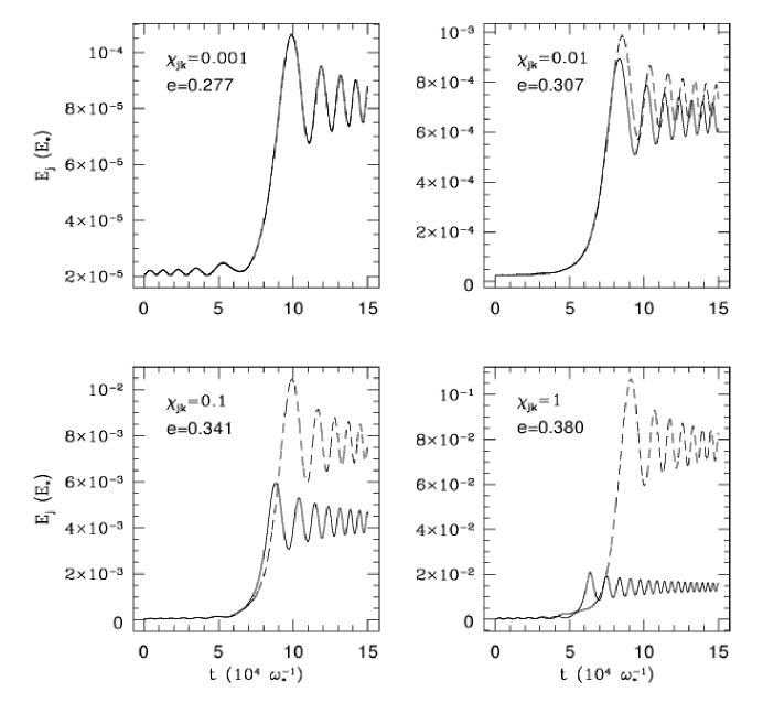
Figure 2: The energy in the $\ell=m=2$ f-mode on a $0.6$ $M_{\odot}$ white dwarf is shown for a passage through the $k=15$ resonance with different values of the parameter $\chi_{jk}$ obtained by varying the eccentricity, and with $q=10,000$. In each plot, the dashed curve is the system without back reaction, and the solid curve is the system with back reaction. The curves have been smoothed to remove high-frequency components.

The delineation of the back reaction and no back reaction regimes in the eccentricity-harmonic plane obtained with the above criterion for a quadrupolar f-mode on a $0.6$ $M_{\odot}$ white dwarf and various companion masses is shown in Figure 3. It is seen that the region of parameter space where back reaction may be neglected, according to the $\chi_{jk}$ criterion, grows with the companion mass. There is, however, a reason to think that back reaction might actually play an important role in some regions of the parameter space where the $\chi_{jk}$ criterion indicates otherwise.

Consider the following thought experiment. Imagine that we are approaching a resonance with an initial phase that would lead to a net negative energy transfer in the no back reaction approximation. As we start removing energy from the mode and depositing it into the orbit, the orbital frequency will necessarily decrease (i.e. the semi-major axis will increase) and the system will get pushed off resonance. It will then have another chance to approach the same resonance. Then, if the phase is such that energy is transferred to the mode, then the system will once again get pushed off resonance, but this time in the opposite direction (since the orbital frequency will increase). Gravitational radiation will then evolve the system away from this resonance and towards the next one. This scenario hints at the possibility that back reaction may force the resonant energy transfer to be always positive. However, this is not necessarily the case. For instance, we have assumed that there is sufficient initial energy in the mode to be able to change the orbital frequency significantly. Also, we have neglected the fact that gravitational radiation will be removing energy from the orbit as we are transferring energy to the orbit from the mode. If the rate of dissipation by gravitational radiation is high enough, then back reaction may not matter. The system will evolve through resonance regardless, on a time-scale determined by the rate of dissipation. Hence, we can still get a net negative energy transfer to the mode.

In summary, back reaction may be important in determining both the magnitude and the direction of resonant energy transfer. The $\chi_{jk}$ criterion provides, in some sense, only a measure of the correction to the magnitude. In the regime where $\chi_{jk}\gtrsim 1$, the implication is unambiguous: back reaction will be essential in determining the energy transfer. However, when $\chi_{jk}<1$, things are somewhat uncertain for reasons stated above. A solution of the problem including back reaction is required to determine conclusively whether back reaction is important in that regime.

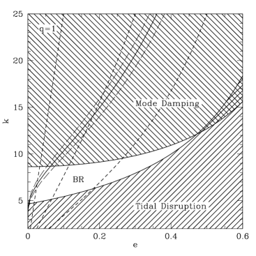
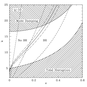
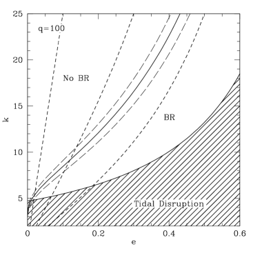
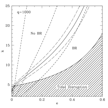
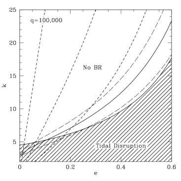
Figure 3: The regions in eccentricity-harmonic space where back reaction is and is not important (labelled as “BR” and “No BR”, respectively) are delineated according to the $\chi_{jk}$ criterion for a $\ell=m=2$ f-mode of a $0.6$ $M_{\odot}$ white dwarf, and various mass ratios. In each plot, the solid curve traces out the contour $\chi_{jk}=1$, and the long dashed lines to its left and right trace $\chi_{jk}=0.1$ and $\chi_{jk}=10$, respectively. The short dashed lines trace three gravitational radiation inspiral trajectories through the plane. For reference, the tidal limit and the region where mode damping via gravitational radiation during inspiral is important are also shown. Note that, for the mode damping curves, the full, eccentricity-dependent inspiral times have been used, rather than the circular orbit times.

5.2 Long term evolution

In §4, we calculated the energy transfer for an individual resonance in the absence of back reaction. In general, as the binary shrinks under gravitational radiation, the system will pass through a sequence of resonances for each mode. However, this is only a possibility for an eccentric orbit because, as demonstrated previously, only the fundamental resonance exists for a circular orbit. We note that, in the no back reaction approximation, the energy transfer at a resonance can be negative as well as positive, depending on the relative phase of the mode and the driver, and the initial amplitude. Also, there will be negligible average energy transfer between resonances, as long as we are well outside the tidal limit. If we assume (as seems reasonable) that the system has no long term phase memory, then the relative phasing at each resonance will be essentially random, with a uniform distribution. It then follows that, on average, the mode will tend to gain energy over time, and that the average total energy transfer after a sequence of resonances will be simply the sum of the individual average energy transfers given by (35).

Let $\varepsilon_{k}$ denote the average energy transfer given by (35) for a particular mode at the $k$-th resonance, and let $E_{k}$ be the energy (in units of $E_{*}$) in the mode before the $k$-th resonance. It then follows from (9) and our assumptions of random phases and negligible energy transfer between resonances that, for a sequence of resonances in the no back reaction approximation, the evolution of the mode energy will be given by the discrete random walk (with a drift)

$$E_{k-1}=E_{k}+\varepsilon_{k}\left(1+2\sqrt{\frac{E_{k}}{\varepsilon_{k}}}C_{k}\right)\ ,$$ (40)

where $C_{k}$ is a random variable drawn from the distribution

$$p(x)=\frac{1}{\pi\sqrt{1-x^{2}}}\ ,\quad x\in[-1,1]\ .$$

For a derivation of elementary statistical properties of this random walk, see Appendix D.

Figure 4 shows the results from calculations of passage through a sequence of resonances performed using the above random walk model for several sets of initial conditions. We have chosen to plot the mode amplitude

$$B_{j}\equiv\frac{1}{R_{\ast}}\sqrt{\frac{2E_{j}}{M_{j}\omega_{j}^{2}}}\ ,$$ (41)

rather than the energy, because we want to draw attention to the fact that, for moderate initial eccentricities, the amplitude of a $\ell=m=2$ f-mode can be driven to values in the range $\sim$0.1–1. (An amplitude of unity for a $\ell=m=2$ mode corresponds to a maximum physical displacement of the stellar surface of about 55% relative to the unperturbed radius.) We therefore expect that the linear normal mode analysis might not be valid in those cases, and that non-linear effects may in fact determine the actual outcome.

Figure 4: The amplitude of a $\ell=m=2$ f-mode of a $0.6$ $M_{\odot}$ white dwarf during passage through a sequence of resonances in the no back reaction approximation is shown for several sets of initial conditions. All of these lie in regions of the eccentricity-harmonic plane where back reaction is not important according to the $\chi_{jk}$ criterion. The calculations were done using our semi-analytical formalism. In each case, the solid line shows a particular realization of the random walk given by (40), and the dashed line follows the ensemble average. The random walks were terminated when $\chi_{jk}\sim 0.01$. Note that the scales on the axes are different for each plot.

It should be noted that, even if back reaction plays a role in determining the direction of energy transfer, our result that non-linear amplitudes for a $\ell=m=2$ f-mode can be attained by passage through a sequence of resonances is unlikely to be affected. This is due to the fact that the result depends chiefly upon the allowed magnitude of energy transfer, and as we restricted our calculations to the regime where $\chi_{jk}\ll 1$, back reaction is not expected to change things.

6 Conclusions

In this paper, we have discussed a specific dynamical problem: what is the energy transfer to the normal modes of a white dwarf due to tidal resonances in a compact object binary inspiralling under gravitational radiation? For simplicity, we have considered only non-rotating, completely degenerate stellar models. We have provided a semi-analytical answer for the case when the perturbation of the orbit by the modes may be neglected (the no back reaction approximation). It has been shown that, ignoring back reaction, and assuming that the relative phase of the mode and the orbit is randomised between successive resonances, the energy in a mode executes a discrete random walk, with a drift, during passage through a sequence of resonances. In addition, we have found that the amplitude of a $\ell=m=2$ f-mode can be driven into the non-linear regime as a result of passage through such a sequence. We have also demonstrated that back reaction can modulate the amount of energy transferred significantly, depending upon the parameters of the system. Our attempt to delineate the regime in parameter space where the no back reaction approximation is valid has had mixed success: we can predict when back reaction will be definitely important, but a clear delineation of the regime where it will be unimportant has not been found. Despite this ambiguity, our result that non-linear amplitudes can be attained for a $\ell=m=2$ f-mode is expected to be robust. A treatment of the problem including back reaction will be the subject of a future publication.

Appendix A Details of Calculation for Forced Harmonic Oscillator

From (5) and (8), it follows that

$$\begin{split}\zeta_{1}=\frac{F_{R}}{2}e^{i\omega_{0}\tau}\int_{\tau_{0}}^{\tau}&d\tau^{\prime}\,\bigg{\{}\exp\left[i\left(\phi_{R}+\alpha\frac{\omega_{0}^{2}\tau^{\prime 2}}{2}\right)\right]\\ &+\exp\left[-i\left(\phi_{R}+2\omega_{0}\tau^{\prime}+\alpha\frac{\omega_{0}^{2}\tau^{\prime 2}}{2}\right)\right]\bigg{\}}\ .\end{split}$$

Completing the square in the argument of the second exponential, we get

$$\begin{split}\zeta_{1}=\frac{F_{R}}{2}e^{i\omega_{0}\tau}\Bigg{\{}&I_{1}(\tau)\exp\left(i\phi_{R}\right)\\ &+I_{2}(\tau)\exp\left[-i\left(\phi_{R}-\frac{2}{\alpha}\right)\right]\Bigg{\}}\ ,\end{split}$$

where

$$I_{1}(\tau) \equiv\int_{\tau_{0}}^{\tau}d\tau^{\prime}\,\exp\left(\frac{i}{2}\alpha\omega_{0}^{2}\tau^{\prime 2}\right)\ ,$$

$$I_{2}(\tau) \equiv\int_{\tau_{0}}^{\tau}d\tau^{\prime}\,\exp\left[-\frac{i}{2}\left(\sqrt{\alpha}\omega_{0}\tau^{\prime}+\frac{2}{\sqrt{\alpha}}\right)^{2}\right]\ .$$

Making the change of variables

$$u(\tau^{\prime}) \equiv\sqrt{\frac{\alpha}{\pi}}\omega_{0}\tau^{\prime}\ ,$$

$$v(\tau^{\prime}) \equiv\sqrt{\frac{\alpha}{\pi}}\omega_{0}\tau^{\prime}+\frac{2}{\sqrt{\pi\alpha}}\ ,$$

we have

$$I_{1} =\frac{1}{\omega_{0}}\sqrt{\frac{\pi}{\alpha}}\int_{u_{0}}^{u_{\tau}}du\,\exp\left(\frac{i\pi u^{2}}{2}\right)\ ,$$

$$I_{2} =\frac{1}{\omega_{0}}\sqrt{\frac{\pi}{\alpha}}\int_{v_{0}}^{v_{\tau}}dv\,\exp\left(-\frac{i\pi v^{2}}{2}\right)\ ,$$

where $u_{0}=u(\tau_{0})$, $u_{\tau}=u(\tau)$, et cetera. Evaluating the integrals gives

$$I_{1} =\frac{1}{\omega_{0}}\sqrt{\frac{\pi}{\alpha}}\Big{\{}C(u_{\tau})-C(u_{0})+i\left[S(u_{\tau})-S(u_{0})\right]\Big{\}}\ ,$$

$$I_{2} =\frac{1}{\omega_{0}}\sqrt{\frac{\pi}{\alpha}}\Big{\{}C(v_{\tau})-C(v_{0})-i\left[S(v_{\tau})-S(v_{0})\right]\Big{\}}\ ,$$

where the Fresnel integrals are defined by

$$C(z) \equiv\int_{0}^{z}dt\,\cos\left(\frac{\pi t^{2}}{2}\right)\ ,$$

$$S(z) \equiv\int_{0}^{z}dt\,\sin\left(\frac{\pi t^{2}}{2}\right)\ .$$

Note that

$$\lim_{z\rightarrow\pm\infty}C(z)=\lim_{z\rightarrow\pm\infty}S(z)=\pm\frac{1}{2}$$

(see, for example, Abramowitz & Stegun, 1972). Let us now consider the energy after long times. If we start out from zero frequency, then $\omega_{0}\tau_{0}=-\alpha$, and

$$u_{0} =-\frac{1}{\sqrt{\pi\alpha}}\ll-1\ , v_{0} =\frac{1}{\sqrt{\pi\alpha}}\gg 1\ .$$

The $I_{2}$ integral will not contribute significantly since its upper and lower limits are effectively the same. For $I_{1}$, we find

$$I_{1}=\frac{1}{\omega_{0}}\sqrt{\frac{\pi}{\alpha}}\left(1+i\right)=\frac{1}{\omega_{0}}\sqrt{\frac{2\pi}{\alpha}}e^{i\pi/4}\ .$$

Hence, after some algebra,

$$\Delta E\equiv E-E_{0}=\frac{\pi F_{R}^{2}}{4\alpha\omega_{0}^{2}}\left(1+2\sqrt{\frac{E_{0}}{\pi F_{R}^{2}/4\alpha\omega_{0}^{2}}}\cos\psi\right)\ ,$$

where $E_{0}=\left|\zeta_{0}\right|^{2}/2$ and $\psi$ is an initial phase.

Appendix B Hansen Coefficients

The Hansen coefficients $X_{k}^{p,m}$ for the two-body problem are defined by

$$\left(\frac{R}{a}\right)^{p}\exp(imv)=\sum_{k=-\infty}^{\infty}X_{k}^{p,m}(e)\exp(ikl)\ ,$$

where $R$ is the orbital separation, $a$ is the semi-major axis, $v$ is the true anomaly, $e$ is the orbital eccentricity, and $l$ is the mean anomaly. The Hansen coefficients are real functions of the eccentricity, and it can be shown that, to lowest order in eccentricity,

$$X_{k}^{p,m}(e)\propto e^{\left|k-m\right|}$$

(Murray & Dermott, 1999, and references therein). The coefficients can be calculated to any desired order in eccentricity as a series in terms of Newcomb operators:

$$X_{k}^{p,m}(e)=e^{\left|k-m\right|}\sum_{\nu=0}^{\infty}X^{p,m}_{\nu+\lambda,\nu+\zeta}e^{2\nu}\ ,$$

where $\lambda=\max(0,k-m)$, $\zeta=\max(0,m-k)$, and the Newcomb operators $X^{a,b}_{c,d}$ are defined via recursion relations (see Murray & Dermott, 1999). Alternatively, for quantitative work, the Hansen coefficients can be evaluated for a given eccentricity by calculating the integral

$$X_{k}^{p,m}(e)=\frac{1}{2\pi}\int_{0}^{2\pi}dl\,\left(\frac{R}{a}\right)^{p}\cos(mv-kl)$$

numerically.

Appendix C Damping of Quadrupolar Modes Under Gravitational Radiation

The average power radiated in gravitational waves due to a time-dependent mass quadrupole moment is given, in the weak-field limit of general relativity, by

$$\frac{dE_{\rm GW}}{dt}=\frac{G}{45c^{5}}\langle\dddot{Q}_{ij}\dddot{Q}_{ij}\rangle$$

(Misner et al., 1973), where $Q_{ij}$ is the mass quadrupole moment as defined conventionally in classical physics:

$$Q_{ij}=\int d^{3}x\,\left(3x_{i}x_{j}-r^{2}\delta_{ij}\right)\rho(\mathbf{x},t)\ .$$

It can be shown that the power radiated by a quadrupolar mode is independent of $m$ (this is a consequence of the Wigner-Eckart theorem). Hence, we can restrict ourselves to the $m=0$ case for simplicity. It then follows that $Q_{11}=Q_{22}=-Q_{33}/2$, and that the off-diagonal terms vanish. Therefore, noting that the time dependence is sinusoidal, we have

$$\frac{dE^{\rm GW}_{j}}{dt}=-\frac{G}{60c^{5}}\omega_{j}^{6}\dddot{Q}_{33}^{2}\ ,$$ (42)

where $Q_{33}$ should now be understood to mean the time-independent amplitude of the mass quadrupole moment. Writing the mass density as

$$\rho(\mathbf{x})=\rho_{0}(r)+B_{j}\delta\rho_{j}(r)Y_{20}(\mathbf{\hat{r}})\ ,$$

where $B_{j}$ is the amplitude of the mode and $\delta\rho_{j}$ is the normalised density perturbation associated with the mode, we find

$$Q_{33}=4\sqrt{\frac{\pi}{5}}B_{j}\int_{0}^{R_{\ast}}dr\,r^{4}\delta\rho(r)\ .$$

The above integral can be simplified by using the linearised Poisson equation, integrating by parts twice, and using the surface boundary condition $\eta_{4}=-(\ell+1)\eta_{3}$. The result is

$$Q_{33}=\sqrt{\frac{5}{\pi}}M_{\ast}R_{\ast}^{2}\eta_{3j}(R_{\ast})B_{j}\ .$$

Substituting the above expression into (42), we get

$$\frac{dE^{\rm GW}_{j}}{dt}=-\frac{GM_{\ast}^{2}R_{\ast}^{4}}{12\pi c^{5}}\eta_{3j}^{2}(R_{\ast})\omega_{j}^{6}B_{j}^{2}\ .$$

Finally, noting that the total energy for an isolated mode is given by

$$E_{j}=\frac{1}{2}M_{j}R_{\ast}^{2}\omega_{j}^{2}B_{j}^{2}\ ,$$

we arrive at the $e$-folding time for the mode energy under damping by gravitational radiation:

$$T_{j}=\frac{6\pi}{\omega_{\ast}}\beta_{\ast}^{-5}\eta_{3j}^{-2}(R_{\ast})\left(\frac{M_{j}}{M_{\ast}}\right)\sigma_{j}^{-4}\ .$$

Appendix D Statistical Properties of Resonant Energy Transfer in the No Back Reaction Approximation

In this appendix, we derive some statistical properties of the random walk given by (40), which we rewrite as

$$E_{k-1}=E_{k}+\varepsilon_{k}+Z_{k}\ ,$$ (43)

where

$$Z_{k}\equiv 2\sqrt{\varepsilon_{k}E_{k}}C_{k}\ .$$

Recall that $\varepsilon_{k}$ is known in advance, and that $C_{k}$ is a random variable drawn from the distribution

$$p(x)=\frac{1}{\pi\sqrt{1-x^{2}}}\ ,\quad x\in[-1,1]\ .$$

Note that

$$\langle C_{k}\rangle=0\ ,\quad\langle C_{k}^{2}\rangle=\frac{1}{2}\ .$$

Since $E_{k}$ will only depend upon $C_{\alpha}$, for $\alpha>k$, $Z_{k}$ is linear in $C_{k}$. As all the $C_{k}$ are independent random variables (by assumption), it follows that

$$\langle Z_{k}\rangle=0\ ,\quad\langle Z_{k}^{2}\rangle=2\varepsilon_{k}\langle E_{k}\rangle\ .$$ (44)

Given an initial mode energy $E_{k}$ before the $k$-th resonance, we wish to determine the average mode energy $\langle E_{k-p}\rangle$, and its variance $\sigma_{p}^{2}$, after passage through $p$ resonances. From (43), we have

$$E_{k-p}=E_{k}+\sum_{\alpha=k-p+1}^{k}\varepsilon_{\alpha}+\Delta_{p}\ ,$$ (45)

where we have defined

$$\Delta_{p}\equiv\sum_{\alpha=k-p+1}^{k}Z_{\alpha}\ .$$

Using (44), it follows immediately that

$$\langle E_{k-p}\rangle=E_{k}+\sum_{\beta=k-p+1}^{k}\varepsilon_{\beta}\ .$$ (46)

Note that, since $\varepsilon_{\beta}>0$, $\langle E_{k-p}\rangle$ increases monotonically as we pass through a sequence of resonances. Hence, we say that the random walk (43) has a drift. To calculate the variance, we need to find $\langle E_{k-p}^{2}\rangle$. Writing

$$\begin{split}E_{k-p}^{2}=\left(E_{k}+\sum_{\alpha=k-p+1}^{k}\varepsilon_{\alpha}\right)^{2}+\Delta_{p}^{2}+O(\Delta_{p})\ ,\end{split}$$

we see that

$$\langle E_{k-p}^{2}\rangle=\langle E_{k-p}\rangle^{2}+\langle\Delta_{p}^{2}\rangle\ ,$$ (47)

as all the terms linear in $\Delta_{p}$ will vanish when averaged. To calculate $\langle\Delta_{p}^{2}\rangle$, we write

$$\Delta_{p}^{2}=\sum_{\alpha=k-p+1}^{k}Z_{\alpha}^{2}+2\sum_{\alpha=k-p+1}^{k-1}\sum_{\beta=\alpha+1}^{k}Z_{\alpha}Z_{\beta}\ ,$$

and note that, since $\beta>\alpha$ in the above double sum, each term of the double sum will be linear in $C_{\alpha}$, and will, hence, vanish upon averaging. Therefore, we have

$$\langle\Delta_{p}^{2}\rangle=2\sum_{\alpha=k-p+1}^{k}\varepsilon_{\alpha}\langle E_{\alpha}\rangle\ .$$

Substituting into (47), and then using (46), we find

$$\sigma_{p}^{2}=2\sum_{\alpha=k-p+1}^{k}\varepsilon_{\alpha}\left(E_{k}+\sum_{\beta=\alpha+1}^{k}\varepsilon_{\beta}\right)\ .$$ (48)

It should be noted that (43) is not Gaussian, nor will it become Gaussian after many resonances. That the process is not Gaussian is clear from the fact that the random walk is bounded from below. Furthermore, the central limit theorem is not applicable because, typically, the probability distribution of $\Delta_{p}$ is dominated by the most recent few harmonics, and hence the effective number of variables never becomes large.

References

- Abramowitz & Stegun (1972) Abramowitz M., Stegun I. A., eds, 1972, Handbook of Mathematical Functions. Dover, New York
- Arfken & Weber (1995) Arfken G. B., Weber H. J., 1995, Mathematical Methods for Physicists. Academic Press, San Diego
- Bildsten & Cutler (1992) Bildsten L., Cutler C., 1992, ApJ, 400, 175
- Bromm et al. (1999) Bromm V., Coppi P. S., Larson R. B., 1999, ApJ, 527, L5
- Colbert & Mushotzky (1999) Colbert E. J. M., Mushotzky R. F., 1999, ApJ, 519, 89
- Colbert & Ptak (2002) Colbert E. J. M., Ptak A. F., 2002, ApJS, 143, 25
- Dziembowski (1982) Dziembowski W., 1982, Acta Astronomica, 32, 147
- Edwards & Bailes (2000) Edwards R., Bailes M., 2000, ApJ, 547, L37
- Eggleton (1983) Eggleton P. P., 1983, ApJ, 268, 368
- Fabian et al. (1975) Fabian A. C., Pringle J. E., Rees M. J., 1975, MNRAS, 172, 15P
- Finn & Thorne (2000) Finn L. S., Thorne K. S., 2000, Phys. Rev. D, 62, 124021
- Gingold & Monaghan (1980) Gingold R. A., Monaghan J. J., 1980, MNRAS, 191, 897
- Hills (1977) Hills J. G., 1977, AJ, 82, 626
- Iyer & Will (1995) Iyer B. R., Will C. M., 1995, Phys. Rev. D, 52, 6882