A STUDY OF PROMPT EMISSION MECHANISMS IN GAMMA-RAY BURSTS
Abstract
The principal paradigm for the generation of the non-thermal particles that are responsible for the prompt emission of gamma-ray bursts invokes diffusive shock acceleration at shocks internal to the dynamic ultrarelativistic outflow. This paper explores expectations for burst emission spectra arising from shock acceleration theory in the limit of particles cooling much slower than their acceleration. Parametric fits to burst spectra obtained by the Compton Gamma-Ray Observatory (CGRO) are explored for the cases of the synchrotron, inverse Compton and synchrotron self-Compton radiation mechanisms, using a linear combination of thermal and non-thermal electron populations. These fits demand that the preponderance of electrons that are responsible for the prompt emission reside in an intrinsically non-thermal population, strongly contrasting particle distributions obtained from acceleration simulations. This implies a potential conflict for acceleration scenarios where the non-thermal electrons are drawn directly from a thermal gas, unless radiative efficiencies only become significant at highly superthermal energies. It is also found that the CGRO data preclude effective spectroscopic discrimination between the synchrotron and inverse Compton mechanisms. This situation may be resolved with future missions probing gamma-ray bursts, namely Swift and GLAST. However, the synchrotron self-Compton (SSC) spectrum is characteristically too broad near the peak to viably account for bursts such as GRB 910601, GRB 910814 and GRB 990123. It is concluded that the SSC mechanism may be generally incompatible with differential burst spectra steeper than around above the peak, unless the synchrotron component is strongly self-absorbed.
Department of Physics and Astronomy MS-108,
Rice University, P.O. Box 1892, Houston, TX 77251, U.S.A.
baring@rice.edu
and
Department of Physics, Washington University
One Brookings Drive, St. Louis, MO 63130, U.S.A.
mbraby@hbar.wustl.edu
To appear in The Astrophysical Journal, Vol 613, September 20, 2004 issue.
Subject headings: gamma-rays: bursts — radiation mechanisms: non-thermal — gamma rays: theory — relativity
1 INTRODUCTION
Cosmological gamma-ray bursts are one of the most interesting and exotic phenomena in astrophysics. In standard burst models (e.g. see Piran 1999; Mészáros 2001 for reviews), the rapidly expanding fireball decelerates, converting the internal energy of the hot plasma into kinetic energy of the beamed, relativistically moving ejecta and electron-positron pairs. At the point where the fireball becomes optically thin and the gamma-ray burst (GRB) we see is emitted, the matter will not emit non-thermal gamma-rays unless some mechanism can efficiently re-convert the kinetic energy back into internal energy, i.e., unless some particle acceleration process takes place. Diffusive shock acceleration is widely believed to be this mechanism (e.g., Rees & Mészáros 1992; Piran 1999) for the prompt emission; it is also likely to be a key element for the underlying physics of X-ray and optical flashes and burst afterglows.
An important question concerning burst models is whether or not their prompt emission can be accurately described by a detailed shock acceleration analysis, and if so, how is the pertinent parameter space of models limited by the observations? Tavani (1996a,b) proposed a synchrotron shock emission model that invoked such diffusive acceleration as the means for generating non-thermal distributions. This work has been an interpretative driver in the field, due in part to the impressive model fits of data he obtained. Yet, Tavani’s model and many subsequent works do not treat the critical involvement the acceleration process has on shaping the relationship between the thermal and non-thermal portions of the electron distribution. The normal approach is to simplify the distribution to a truncated or broken power-law, occasionally with an additional thermal component. The viability of the synchrotron model, or emission scenarios that invoke any other radiation mechanism, hinges on such subtleties of the particle distribution, which are inextricably linked to the nature of shock acceleration, diffusive or coherent. In addition, they must provide compatibility with the hard X-ray spectral index, an issue raised by Preece et al. (1998; 2000), who observed that around 1/3 of all BATSE bursts exhibited spectra that were too flat below the peak to accommodate a synchrotron interpretation.
This paper explores the general expectations for burst emission spectra from shock acceleration theory. Parametric descriptions for a linear combination of thermal and non-thermal distributions are used to obtain fits to burst spectra for the cases of the synchrotron, inverse Compton and synchrotron self-Compton (SSC) mechanisms, and these distributions are interpreted in the context of known results from acceleration simulations. Cases of particles cooling much slower than their acceleration are treated in this exposition; justification for these are discussed in Section 2.6. The focus is on GRBs observed by the Compton Gamma-Ray Observatory, specifically those with EGRET detections that provide broad spectral coverage and therefore more constrained fits around the spectral peak. It is found that acceptable fits are only possible with a marked dominance of non-thermal electrons, contrasting the particle distributions obtained in acceleration simulations. This poses a general problem for any burst acceleration paradigm where the non-thermal population is drawn probabilistically from a thermal gas.
In addition, fits are found to be more or less equally acceptable for the synchrotron and inverse Compton processes; it is anticipated that Swift will provide a number of bright bursts where spectral fitting down into the X-ray band might enable discrimination between such emission mechanisms. However, at this juncture, spectroscopic discrimination against unabsorbed synchrotron self-Compton scenarios seems probable, given that the characteristically broad SSC spectra in space are difficult to reconcile with CGRO data. In service of this analysis, a compact formalism for SSC emissivities from thermal and truncated power-law electron distributions is present in the Appendix. It is anticipated that GLAST’s broad spectral coverage from keV to GeV, supplied by the Gamma-Ray Burst Monitor in the BATSE band and the Large Area Telescope in and above the EGRET band, will render GLAST a powerful tool in constraining and interpreting burst spectral properties in the future.
2 SYNCHROTRON EMISSION AND ITS INTERPRETATION
This section explores the relationship of synchrotron spectra to the electron energy and angular distributions, inferring Lorentz factor distributions using data from the bright burst GRB 910503 as a representative case study.
2.1 Synchrotron Formalism and Electron Distributions
The formalism for synchrotron radiation in optically thin environs is standard and readily available in many textbooks, including the treatments of Bekefi (1966), Jackson (1975) and Rybicki & Lightman (1979). Throughout this paper, the standard convention for the labelling of the photon polarizations will be adopted, namely that refers to the state with the photon’s electric field vector parallel to the plane containing the magnetic field and the photon’s momentum vector, while denotes the photon’s electric field vector being normal to this plane.
The classical (photon) angle-integrated emissivities for the and polarization for monoenergetic electrons of Lorentz factor moving at angle to the field are (e.g. Westfold 1959; Jackson 1975; Rybicki and Lightman 1979)
in units of , where the are modified Bessel functions of the second kind. The generally higher probability of emitting photons than ones reflects the intrinsic dipolar radiative nature of accelerating/oscillating charges; the polarization is elliptical for photon propagation along the field. The characteristic synchrotron rate factor that scales these emissivities is
| (2) |
Here, is the fine structure constant. The photon energies that appear in these functions that form the scaling for the energies of emission are [with the electron Compton wavelength over being ]:
| (3) |
where is the particle’s Larmor radius, and Gauss is the quantum critical field. Note that since , the photon angles to the field form a narrow distribution about . Furthermore, the expressions in Eq. (2.1) are appropriate for cases where the particle momenta are not closely aligned with the magnetic field; situations of such near alignment are discussed in Section 2.5 below.
The total synchrotron emissivity is obtained by integrating over the energy and angular distribution of the particles. For electron distributions in units of , summing over polarizations forms the expression for the emissivity that will be used mostly throughout this paper (in units of ):
| (4) |
This is the differential photon spectrum; frequently in this work, reference will be made to the so-called spectrum, a spectral energy distribution that is proportional to .
Physical diagnostics on the GRB environment are obtained by comparing the emission spectrum in Eq. (4) with observations. The obvious database of choice comprises BATSE observations from the Compton Gamma-Ray Observatory (CGRO), specifically the BATSE spectroscopy catalog of Preece et al. (2000) with its pubicly-accessible electronic compilation. Yet this data possesses a principal limitation, namely that imposed by the restricted energy band of BATSE. Inferences of particle distributions are generally on a more secure footing when using broader burst spectra, particularly in domains of significant spectra structure, which is the intrinsic nature of the BATSE pool. Thus, the two decades of energy afforded by BATSE often are insufficient to describe the nature of the non-thermal particle distribution invoked in models. Data from the EGRET experiment on CGRO suitably augment this situation and extend the dynamic range by 2–4 orders of magnitude in energy. Accordingly, a focus on EGRET bursts is insightful and offers more secure determinations of particle distributions. Use is therefore made of spectral compilations of BATSE, COMPTEL and EGRET data that are offered in Schaefer et al. (1998). Specifically, a case study is made here of GRB 910503, observing that the inferences to be made generally extend to the handful of other EGRET bursts, and also to a large number of bright BATSE bursts that possess no confirmed EGRET detections.
Note that the focus here is primarily on time-integrated spectra. Given the complexity and diversity of burst time profiles, and associated variations in spectral shape and the well-known hard-to-soft evolution, detailed spectral fits will depend on the time window chosen. A classic example for this is provided by the gradual emergence of a hard gamma-ray component in the spectrum of GRB 941017 (Gonzalez, et al. 2003). The main conclusions of this paper apply to the mean properties of the emitting particle distributions, and are striking enough to indicate their applicability for most or nearly all of the duration of the bursts studied herein.
A variety of particle distributions are possible in modeling burst spectra. Clearly, all should contain a non-thermal component, since the data are clearly non-thermal: purely isothermal models do not work (Pacynski 1986; Goodman 1986), though constructed convolutions of thermal spectra of different temperatures are possible. The emphasis here is motivated by physical interpretation, and the leading contender for non-thermal particle energization in bursts is diffusive acceleration at relativistic shocks in the burst outflow. Such acceleration is well studied in non-relativistic flows, and is widely believed to originate with thermal particles that are diffusively transported when interacting with field turbulence in the shock environs. Such transport effects many crossings of the shock layer (e.g. see Drury 1983; Blandford & Eichler 1987; Jones & Ellison 1991 for reviews), that lead to a friction term in the momentum evolution, i.e. acceleration. While other acceleration models such as reconnection and coherent electrodynamic energization exist and are appropriate in a variety of astrophysical environments (e.g. the solar corona, pulsar magnetospheres), diffusive shock acceleration is the most widely invoked in astrophysical models; it forms the centerpiece of discussion here as well as for many investigations of bursts.
Tavani (1996a,b) proposed a shock emission model that invoked such diffusive acceleration as the means for generating non-thermal distributions. This work has been an interpretative driver in the field, in no small part due to the impressive model fits of data obtained. The principal purpose of this Section is to delve deeper into the physical implications of such data fitting. Accordingly, it is appropriate to use an electron distribution similar to Tavani’s (1996a,b) to add insight to the discussion. Here, the quasi-isotropic electron distribution
| (5) |
is adopted, where is a step function with for and zero otherwise, and is the system or post-shock temperature. The factor directly relates to the efficiency of acceleration, and is a parameter in the fitting protocol, as are (assumed much greater then unity), the dimensionless , the non-thermal index , and the normalization factor . The ensuing discussion will provide physical grounds justifying this choice of distribution in shocked environs; other possibilities with different mandates include the broken power-law adopted by Lloyd & Petrosian (2000). Note that is independent of for true isotropy. In many cases in this paper, will be chosen for simplicity, since this corresponds to the dominant radiative contribution from the synchrotron mechanism.
The parameter is introduced to generalize from Tavani’s (1996a,b) fits, permitting the non-thermal distribution to emerge perhaps at truly super-thermal energies, rather than exactly in the thermal peak (Tavani’s restricted case). Typical acceleration spectra in non-relativistic shocks assume forms similar in general appearance to Eq. (5). Specifically, they correspond to the portion of parameter space (at least for ions), so that dissipation in the shock layer leads to a heating plus non-thermal acceleration that ensues only at super-thermal energies in the Maxwell-Boltzmann tail. Evidence for such a structured distribution can be found both in heliospheric measurements of accelerated ions near shocks (e.g. Earth’s Bow Shock: see Ellison, Möbius & Paschmann 1990; interplanetary shocks: see Baring et al. 1997), and also a variety of acceleration simulations and theoretical analyses (e.g. see Scholer, Trattner & Kucharek 1992; Giacalone et al. 1993, Baring, Ellison & Jones 1993; Ellison, Baring & Jones 1996; Kang & Jones 1997). The situation for relativistic shocks is less certain, due in no small part to the absence of in situ spacecraft determinations of particle spectra; simulation expectations for such environments are discussed below. In this paper, values of appear, being in general only weakly constrained by the fits and largely motivated by the above physical and theoretical considerations.
While numerical evaluations of Eq. (4) given the electron distribution in Eq. (5) were performed to obtain approximations to burst spectra, standard asymptotic limits are readily attainable in analytic form. The non-thermal contribution to the synchrotron spectrum (from the truncated power-law), dominant whenever , assumes the following power-law forms (derived, for example, from Eq. [11]):
| (6) |
Here, is the component of the field perpendicular to the instantaneous electron motion. The thermal component, sampled when , necessarily declines exponentially at photon energies well above the thermal peak, but possesses the same power-law dependence as in the non-thermal case for low photon energies:
| (7) |
This spectral similarity at low energies follows from the narrow nature of the distributions being convolved with the synchrotron emissivity functions in Eq. (2.1). Accordingly, it is not possible to distinguish between emission from thermal or power-law distributions if spectrum measurements exist only at energies below the peak; some other diagnostic is required. The exponential decline above the thermal peak possesses a somewhat complex two-domain structure; the reader is referred to Pavlov & Golenetskii (1986), Brainerd & Petrosian (1987) and Baring (1988a) for the presentation of appropriate asymptotic forms in cases .


It must be noted that throughout this paper, photon spectra are generated in the shock rest frame (SRF) and then boosted in energy to the observer’s frame (OF) by a fixed Doppler factor, independent of photon angle in the SRF. This approximation, essentially adopted in many models of GRB spectra, is expedient but does not accommodate the fact that photon distributions in the SRF are inherently anisotropic due both to the instrinsic nature of the synchrotron and inverse Compton processes, and also to the fact that relativistic shocks naturally generate anisotropic ions and electrons. Notwithstanding, this boost approximation does not dramatically distort the angle-integrated OF spectral shape for typical SRF angular distributions and suffices to describe the continuum for the purposes of the discussions here.
2.2 Inferred Electron Distributions
Before presentation of results, it is appropriate to address the modeling procedure used in this paper. Approximate spectra, as opposed to data fits, were derived visually using both log-log and semi-log representations of spectra to increase confidence in the results. Least squares trials were performed in some cases, but with no addition of insight or perceived accuracy. This choice of a visual approach was one of expediency, and did not compromise the scientific conclusions presented here; the essential points are unambiguously made without the need of statistical analysis. This latitude is afforded by the limited energy range of the data in the BATSE catalog: slight adjustments in parameters used to fit the extant data for a given burst would almost certainly have been dominated by those needed to accommodate a broader spectral range. For the specific cases of GRB 910503 and GRB 910601, where EGRET data are incorporated in the study, the uncertainty in the MeV data points is a major contributor to the determination of model parameters. In bursts where no EGRET or COMPTEL data were used, the “fit” was actually to the Band (1993) model spectral fit presented in the Preece et al. (2000) spectroscopy catalog, not to the actual data. In such cases, the high energy Band model index was adopted, and other distribution parameters adjusted. In this sense, there was in implicit second order incorporation of the statistics embodied in the Band model fit. It must be emphasized that there is no uniquely preferred method for statistically fitting public data since it is already a convolution of model and instrumental response. The correct approach (as in Lloyd & Petrosian 2000) would be to fold spectral models here through the BATSE or EGRET detector response function, an enterprise that rapidly becomes more ambitious when different instrumental responses must be blended. Such complexity seems premature for the explorations of this paper, and is deferred until the more refined data of Swift and GLAST becomes available.
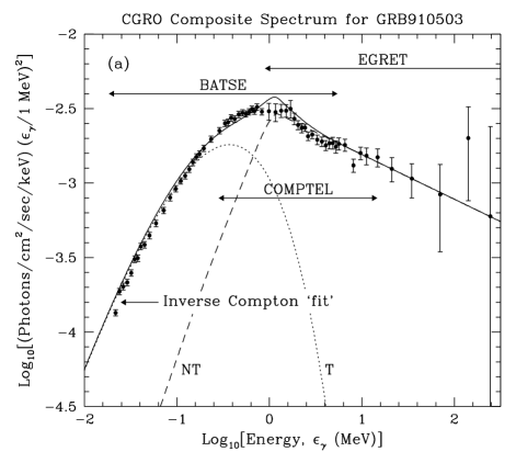
Results for the spectral approximation of the GRB 910503 data are presented in Figure 1, together with the multi-instrument, time-integrated CGRO data as provided by Schaefer (private communication) prior to the public release in Schaefer et al. (1998). We remark that the spectral deconvolutions published in Schaefer et al. (1998) were made independently for each data set from the different CGRO instruments, applying an artificial normalization to reconcile offsets in the different data amplitudes. Such a procedure is less accurate than a joint spectral deconvolution of the entire spectral data set (see for example the analysis of GRB 990123 data in Briggs et al. 1999). Notwithstanding, the major conclusions of this paper are robust and are not affected by such subtleties of data analysis.
Figure 1 displays both synchrotron emission spectra for the case of pitch angles (the so-called quasi-isotropic case), and the inferred electron distribution that generates the continuum. For the solid curve approximate case, the overall normalization is obviously a free parameter and was offset slightly from the data for visual clarity. The electron distributions were normalized to unit area in space. The solid curve depicts the case that would be required to explain the photon spectrum. The non-thermal particle distribution clearly dominates the thermal component in this “fit.” Its index differs from the value of 3.8 that Tavani (1996a) obtained in his analysis of this burst, a discrepancy that is actually insignificant given the error bars in the EGRET data. Adjustment of the parameter to improve the appearance of the model approximation around and above the spectral peak led to the assumed value of , accurate to around 15%. Notwithstanding, there appears to be some spectral structure around the peak that cannot be explained by the simple particle distribution in Eq. (5). The positioning of the peak in energy produced the fit value , where is the Lorentz factor associated with the bulk motion of the GRB expansion. Here, is interpreted as the magnetic field in the burst expansion frame, i.e., not in the ISM or shock rest frames.
The parameter describing the relative normalization of the non-thermal and thermal components was found to be (10%), a strikingly large value that is not addressed explicitly in detail by Tavani (1996a). A discussion of the implications of an inferred particle distribution with such a large follows just below. A similar property is obtained for synchrotron model fits for BATSE bursts GRB 940619 (trigger number 3035_6) and GRB 940817 (trigger number 3128_5) from the Preece et al. (2000) catalog, and also for GRB 910601 and GRB 910814 whose composite spectra are presented in Schaefer et al. (1998). The spectra for bursts GRB 930131 and GRB 940217 that possess EGRET detections also suggest a similar result, though the lack of a composite broad-band multi-instrument spectrum for each in the literature precluded a detailed analysis. The parameter regime of is expected to be pervasive for BATSE bursts, due to the smoothness of their circumpeak continua. For comparative purposes, another distribution and its resultant synchrotron is illustrated in Figure 1 as dashed curves. The distribution was deliberately chosen to possess a somewhat dominant thermal component, motivated by expectations from shock acceleration theory, and clearly yields a spectrum that grossly deviates from the observations both well above and well below the peak. While these deductions are obtained using a time-integrated spectrum, such a conclusion must apply either for most of the burst duration, or at sub-intervals when the burst was at its brightest.
For the synchrotron mechanism to be a viable explanation of GRB spectra, the underlying particle distribution must be physically realistic. Here, expectations of particle distributions from shock acceleration theory are the predominant focus, partly because this was the preferred acceleration mechanism in Tavani (1996a,b), and largely because this is the underlying energization assumed in most burst models. In a nutshell, both theory and observation pertaining to non-relativistic shocks strongly indicate and cases. Note that is essentially the parameter that demarcates the relative normalization of the non-thermal and thermal components in Equation (5).
Applications of shock acceleration in the heliosphere and at supernova remnant shells more or less mandate these parameter regimes, since the seed pool of particles that can be subjected to acceleration are thermal and moreover plentiful. In heliospheric environs, the source is the cold solar wind, and there is little evidence of significant pre-heating that is not connected to the shock system under study. The in situ spacecraft measurements exhibit strong heating at shocks and the generation of dominant thermal ions in the downstream regions, corresponding to cases. Data taken at the high sonic Mach number Earth’s bow shock (e.g. see Ellison, Möbius & Paschmann 1990; Scholer, Trattner & Kucharek 1992) and low sonic and Afvénic Mach number interplanetary shocks (e.g. see Gosling et al. 1981; Baring et al. 1997) clearly support this assertion. In supernova remnants, direct particle measurements are, or course, impossible, and inferences can only be made from radiative signatures. While electron temperatures and densities can be estimated from X-ray signals and molecular emission in the IR/optical bands, the data cannot yet clearly discriminate and situations.
From a theoretical perspective, diffusive shock acceleration naturally draws particles from the thermal pool via transport in shock-associated turbulence. Whether this be first or second order in momentum transport, thermal and non-thermal particles are subjected to similar diffusion, at least as far as ions are concerned, so that circumstances would require virtually complete suppression of thermalization and a 100% efficiency of acceleration out of the thermal pool. Such a scenario would require unusually anomalous spatial diffusion coefficients (i.e. extremely small) at thermal momenta, or perhaps strange and non-dissipative electrodynamic properties in the shock layer. Note that is more likely to increase at low energies due to the possibility of wave damping by thermal populations (e.g. see Forman, Jokipii & Owens 1974, for the relationship between and wave power spectra within the confines of quasi-linear theory). Without the assumption of anomalous forms for , Monte Carlo transport simulations (e.g. see Baring, Ellison & Jones 1993; Ellison, Baring & Jones 1996) clearly indicate a downstream thermal population that dominates the extended non-thermal distribution in number, corresponding to . The “injection” of ions from the thermal pool is extremely efficient, but not incredibly so. Hybrid plasma simulations (e.g. see Trattner & Scholer 1991, 1993; Scholer, Trattner & Kucharek 1992; Giacalone et al. 1992, 1993; Liewer, Goldstein & Omidi 1993) of wave generation and ion transport near non-relativistic shocks, which treat the electron component as a background fluid and therefore address only some of the electrodynamic aspects of the plasma in the shock layer, produce similar distributions.
These indications are strongly suggestive, but not decisive for the gamma-ray burst problem, since they largely don’t focus on electron properties and equally importantly do not explore acceleration at relativistic shocks. In situ measurements of non-thermal electrons at shocks are limited; examples include recent Geotail observations of interplanetary shocks (Shimada, et al. 1999; Terasawa et al., 2001). Accordingly, discussion is dependent on simulational information, as is the case for relativistic shocks, and the literature is sparse on such a subject. Monte Carlo simulations of ion acceleration at relativistic shocks (e.g. Ellison, Jones & Reynolds 1990; Baring 1999; Ellison & Double 2002) generate the same injection properties as do non-relativistic shocks, i.e. .
Plasma simulations of relativistic shocks are similarly sparsely studied. Gallant et al. (1992) and Hoshino et al. (1992) presented results from one-dimensional (1D) particle-in-cell (PIC) simulations of electron-positron and electron-positron-proton plasmas in ultrarelativistic flows with perpendicular shocks, where the mean field was orthogonal to the shock normal. Such simulations treat the full electrodynamics of such plasmas, but are severely limited by CPU constraints. Accordingly, they tend to use unrealistically small proton to electron mass ratios, and model relatively small spatial scales. These constraints tend to mask the production of some wave modes and limit consideration to particles with energies at most a few to ten times thermal. The context for these investigations was pulsar wind flows, and they revealed no acceleration in pure plasmas. With the addition of protons in significant abundances, Hoshino et al. (1992) demonstrated that non-thermal positrons (and not electrons) could be created, as the ions generated elliptically-polarized magnetosonic modes that resonantly interacted with the positrons.
Mace and Jones (1994, unpublished; F. Jones, private communication) explored a 1D PIC simulation similar to Gallant et al. (1992) for an ultrarelativistic plasma shock of arbitrary field obliquity, and found that electron/positron acceleration arose in quasi-parallel scenarios, but disappeared when the field obliquity to the shock normal increased above around degrees, concurring with zero acceleration in the earlier results for perpendicular shocks. A scaled version of their parallel shock distribution (binned in energy) is depicted in Fig. 1, and is fairly proximate to the , case. A notable feature of the simulation data is the very limited range of energies accessible to the PIC technique, imposed by the severe CPU limitations for such complex codes. Some interesting recent PIC simulations results have been presented by Shimada & Hoshino (2000) and Hoshino & Shimada (2002) for electron-proton plasmas containing mildly-relativistic shocks, where suprathermal power-law electrons are generated and the distribution closely resembles the PIC simulation data depicted in Fig. 1. Yet, as with the Mace and Jones results, the complete distribution reveals that the power-law emerges only well into the Maxwellian tail, corresponding to the situation elicited in the Monte Carlo simulations.
It is noted in passing that the one-dimensional nature of these simulations potentially imposes an important absence of critical physics to the acceleration problem: Jokipii, Kóta & Giacalone (1993) and Jones, Jokipii and Baring (1998) demonstrate that particle diffusion across field lines is eliminated when simulations restrict the spatial dimensions to less than three. The implication of this result for the shocks is a cessation of acceleration when thermal particles cannot be transported across fields to return to the shock from the downstream side; Baring, Ellison & Jones (1993) demonstrated that for high Mach number, non-relativistic ion shocks, a quenching of acceleration through this effect would arise at around , a result that matched the behavior seen in the relativistic PIC simulations of Mace and Jones. Moreover this result is consistent with the absence of acceleration in non-relativistic 1D hybrid plasma simulations applied to the quasi-perpendicular heliospheric termination shock (e.g. Liewer, Goldstein & Omidi 1993; Kucharek & Scholer 1995), a site that is believed to generate the non-thermal anomalous cosmic rays. The essential loss of physics in simulations of restricted dimensionality is clearly crucial to the correct modeling and interpretation of particle acceleration in gamma-ray bursts.
The principal conclusion of this discussion is that there is little observational or simulational evidence for quasi-isotropic electron distributions in the environs of shocks that would render a synchrotron spectrum commensurate with the GRB910503 data in particular and typical burst spectra in general.
2.3 The Low Energy Spectral Index Issue
An issue that has already been substantially discussed in the literature is whether the synchrotron model is compatible with spectral slopes below the burst peak. For GRB 910503, Fig. 1 clearly indicates that there is no conflict between the data and the model. The fixed value of for the low energy index in Eqs. 6 and 7 suggests that this is not the situation for all bursts, a fact that was demonstrated by Preece et al. (1998; see also Preece et al. 2000; 2002). Synchrotron theory distinctly predicts this canonical index at low energies for any isotropic electron distribution that has a characteristic Lorentz factor as its lower scale. Correlations between Lorentz factors and pitch angles can alter this property, as discussed in Section 2.5 below. Any index greater than this value cannot be accommodated by quasi-isotropic distributions; indices less than this are easily described by a steepening particle distribution above . Preece et al.’s (2000) display of the distribution of low energy indices clearly indicated a conflict, as illustrated in Fig. 2.3. There the low energy indices for various empirical fitting models used in the BATSE spectroscopy catalog are binned in a histogram, with the permitted range of clearly marked. The most common fitting model used in the catalog was the popular Band (1993) GRB model for the observed flux in photons/cm2/sec:
| (8) |
Most bursts possess values and . In folding the Band model, broken power-law models and others through the BATSE detector response, Preece et al. (2000) found that the Band model performed best in roughly 2/3 of the burst sample. Note that the index recorded in the catalog is the asymptotic low energy index (Preece et al. 2000), and does not exactly match the index local to the lowest energy keV in the BATSE window. The inferred values of are subject to instrumental selection effects, particularly when the peak energy is low. Hence, there is the possibility that the distribution might move to slightly higher when the detection band moves to lower energy, the situation for Swift. Note that such an effect was observed by Preece et al. (1998) when applying a correction to accommodate the energy of the BATSE window. A depiction of the histogram for time-integrated spectra in the BATSE spectroscopy catalog is given in Lloyd & Petrosian (2000); it exhibits a similar distribution, as expected.
![[Uncaptioned image]](/html/astro-ph/0406025/assets/x3.png)
The quasi-isotropic synchrotron model clearly cannot account for nearly 25% of sample burst spectra. This is true even for pathological choices of electron energy distributions: from the form in Eq. (4), it is easily shown that the spectral index is a monotonically increasing function of energy for any electron distribution, due to the broad and smooth nature of the synchrotron emissivities in Eq. (2.1). While this is disturbing, it may be more of an indication of problems with assumptions underpinning the bound than a suggestion that synchrotron radiation is not responsible for GRB prompt emission. For instance, relaxing an adherence to isotropy or distributions can potentially alter the spectral slope. It is demonstrated in Section 2.4 below that for an independent of , the spectrum below the peak cannot be flattened beyond cases, and in fact steepens. However, introducing a -dependent angular distribution can suitably ease the bound; this is exemplified in the focus on pitch angle synchrotron emission in Section 2.5.
An alternative recourse is synchrotron self-absorption, i.e. relaxation of an optically thin assumption. Given the theoretical expectation of extremely flat spectra below the break ( for power-law electrons and a Raleigh-Jeans tail for thermal : see, e.g., Rybicki & Lightman 1979), different groups have invoked such a mechanism to account for cases in the BATSE catalog (e.g. Crider & Liang 1999; Granot, Piran & Sari 2000). Pushing the absorption break to gamma-ray energies requires extreme physical conditions (cm-3, Gauss), as noted by Lloyd & Petrosian (2000), and can be inferred from Eq. (9). These parameter regimes would be more extreme in the absence of the strong Doppler boosting associated with GRB outflows. Equipartition is usually invoked to justify such high fields, however a widely-accepted and well-understood mechanism for the generation of such fields remains elusive. A convenient resolution of this issue is afforded by the proposition of Panaitescu & Meszaros (2000), namely that the prompt emission is an inverse Compton image of a self-absorbed synchrotron spectrum. The concomitant moving of the absorption break energy to below the optical band lowers the required values of and to less extraordinary ranges. The X-ray spectral indices in the scenario of Panaitescu & Meszaros (2000; see also Liang, Boettcher & Kocevski 2003) can comfortably accommodate the domain, as discussed in Section 3.4.
An additional concern is that the turnover energy (in the GRB expansion frame) satisfying is a function of a number of environmental parameters. Equation (6.53) of Rybicki & Lightman (1979) for the optical depth for self-absorption can be manipulated to arrive at the equation for . This result can be found in many papers; here Eq. (7) of Baring (1988b) is adapted to accommodate the specific form for the non-thermal portion of the distribution in Eq. (5):
| (9) |
for
| (10) |
Here, is the Thomson optical depth of the emission region, and , as before. Note that represents the Gamma function in Eq. (10). The density and size of the absorbing medium are incorporated in . These parameters possess implicit dependence on the bulk Lorentz factor of the flow, with different evolutionary dependences for adiabatic and radiative expansion cases (e.g., see Dermer, Chiang & Böttcher 1999). If Eq. (9) is interpreted in the frame of the burst outflow, then is in the EUV/soft X-ray band for typical burst Lorentz factors. Given the number of parameters (five in all) contributing to the computation of the self-absorption optical depth, it is difficult to comprehend how can be fine-tuned to the BATSE band in the observer’s frame; such a conspiracy is an issue also for optically thin synchrotron emission, whose peak depends on three parameters, , and .
A strong test of the self-absorption proposition could be offered by Swift, which should determine whether or not BATSE was fully capable of determining the “asymptotic” values of , especially for those bursts with peaks around 100 keV or lower. The Gamma-Ray Burst Monitor (GBM) on GLAST will provide an additional broad-band probe. Should the BATSE distribution be mirrored by the Swift and GBM ones, synchrotron self-absorption in the gamma-ray band could then only be operating in a small minority of bursts, rendering it less germane to the spectral shape discussion, except perhaps for synchrotron self-Compton models.
2.4 Influences of Anisotropy
The foregoing discussion has focused on the case of synchrotron emission from quasi-isotropic or large pitch angle electron distributions. Distributing the angles of electrons in a non-uniform manner can alter the spectral index of the emitted radiation. A prime example of this was the flattening incurred in distributing magnetic pair creation turnovers in neutron star environments, probed by Baring (1990). Here, obviously a distribution skewed towards small pitch angles is a potential candidate for modifying . Such a distribution is not at all contrived: synchrotron cooling can produce it quite naturally (e.g. see Brainerd & Lamb 1987). However, as alluded to above, it is now demonstrated that such distributions, if uncorrelated with Lorentz factor, yield only spectral steepening, and so cannot resolve the low energy index problem.
The spectral behavior can adequately be demonstrated using the non-thermal portion of Eq. (5), which for the purposes of this discussion will be written in the form for and is zero otherwise. Here . If is defined as the dimensionless cyclotron energy, then the differential rate of production of synchrotron photons in Eq. (4) can be quickly manipulated by reversing the integrations over and . The result is
| (11) |
where
| (12) |
is the synchrotron emissivity scale, and
| (13) |
This form for the synchrotron rate will be used later in the discussions on synchrotron self-Compton emission. By adding and subtracting suitable forms like Eq. (11) with different choices of , a general expression for the synchrotron emission from a piece-wise continuous power-law distribution of electrons can be obtained. Defining the photon spectral index to be , it is easily shown that is a monotonically increasing function of energy for any electron distribution with a low cutoff, using piecewise continuous power-laws to successively refine approximations to a smooth distribution.
Eq. (11) possesses two readily identifiable asymptotic limits, namely when and . These lead to the forms given in Eq. (6). Now consider an angular distribution defined over the range for . The superposition of spectral forms in Eq. (6) then immediately indicates that such an angular distribution must generate a spectrum with asymptotic forms at , and when . The spectrum in between depends on how rapidly varies with angle, and can be either of slope or steeper, but never flatter than and never steeper than . This follows from the convolution over angles of spectra that are monotonically declining in energy necessarily being also monotonically declining in . This assertion holds even for that is strongly peaked towards , and monotonically declining with . Hence, angular distributions with uncorrelated with cannot ameliorate the low energy index issue due to the spectral shape implied by Eq. (11).
2.5 Pitch Angle Synchrotron
A more viable possibility for flattening the low energy index is when there is a correlation between the pitch angle and the Lorentz factor of charged particles. This provides a distinct kinematic difference from the foregoing considerations of synchrotron radiation from quasi-isotropic electron distributions. The archetypical example for consideration here is so-called pitch-angle synchrotron radiation, a mechanism explored in detail by Epstein (1973; for applications, see Epstein & Petrosian 1973). This mechanism corresponds to synchrotron emission from particles possessing very small pitch angles . The polarization-averaged emissivity derived by Epstein (1973) in this limit, for electrons in a uniform magnetic field, can be written in the form
| (14) |
This form is simply obtained from the flux emissivity in Equation (10) of Epstein (1973), and is applicable for ; at higher energies, the usual synchrotron formula in Eq. (4) is operable if . Note that this process exhibits strong circular polarization due to the near coalignment of particles with the field, though there is significant linear polarization in narrow bands of photon energy. Observe that defines the intrinsic energy scale of pitch angle synchrotron (PAS) emission. Eq. (14) is virtually independent of for domains , thereby defining an extremely flat spectrum. This property is a direct consequence of the kinematic coupling , yielding a dependence that contrasts the isotropic synchrotron dependence . This weaker dependence on immediately implies an inference of stronger source fields in order to move the characteristic PAS photon energy into the BATSE window.
The spectrum drops dramatically above if , otherwise it merges into the synchrotron form if . These shapes imply (i) that prompt GRB spectra that are flatter than below the peak (i.e. around 98% of bursts: see Figure 2.3) can be easily accommodated by a pitch angle synchrotron scenario (just like the inverse Compton scattering case considered in Section 3.1 below), and (ii) accordingly that a variety of GRB spectral shapes can be accurately modeled due to the characteristically narrow peaking of the PAS emissivity in Eq. (14). These were conclusions of Lloyd-Ronning and Petrosian (2002), who explored fits to BATSE bursts for pitch angle synchrotron models, and addressed correlations between spectral parameters and temporal properties. Hence, pitch angle synchrotron is an attractively versatile spectroscopic possibility for bursts. Note that the mechanism of “jitter” radiation in turbulent magnetic fields (Medvedev 2000) possesses similar spectral properties due to the intrinsic kinematic coupling, thereby offering an alternative possibility of similar promise.
Pitch angle synchrotron might arise when electrons stochastically increase their pitch angle from virtually zero during an acceleration process. For it to provide the major contribution, a prevalence of small pitch angles must be strongly favored, i.e. the pitch angles must not be significantly populated, so that normal synchrotron emission does not dominate. It is not clear how this might come about, though rapid cooling and inefficient diffusion transverse to the field is an interesting possibility (e.g. see Lloyd-Ronning and Petrosian 2002). In addition, small pitch angles must be prepared in the first instance, which suggests a coherent electrodynamic mode of acceleration as opposed to diffusive one. While PAS may afford a means of enhancing the non-thermal radiative signal relative to the thermal component, a detailed exploration of PAS spectral shapes and polarization for thermal and non-thermal distributions in the context of diffusive acceleration will be the subject of future work.
2.6 Cooling Issues
While detailed exploration of cooling effects is beyond the scope of this paper, a brief discussion is appropriate. Cooling is known to strongly influence spectral shape in quasi-isotropic synchrotron scenarios (e.g. Ghisellini, Celotti & Lazzati 2000), introducing a second “line of death” with a value of . This presents problems for models invoking strong cooling in generating spectra like those seen by CGRO. Such models are most applicable to GRB environments where the emission regions are somewhat remote from the acceleration ones. This is because even though synchrotron radiation is a remarkably efficient process, diffusive acceleration at shocks is even more so. Accordingly, coincident acceleration and emission zones of the same physical scale can exhibit prolific acceleration up to some maximum Lorentz factor , before radiative cooling in the magnetic field causes cessation of acceleration. The spectral turnover that marks this cessation is quasi-exponential in nature, and have not been observed in burst spectra to date. This combination acceleration/radiation scenario is widely envisaged in the contexts of X-ray and gamma-ray emission from supernova remnants and blazars. Whenever multiple spatial or temporal scales are sampled, convolution of spectral contributions can blur the turnover into a broad distribution, essentially the case explored by Ghisellini, Celotti & Lazzati (2000).
The rate of acceleration scales as the inverse gyrofrequency, which has a weaker dependence on electron Lorentz factor than the synchrotron cooling rate. Specifically, the acceleration timescale (in seconds) can be approximated by , where is the energy of the electrons in units of TeV, is the shock speed in units of , is the mean magnetic field strength (measured in Gauss), and is a factor of order unity that accounts for corrections to the diffusive timescale appropriate for relativistic shocks. The synchrotron cooling timescale (also in seconds) is . Various versions of these formulae are widely available, though a specific discussion of them in the context of blazars is in Baring (2002); they are effectively applicable in the comoving frame of the burst outflow, as opposed to the observer’s frame. The electron energy and the magnetic field are coupled by placing the synchrotron peak in the soft gamma-ray band, i.e. setting Gauss. Here – is the bulk Lorentz factor of the outflow. These quickly lead to the ratio estimate
| (15) |
Acceleration is clearly much more rapid than synchrotron cooling for typical , a property that changes only when considering electrons that emit above about 10 GeV, i.e. for Gauss. In the special case of , the result in Eq. (15) corresponds to the well-known synchrotron cooling cutoff property of the Crab pulsar wind nebula (e.g. see de Jager et al., 1996), namely that the spectral turnover occurs at around 50 MeV, independent of the magnetic field strength .
3 INVERSE COMPTON IN THE GAMMA-RAY BAND
Since significant questions surround the viability of the synchrotron mechanism in explaining burst spectra, consideration of alternative emission processes is warranted. Here, the focus is on inverse Compton scattering, another very efficient radiative mechanism. For the purposes of the discussion here, it comes in two relevant varieties: scattering off a narrow-band soft photon distribution, and upscattering of synchrotron photons (synchrotron self-Compton, or SSC) that provide an inherently broad seed spectrum. It shall be seen that the resulting predictions for prompt emission spectra for these two cases are manifestly different. The inverse Compton (IC) mechanism possesses two obvious advantages over synchrotron radiation: (i) high values of can be avoided, since there is no requirement that the synchrotron peak appear in the gamma-ray band, and (ii) the low energy index can, in cases to be discerned in Sections 3.1 and 3.4, be as flat as . At the same time, inverse Compton scenarios (particularly the SSC case) have the disadvantage of requiring that synchrotron radiation or other components be unobservable at optical and lower wavebands during the prompt and early afterglow phases. The parameter constraints thereby imposed are discussed in Section 3.6.
The well-known criterion for IC to dominate synchrotron as an electron cooling mechanism (i.e. also in total bolometric luminosity for a spatially uniform medium) is simply that the energy density of the soft photons exceeds that of the ambient magnetic field, (e.g. Rybicki & Lightman, 1979). In general, the value of can vary enormously depending on the particular invocation for soft photon generation. For the specific case of a SSC model, couples to the field and can be determined by integrating in Eq. (4) over and multiplying by some fiducial photon escape timescale, , that reflects the physical size of the emission region. For monoenergetic electrons of Lorentz factor , the familiar result (e.g. see p. 168 of Rybicki & Lightman, 1979) for the synchrotron energy loss rate can be used to write . Hence, the SSC emission can dominate the bolometric luminosity for significant but not particularly large values of the product . It was precisely this property that led Gonzalez et al. (2003) to argue that the intriguing hard gamma-ray component seen by the EGRET TASC in GRB 941017 was not due to SSC emission, but perhaps due to inverse Compton scattering seeded by an external soft photon source. The criterion for an SSC component to fall in the soft gamma-ray band is , which can easily accommodate fields in the Gauss range for and . A more thorough exploration of SSC parameter spaces for burst prompt and afterglow emission can be found, for example, in Mészáros, Rees, & Papathanassiou (1994), Sari & Esin (2001) and Zhang & Mészáros (2001).
3.1 Inverse Compton Formalism
The formalism for the inverse Compton (IC) emissivity in optically thin environs is readily available in many astrophysical textbooks, such as Rybicki & Lightman (1979). Since the description of IC polarization effects is more subtle than for synchrotron radiation, being dependent on anisotropies in the soft photon population, the developments here are restricted to cases where photon polarizations are summed over. The rate of emission, integrated over the angles of the upscattered photons, is independent of the direction of momentum of the seed photons. Hence, no integration over is required, contrasting Eq. (4) for synchrotron radiation. However, the rate is dependent on the soft photon energy , which must be integrated over, yielding the form (in units of )
| (16) |
Here is the Thomson cross section, is the energy distribution of soft photons, and
| (17) |
for a Heaviside step function when and otherwise.
Mirroring the treatment of synchrotron radiation, while numerical evaluations of Eq. (16) were performed using the electron distribution in Eq. (5) to obtain approximations to burst spectra in Section 3.3, asymptotic spectral indices are readily attainable. For monoenergetic soft photons, the non-thermal contribution to the inverse Compton spectrum (from the truncated power-law) is dominant whenever , and assumes the following power-law forms:
| (18) |
The index at high energies, , is identical to that for synchrotron radiation, since both mechanisms emit photons with the same dependence on the electron Lorentz factor: . At low energies, the differential spectrum is approximately independent of the upscattered energy of the photon, due to the limit of and the fact that electrons near the cutoff dominate the low energy photon production. This index of has been known since the early days of application of inverse Compton to astrophysical problems: see, for example, Figure 3 of the comprehensive treatment of Jones (1968) that also illustrates that the Compton spectrum flattens further to in the domain of downscattering.
As in the case of synchrotron radiation, the thermal component, sampled when , necessarily declines exponentially at photon energies well above the thermal peak, but possesses the same power-law dependence as in the non-thermal case for low photon energies:
| (19) |
This follows because the low energy photons are produced by electrons mostly near the peak of the thermal distribution, again sampling const.
3.2 Synchrotron Self-Compton Formalism
From the perspective of spectral shapes at and below the gamma-ray peak, it is important to explore the properties of synchrotron self-Compton (SSC) radiation, to distinguish its character from IC emission that is seeded by quasi-monoenergetic soft photons. Here the analysis will first be confined to the case of a purely non-thermal electron distribution, i.e. regimes , where the distribution can be written in the form for and is zero otherwise. Hereafter, when making the identification with the non-thermal portion of the distribution function in Eq. (5), , and one can set and to establish a correspondence.
For such a truncated power-law, a compact analytic form for the SSC spectrum was obtained, essentially reducing the quadruple integration to one over a single variable. Defining a fiducial photon escape timescale, for a one-zone emission region of size , the average density of synchrotron photons that seed the SSC emission can be written as , so that the form in Eq. (11) can be directly inserted into Eq. (16). The analytic reduction is expounded in Appendix A, with the result being
where
| (21) |
is the effective scale for the rate of the synchrotron-self-Compton process. Here, is the Thomson optical depth of the emission region. The emergent photon energy is encapsulated in a single dimensionless parameter
| (22) |
that denotes the energy scale of the peak for SSC emission, which putatively could be in the gamma-ray band, and is the only spectral structure in the emissivity. The functions and are relatively compact and are given in Eqs. (A7) and (LABEL:eq:Qdef) in Appendix A in terms of elementary functions. Eq. (LABEL:eq:sscfinal) can be routinely integrated numerically.
Asymptotic energy dependences of the SSC rate in Eq. (LABEL:eq:sscfinal) are readily obtained. In cases where , the term never contributes to the integration since it is exponentially suppressed by the behavior of the Bessel function. Accordingly, it is quickly deduced that the SSC spectrum approximately obeys at energies , as expected: a convolution of an extended synchrotron spectrum with a truncated power-law electron distribution with index is a power-law of index . There is a slight logarithmic modulation as outlined in Eq. (LABEL:eq:SSCnt_highchi).
The limit can also be promptly obtained. The term samples only the asymptotic limit of the Bessel function, i.e. the form. From this, it is quickly verified that the integration is proportional to . It is simple to show using the Eqs. (A7) and (LABEL:eq:Qdef) in Appendix A that the term possesses an identical dependence. The net result is , as embodied in Eq. (A9), a property that has been evident in various SSC models of bursts (e.g. see Sari & Esin, 2001). These two limits can be summarized via
| (23) |
The low energy index images the synchrotron low energy tail, a result that is not surprising since such a tail is steeper (and therefore its constituent photons are more populous) than the tail resulting from IC upscattering of monoenergetic soft photons in Eq. (18). Accordingly, the bound is placed on SSC spectra so that this mechanism cannot aid with the low energy spectral index issues discussed in Section 2.3.

To facilitate the fitting of GRB spectra with SSC spectra, the case of ultra-relativistic thermal particles must also be considered, for which the distribution can be written in the form . When making the identification with the thermal part of the distribution function in Eq. (5), one can set and to establish a correspondence with correct normalization. In Appendix B, an expedient derivation of the emission spectrum is offered, making use of the result already presented in Eq. (LABEL:eq:sscfinal) for a truncated power-law electron distribution. Basically, the limit is taken to generate the spectrum for monoenergetic electrons, and this is then convolved with a relativistic Maxwell-Boltzmann distribution. Setting
| (24) |
as the effective scale for the rate of the synchrotron-self-Compton process for the hot thermal particles, one arrives at
| (25) |
where the function is defined in Eq. (LABEL:eq:calJdef), and is steeply declining as increases. Here, . Asymptotic forms for the spectrum in Eq. (25) are routinely derived, being presented in Eq. (B17). As expected, an form arises at energies below the characteristic energy , and the spectrum is a weakly declining exponential far above this.
3.3 Electron Distributions for Inverse Compton
Results for the spectral fitting of the GRB 910503 data for the case of inverse Compton scattering are presented in Figure 3. The fits were performed using the formalism presented in Section 3.1, specifically with numerical evaluations of Eq. (16). Again, the multi-instrument, time-integrated CGRO data as published in Schaefer et al. (1998) was used. The figure displays both inverse Compton emission spectra for the case of an isotropic, monoenergetic soft photon distribution, and the inferred electron distribution that generates the continuum. The solid curve depicts the case that would be required to explain the photon spectrum, with the overall normalization again being a free parameter; this curve was offset slightly from the data for visual clarity. The electron distributions were normalized to unit area in space.
The non-thermal particle distribution clearly dominates the thermal component in this “fit,” as is the case for synchrotron emission. The index was controlled by the EGRET data, and so is identical to that in Fig. 1. Adjustment of the parameter to improve the appearance of the model approximation around and above the spectral peak led to the assumed value of , again accurate to around 15%. The positioning of the peak in energy produced the fit value , where is the Lorentz factor associated with the bulk motion of the GRB expansion. The parameter describing the relative normalization of the non-thermal and thermal components was found to be (%), still a large value though only a tenth of that obtained for the synchrotron fit.
The conclusion is essentially identical to that in Section 2.2: the observational data can only be accommodated by an electron distribution that has a preponderance of non-thermal electrons as Fig. (3b). Such a determination was also obtained for BATSE bursts GRB 940619 (trigger number 3035_6) and GRB 940817 (trigger number 3128_5) from the Preece et al. (2000) catalog. Moreover, the fits in Figs. 1 and 3 are of comparable quality, at least below 1 MeV and above 5 MeV; i.e. there is little potential in the CGRO data to discriminate between the two emission mechanisms. There is a small bump/excess in the theoretical spectrum in Fig. 3 just above 1 MeV that is a consequence of the sharper inverse Compton scattering kernel; its prominence can be muted somewhat by slightly reducing both and the index . Such a liberty may not be afforded in the GLAST era when burst spectral indices will be better constrained because of its broad energy range, sampled by the Gamma-Ray Burst Monitor (GBM) in the BATSE band and the Large Area Telescope (LAT) in the EGRET band.
The last point to note is that the inverse Compton fit is tolerated here because the low energy asymptotic index is possibly not fully realized in the BATSE window. The data possess a slight curvature that may be consistent with a continued flattening of the spectrum below 30 keV, as would be expected for the inverse Compton mechanism. Yet the data match the synchrotron emissivity also, indicating that BATSE cannot discriminate between these two mechanisms on the basis of the soft gamma-ray portion of the bandwidth. This impasse should be addressed when Swift is launched in the coming year. Swift possesses the sensitivity in the critical 1 -100 keV band to probe the spectrum below the peak and afford diagnostics on the emission mechanism. Furthermore, the spectral coverage afforded by the GBM and the LAT on GLAST will also provide powerful observational constraints.
3.4 Low Energy Spectral Indices
The low energy asymptotic forms in Eqs. (18) and (19) raise the possibility that inverse Compton emission can eliminate the so-called “line of death” problem that is pervasive in synchrotron models. The IC mechanism can accommodate low energy asymptotic indices as flat as , with steeper indices easily being generated by appropriately distributed electrons. The domain of compatibility is indicated in Fig. 2.3, where around 98% of BATSE burst spectra in the spectroscopy catalogue of Preece et al. (2000) can be accounted for by the inverse Compton process. This is an enticing property, but is not a definitive statement of the operation of this mechanism in GRB prompt emission regions. It must be emphasized that the establishment of an domain is contingent upon the soft photons that seed the upscattering assuming a narrow energy (i.e. quasi-monoenergetic) distribution. This caveat is exemplified by the SSC value of being identical to that for synchrotron radiation due to the breadth of the synchrotron seed spectrum. Hence invoking a synchrotron self-Compton model only dramatically impacts the operating range of and not the spectral shape in the very soft gamma-rays.
Given the discussion in Section 2.4 pertaining to synchrotron radiation, it is natural to ask whether anisotropies in either the soft photon or electron populations can dramatically alter the spectrum. The inverse Compton photon production rate in Eq. (16) implicitly assumes isotropy of the soft photons constituting . Furthermore, it assumes that the angular distribution of electrons is not seriously deficient along the line of sight to the observer; i.e. that the viewing perspective is not towards the side of an electron jet. Calculating IC spectra for anisotropic distributions is quite involved, and moreover sensitive to the choice of geometry. Yet spectral behavior depends mostly on the interplay between such geometry and the kinematics of IC scattering.
If the electron distribution is highly collimated and the observer’s direction lies outside the cone of jet collimation, then the kinematics of scattering requires a smaller angle of scattering in the electron rest frame to send the photon towards the observer. This small yields a lower final photon energy in the observer’s frame, so that the emitted inverse Compton spectrum is softer outside the jet core. The spectrum then flattens at lower energies (e.g. see Dermer & Schlickeiser 1993; Baring 1994 for blazar contexts) due to the kinematic depletion of photons in the observer’s direction, and can be even slightly flatter than . A problem with this scenario immediately arises: the energetics are dominated by emission in the jet cone so that assuming “off-axis” IC emission places more severe constraints on the GRB radiative efficiency. Note that fluctuations in the jet orientation or structure would lead to the emergent inverse Compton spectra being highly variable both in flux (observed in bursts and therefore not a problem, in principle) and in spectral shape — any structure such as the peak would be expected to vary in time rapidly in energy due to the scattering kinematics. While modest fluctuations (as opposed to hard-to-soft evolution) are present in gamma-ray burst prompt emission, detailed modeling would be required to discern whether they could match those produced by anisotropic scattering scenarios.


Any anisotropy in the soft photon population is not sampled until they become more collimated than the electrons; only then does the emissivity change appreciably from Eq. (16). Then, electrons within the photon “cone” of beaming experience an almost full range of incident photon angles in their rest frames, so that they contribute an inverse Compton spectrum similar to that for isotropic soft photons. However, the majority of electrons lie outside this cone, and for these, collisions with photons are predominantly head-on, leading to a depletion of the softer photons from the overall inverse Compton spectrum just as with electron collimation. Hence, one expects that such soft photon anisotropies could in principal also flatten the spectrum below the peak.
3.5 Electron Distributions for SSC
To provide a meaningful comparison with the preceding mechanisms, GRB 910503 is again used as a focal point. Yet, so as to provide a variation, here a case study for another EGRET burst, GRB 910601 is also presented. Results for the spectral fitting for synchrotron self-Compton scattering are presented in Figure 4. The “fits” were performed using the formalism presented in Section 3.2, specifically with numerical evaluations of Eqs. (LABEL:eq:sscfinal) and (25). The figure displays the SSC emission spectra for the case of an isotropic electron distribution, for each burst. The solid curve depicts the case that would most closely explain the photon spectrum, with the overall normalization again being a free parameter. Due to the strong dependence of the characteristic energy on electron Lorentz factor, the values of required to move the SSC peak into the gamma-ray band lead to inferences of sub-Gauss fields if .
Consider first GRB 910503. The most obvious features are that the “fit” is more difficult than for the emission mechanisms previously considered, with poor results for the lower energies much below the peak, and that the thermal contribution must be dramatically suppressed. The cause is easily identified: the SSC spectrum is intrinsically much broader than either the IC or synchrotron spectra. This is due to the characteristic energy for SSC embodied in the dimensionless parameter (see Equation [22]) scaling as (or for the thermal case). Consequently, small changes in the electron near the peak of the Maxwell-Boltzmann distribution incur large variations in the SSC photon energy so that the spectral peak is broad. This effect is manifested in the non-thermal SSC emissivity in Eq. (LABEL:eq:sscfinal), which leads to the excesses evident around 30 keV in the “fits” of Figure 4, and more profoundly for the thermal SSC contribution, which is extremely broad. From Eq. (B17) a notable conclusion can be drawn: that the thermal SSC spectrum in the depicted representation only starts to fall above around 30 MeV, and then only slowly, i.e. it is blueward of the peak from the non-thermal SSC contribution. This drives the requisite dramatic suppression of the normalization of a thermal component to the underlying electron distribution, leading to the same issues (but in this case more strikingly emphasized) for acceleration from thermal energies that were discussed above. Note that for values of , a comparably satisfactory SSC fit can be obtained with . Observe that for such a large , the tail of the thermal Maxwellian emerges above that of the non-thermal distribution for a small range of Lorentz factors .
The situation for GRB 910601 is even more constrained, due to the markedly steeper gamma-ray spectrum. The thermal electrons must be even less populous to accommodate the Comptel and EGRET data, and the non-thermal electrons must possess a very steep index , considerably steeper than the required for a synchrotron fit. In fact, both the synchrotron and IC models had much greater success fitting the GRB 910601 data, though are not depicted. Steepening the index to produces only marginal improvement in the fit. The inevitable conclusion of this analysis is that the breadth of the SSC emissivity for even monoenergetic electrons (derived in Equation (B18), and closely approximated by the case in Figure 4) is large enough to provide significant or severe problems for the SSC interpretation of prompt emission from gamma-ray bursts. This contention is not based solely on the GRB 910503 and in particular the GRB 910601 data; the similarity of the spectra of GRB 910814 (Schaefer et al. 1998) and GRB 990123 (Briggs et al. 1999) to that of GRB 910601 strongly suggests that a spectroscopic incompatibility of the SSC mechanism for prompt emission may be commonplace, specifically for differential burst spectra steeper than around above the peak. Bursts such as the Superbowl one (GRB 930131) with high energy index may be much more compatible with an SSC scenario.
While this assessment may achieve closure in the Swift/GLAST era, a caveat is possibly provided if the synchrotron continuum is strongly self-absorbed. This is the scenario envisaged by Panaitescu & Meszaros (2000) and Liang, Boettcher & Kocevski (2003), with the latter group suggesting that SSC with moderate optical depths (–) could explain X-ray excesses seen in some burst spectra. With such strong absorption, the supply of soft photons for inverse Compton upscattering is more sharply peaked than even the synchrotron continuum from electrons possessing a truncated power-law distribution, thereby approximately mimicking the pure inverse Compton spectral shapes explored in Section 3.3. The requirement that self-absorption be effective in narrowing the synchrotron self-Compton peak is that the turnover energy exceeds that of the synchrotron peak, which is below the X-ray band. Using Eq. (9), one quickly arrives at the requisite condition:
| (26) |
for
| (27) |
Here is the energy of the peak in the prompt emission. For , one deduces that –, so that optical depths can be tolerated for typical without pushing too low, i.e. into the mildly-relativistic regime. Detailed computations of self-absorbed SSC spectra are deferred to future work.
3.6 Broadband Observational Constraints
In addition to the soft gamma-ray spectral shape, a probing diagnostic on the emission mechanisms is whether their extrapolation down to the optical band can be accommodated by optical monitoring data for bursts. Such broadband constraints turn out not to be profoundly limiting for synchrotron or pure inverse Compton emission. However, they do impact SSC models, since these can potentially have a prominent synchrotron component in the optical that might violate upper bounds or, in the case of GRB 990123, prompt optical detections. It is straightforward to assess how optical band data can constrain SSC model parameters using the formalism derived here.
First, the focus is on observational data. GRB 990123 (with redshift ) is to date the only burst with a prompt optical detection (Akerlof et al. 1999), peaking at around magnitude 8.8 some 47 seconds after BATSE trigger and contemporaneous with the BATSE signal. These prompt observations were made by the Robotic Optical Transient Search Experiment-I (ROTSE-I). The recent bright burst GRB 030329 (redshift ) was only detected optically by ROTSE-III in the afterglow epoch at visual magnitude 12.5 over an hour after the burst trigger on HETE-2 (Smith et al. 2003). Kehoe et al. (2001) report upper bounds of around magnitude 13–15 to half a dozen bursts, in two cases starting just 15-20 seconds after trigger. These low limiting magnitudes can potentially be severely constraining on models with a high optical to gamma-ray flux expectation, though contemporaneous multiwavelength detections are requisite for unambiguous diagnostics.
Taking magnitude 9 as a benchmark optical signal for the purposes of exploring broadband constraints, a number that must be considered modulo the source distance and intrinsic luminosity, this corresponds to a differential photon flux of the order of photons sec-1 cm-2 keV-1 at around 2eV. This can be compared with the BATSE spectrum of GRB 910503, a burst brighter than most of those in the sample of Kehoe et al. (2001), which has a time-integrated differential flux of photons sec-1 cm-2 keV-1 at around 100 keV. The interpolation between such an optical magnitude and gamma-ray flux is a roughly spectrum. Immediately, one infers that synchrotron and inverse Compton models for the gamma-rays can accommodate such an optical magnitude; only limiting magnitudes of around 19 or higher can provide conflicts for these mechanisms. Note that a similar conclusion would apply for pitch angle synchrotron models, which possess very flat low energy asymptotic spectra like inverse Compton scenarios.
The situation for SSC broadband spectra is very different. The ratio of the energy of the SSC peak to that of the synchrotron peak is simply of the order , which would set the synchrotron peak in the infra-red for Lorentz factors of , independent of the bulk flow . Lower can move the synchrotron peak into the optical and even the UV. The ratio of emissivities at the synchrotron and SSC peaks is quickly determined from Equations (12) and (21) to be in the notations of this paper, i.e. with . Hence, for , the peaks of the two components would lie roughly on an spectrum. Moreover, opting for to position a synchrotron peak in the optical window, normalizing to the BATSE spectrum of GRB 910503 would yield a count rate an order of magnitude below the magnitude 9 benchmark posited above. At face value, this would render the SSC scenario compatible with limiting magnitudes of around 11 for this source. Yet Comptonization of the spectrum is not evident in the gamma-rays, so it is inferred that , thereby increasing the ratio and lowering the permissible limiting magnitude for a viable SSC model. Accordingly, for the only source with a prompt optical detection, GRB 990123, for the SSC model not to overestimate the observed optical flux, the synchrotron peak has to move somewhat out of the optical, though not much. This amounts to a modest constraint in phase space that can be quickly deduced, though at this juncture is not particularly enlightening; such an exercise will be more timely once Swift is providing a number of simultaneous hard X-ray and optical detections of bursts.
4 CONCLUSION
The interpretative modeling presented here provides a strong indication that the synchrotron and inverse Compton processes may provide a more viable explanation of prompt burst spectra than the SSC mechanism. The spectroscopic bias against SSC is due to its inherently broad character around the peak, and is only marginally constrained by broad-band considerations, i.e. limiting magnitudes in the optical band. However, strong self-absorption of the synchrotron component can provide an escape clause for SSC scenarios, though this imposes significant fine-tuning of parameter space. Inverse Compton provides an attractive possibility for the vast majority of bursts, as does pitch angle synchrotron emission, though quasi-isotropic synchrotron radiation may only be reconciled with around 2/3 of bursts at the lowest energies in the BATSE window. Discrimination between these processes may prove possible after Swift launches and in the GLAST era, though polarimetric measurements would enhance the diagnostic capability of observations. In analyzing SSC spectral models, attractively compact analytic forms for the synchrotron self-Compton emissivity from thermal and truncated power-law electron distributions were developed; these will prove useful for applications of SSC spectral models to a variety of astrophysical environments.
A distinctive conclusion of this work is that agreeable “fits” with either synchrotron or inverse Compton emission scenarios are only attainable if the underlying electron distribution is profoundly dominated by a non-thermal component. This result is in contradistinction with standard understanding of acceleration mechanisms such as the diffusive (Fermi) process at shocks, where the non-thermal particles are drawn probabilistically from the shocked thermal population, and therefore are subdominant in number. This constraint has profound implications for any proposed GRB model, providing a challenge for theorists in an era when computational resources are permitting new avenues for exploration using intensive numerical simulations of particle acceleration at shocks.
This work was supported by the NSF Extragalactic Astrophysics Program. Matthew Braby acknowledges the support of a Shell Foundation Scholarship towards this research during his undergraduate degree at Rice University. We thank the referee, Rob Preece, for insightful and constructive suggestions for polishing the paper, and Nicole Lloyd-Ronning, Jerry Fishman and Demos Kazanas for reading through the manuscript and providing helpful comments. We also thank Brad Schaefer for supplying the GRB 910503 compilation data prior to its publication in 1998.
APPENDIX
A Reduction of the Synchrotron Self-Compton Rate for Non-Thermal Electrons
In this Appendix, developments leading to the form in Eq. (LABEL:eq:sscfinal) for the rate of synchrotron self-Compton emission from a truncated power-law distribution of electrons are expounded. The starting point is the insertion of times the synchrotron rate in Eq. (11), serving as the soft photon density, directly into the expression in Eq. (16) for the inverse Compton emissivity. This presents a triple integral that can be reduced to a compact single integration by appropriate manipulations. The Lorentz factor of the electron that upscatters the synchrotron photons proves to be a less convenient integration variable than , which is defined in Eq. (17). Likewise, to proves expedient to use
| (A1) |
as an integration variable, rather than the synchrotron photon energy . Performing these two changes of variables leads quickly to an SSC emissivity of
| (A2) |
where is the SSC rate scale factor given in Eq. (21), and is the dimensionless SSC energy variable defined in Eq. (22). Here, and the maximum value of can be written
| (A3) |
The -integration over the inverse Compton scattering kernel leads to a definition of :
The integration can be reduced by noting that the definitions of and establish two critical values of , namely and . which delineate distinct dependences of the integrand on . The relative ordering of and depends on the value of assumed: and . This naturally divides the integration into two ranges, , and . The developments are straightforward, and are facilitated using an function defined via
The case requires an integration by parts in one contributing interval, and one quickly arrives at the compact form
| (A6) |
i.e. Eq. (LABEL:eq:sscfinal), using the following functional forms (with and defined as just above):
| (A7) |
for , and for
Observe that as , , as demanded by continuity of the spectrum.
Asymptotic dependences of the SSC rate on the upscattered photon energy, encapsulated in the proportionalities of Eq. (23), can be simply derived. In the limit , both the and terms contribute to Eq. (A6), with the integrals being dominated by the domain. The Bessel function can be replaced by its power-law asymptotic form , resulting in elementary integrals. For the integration converges to
| (A9) |
The case is less simple, though the integration over does not contribute significantly since it is exponentially suppressed by the dependence of the Bessel function. The integration can be developed using identity 6.561.16 of Gradshteyn and Ryzhik (1980), which can be specialized to the case appropriate for this analysis:
| (A10) |
The derivative of this with respect to can also be used to expedite the developments, and can be written in the form
| (A11) |
where is the Digamma function. Setting , since the upper limit to the can be replaced by infinity, one readily arrives at the result
The logarithmic term will clearly dominate for extremely large values of .
B The Synchrotron Self-Compton Rate for Thermal Electrons
The comparison of synchrotron self-Compton (SSC) models invoking shock acceleration with burst spectra requires also the SSC rate for relativistically hot thermal particles, which implies using a four-dimensional integral defined by inserting the thermal contribution to Eq. (5) into Eq. (4) and then the result subsequently into Eq. (16). Rather than laboriously reducing the integral along the lines of the developments of Appendix A, the result in Eq. (A6) can be used to advantage. Taking the limit generates the SSC emissivity for monoenergetic electrons with Lorentz factor . The result can then be convolved with the thermal electron distribution to yield the required emissivity. As becomes very large, approaches zero at all positive less than unity, so that the integration over in Eq. (A6) does not contribute. Using the result
| (B13) |
the integration over the thermal electron distribution produces a double integral that can be evaluated by reversing the order of integrations, yielding
| (B14) |
where is given in Eq. (21), , and
where
| (B16) |
The first integral defining can be expressed as a sum of incomplete Gamma functions and one of their derivatives, using identities 3.381.3 and 4.358.1 of Gradshteyn and Ryzhik (1980), though this does not expedite the evaluation of . However, the integral representation of the incomplete Gamma function in 8.353.3 of Gradshteyn and Ryzhik (1980) proves useful, leading to the alternative integral forms posited on the second line of Eq. (LABEL:eq:calJdef). These latter forms are readily amenable to numerical computation in a fashion similar to evaluation of Euler’s integral form for the Gamma function. Note that the first form on the second line is expedient for cases, while the second form on this line, which was obtained using the fact that the integrals of and on are identically zero, is advantageous for evaluation when . Asymptotic forms for are simply obtained: for , and for . The appropriate asymptotic limits of Eq. (B14) can then be quickly determined:
| (B17) |
where the low argument power-law dependence for the Bessel function is used when , and the method of steepest descents is employed to derive the case, for which the exponential portion of is sampled.
Note that the SSC emissivity for a monoenergetic electron distribution can be determined by omitting the convolution with the thermal distribution, so that Eq. (B13) can be used efficaciously to yield
| (B18) |
As is a monotonically decreasing function of on , for it flattens the SSC spectrum relative to that for synchrotron emission, and so effects a broadening of the peak. This monoenergetic formula can be convolved with arbitrary electron distributions to obtain resultant synchrotron emissivities. By the same token, Eq. (B14) can be used to facilitate a Laplace transform approach for special cases for the electron distribution.
REFERENCES
Akerlof, C., et al. 1999, Nature 398, 400.
Band, D., et al. 1993, ApJ 413, 281.
Baring, M. G. 1988a, MNRAS 235, 51.
Baring, M. G. 1988b, MNRAS 235, 79.
Baring, M. G. 1990, MNRAS 244, 49.
Baring, M. G. 1994, in Proc. of the Second Compton Symposium, eds. Gehrels, N. & Norris, J., (AIP Conf. Proc. 304, New York) p. 639.
Baring, M. G. 1995, Proc. of the Erice NATO ASI Currents in High Energy Astrophysics, eds. Shapiro, M., Wefel, J. and Silberberg, R., (Kluwer Academic, Dordrecht) p. 21.
Baring, M. G. 1999, in Proc. of the 26th International Cosmic Ray Conference, Vol. IV, p. 5, held in Salt Lake City, Utah.
Baring, M. G. 2002, Pub. Astron. Soc. Aust. 19, 60.
Baring, M. G., Ellison, D. C. & Jones, F. C. 1993, ApJ 409, 327.
Baring, M. G., Ogilvie, K. W., Ellison, D. C., & Forsyth, R. J. 1997, ApJ 476, 889.
Bekefi, G. 1966, Radiation Processes in Plasmas, (Wiley and Sons, New York)
Blandford, R. D. & Eichler, D. 1987, Phys. Rep. 154, 1.
Brainerd, J. J. & Lamb, D. Q. 1987, ApJ 313, 231.
Brainerd, J. J. & Petrosian, V. 1987, ApJ 320, 703.
Briggs, M. S., et al. 1999, ApJ 524, 82.
Crider, A. & Liang, E. P. 1999, A&AS 138, 405.
de Jager, O. C., et al. 1996, ApJ 457, 253.
Dermer, C. D., Chiang, J. & Böttcher, M. 1999, ApJ 513, 656.
Dermer, C. D. & Schlickeiser, R. 1993 ApJ 416, 209.
Drury, L. O’C. 1983, Rep. Prog. Phys. 46, 973.
Ellison, D. C., Baring, M. G. & Jones, F. C. 1996, ApJ 473, 1029.
Ellison, D. C. & Double, G. P. 2002, Astroparticle Phys. 18, 213.
Ellison, D. C., Jones, F. C., & Reynolds, S. P. 1990, ApJ 360, 702.
Ellison, D. C., Möbius, E., & Paschmann, G. 1990, ApJ 352, 376.
Epstein, R. I. 1973, ApJ 183, 593.
Epstein, R. I. & Petrosian, V. 1973, ApJ 183, 611.
Forman, M. A., Jokipii, J. R. & Owens, A. J. 1974, ApJ 192, 535.
Gallant, Y. A., Hoshino, M., Langdon, A. B., Arons, J. & Max, C. E. 1992, ApJ 391, 73.
Ghisellini, G., Celotti, A. & Lazzati, D. 2000, MNRAS 313, L1.
Giacalone, J., Burgess, D., Schwartz, S. J. & Ellison, D. C. 1992, Geophys. Res. Lett. 19, 433.
Giacalone, J., Burgess, D., Schwartz, S. J. & Ellison, D. C. 1993, ApJ 402, 550.
Goodman, J. 1986, ApJ 308, L47.
Gonzalez, M. M., et al. 2003, Nature 424, 749.
Gosling, J. T., et al. 1981, J. Geophys. Res. 86, 547.
Gradshteyn, I. S. and Ryzhik, I. M. 1980, Table of Integrals, Series and Products, (Academic Press, New York)
Granot, J., Piran, T. & Sari, R. 2000, ApJ 534, L163.
Hoshino, M., Arons, J., Gallant, Y. A. & Langdon, A. B. 1992, ApJ 390, 454.
Hoshino, M. & Shimada, N. 2002, ApJ 572, 880.
Jackson, J. D. 1975, Classical Electrodynamics, (Wiley and Sons, New York)
Jokipii, J. R., Kóta, J., & Giacalone, J. 1993, Geophys. Res. Lett. 20, 1759.
Jones, F. C. 1968, Phys. Rev. Lett. 167, 1159.
Jones, F. C. & Ellison, D. C. 1991, Space Sci. Rev. 58, 259.
Jones, F. C., Jokipii, J. R. & Baring, M. G. 1998, ApJ 509, 238.
Kang, H. & Jones, T. W. 1997, ApJ 476, 875.
Kehoe, R., et al. 2001, ApJ 554, L159.
Kucharek, H., & Scholer, M. 1995, J. Geophys. Res. 100, 1745.
Liang, E. P., Boettcher, M. & Kocevski, D. 2003, in Gamma-Ray Burst and Afterglow Astronomy 2001, Eds. G. R. Ricker & R. K. Vanderspek (AIP Conf. Proc. 662), p. 295.
Liewer, P. C., Goldstein, B. E. & Omidi, N. 1993, J. Geophys. Res. 98, 15,211.
Lloyd, N. M. & Petrosian, V. 2000, ApJ 543, 722.
Medvedev, M. V. 2000, ApJ 540, 704.
Mészáros, P. 2001, Science 291, 79.
Mészáros, P., Rees, M. J. & Papathanassiou, H. 1994, ApJ 432, 181.
Pacyński, B. 1986, ApJ 308, L43.
Panaitescu, A. & Mészáros, P. 2000, ApJ 544, L17.
Pavlov, G. G. & Golenetskii, S. V. 1986, Ap&SS 128, 341.
Piran, T. 1999, Phys. Rep. 314, 575.
Preece, R. D., et al. 1998, ApJ 506, L23.
Preece, R. D., et al. 2000, ApJS 126, 19.
Preece, R. D., et al. 2002, ApJ 581, 1248.
Rees, M. J., & Mészáros 1992, MNRAS 258, 41.
Rybicki, G. B. & Lightman, A. P. 1979, Radiative Processes in Astrophysics, (Wiley and Sons, New York)
Sari, R. & Esin, A. 2001, ApJ 548, 787.
Schaefer, B. E., et al. 1998, ApJ 492, 696.
Scholer, M., Trattner, K. J. & Kucharek, H. 1992, ApJ 395, 675.
Shimada, N. & Hoshino, M. 2000, ApJ 543, L67.
Shimada, N., et al. 1999, Ap&SS 264, 481.
Smith, D. A. et al. 2003, ApJ 596, L151.
Tavani, M. 1996a, Phys. Rev. Lett. 76, 3478.
Tavani, M. 1996b, ApJ 466, 768.
Terasawa, T., et al. 2001, in Proc. 27th International Cosmic Ray Conference, (Copernicus Gesellschaft, Germany), SH2.3/SH119 [see http://www.copernicus.org/icrc/program.htm]
Trattner, K. J. & Scholer, M. 1991, Geophys. Res. Lett. 18, 1817.
Trattner, K. J. & Scholer, M. 1993, Ann. Geophysicae 11, 774.
Westfold, K. C. 1959, ApJ 130, 241.
Zhang, B. & Mészáros, P. 2001, ApJ 559, 110.