Internal kinematics of spiral galaxies in distant clusters. Part II.

We have conducted an observing campaign with the FORS instruments at the ESO–Very Large Telescope to explore the kinematical properties of spiral galaxies in distant galaxy clusters. Our main goal is to analyse transformation– and interaction processes of disk galaxies within the special environment of clusters as compared to the hierarchical evolution of galaxies in the field. Spatially resolved multi object spectra have been obtained for seven galaxy clusters at 0.3$<$z$<$0.6 to measure rotation velocities of cluster members. For three of the clusters, Cl 0303$+$17, Cl 0413–65, and MS 1008–12, for which we presented results including a Tully–Fisher–diagram in Ziegler et al. (Ziegler (2003)), we describe here in detail the sample selection, observations, data reduction, and data analysis. Each of them was observed with two setups of the standard MOS–unit of FORS. With typical exposure times of $>$2 hours we reach an S/N$>$5 in the emission lines appropriate for the deduction of the galaxies’ internal rotation velocities from [OII], $H_{\beta}$, or [OIII] emission line profiles. Preselection of targets was done on the basis of available redshifts as well as from photometric and morphological information gathered from own observations, archive data, and from the literature. Emphasis was laid on the definition of suitable setups to avoid the typical restrictions of the standard MOS unit for this kind of observations. In total we assembled spectra of 116 objects of which 50 turned out to be cluster members. Position velocity diagrams, finding charts for each setup as well as tables with photometric, spectral, and structural parameters of individual galaxies are presented.

1 Introduction

Table 1: Observation log of our MOS– and imaging data.

Cluster	RA (2000)	DEC (2000)	z	Setup	Config.	Date	Exposures	FWHM [arcsec]
Cl 0303$+$1706	03 06 18.7	+17 19 22	0.42	A	MOS/FORS2	10/2000	$3\times 2400$s	0.43
				B	MOS/FORS2	10/2000	$3\times 2400$s	0.90
					IMA/FORS1	10/1999	$3\times 300$s in R	1.00
Cl 0413–6559	04 12 54.7	-65 50 58	0.51	A	MOS/FORS1	11/1999	$4\times 1800$s	1.33
				B	MOS/FORS1	11/1999	$3\times 2250$s	0.72
							$2\times 1800$s	0.61
					IMA/FORS1	12/1998	$600$s in I	0.77
					IMA/FORS1	12/1998	$600$s in R	0.84
MS 1008.1–1224	10 10 34.1	-12 39 48	0.30	A	MOS/FORS1	03/2000	$3\times 2700$s	0.70
				B	MOS/FORS1	03/2000	$3\times 2700$s	0.70
					IMA/FORS2	02/2000	$300$s in I	0.59

With the advent of 10m–class telescopes we are now able to analyse the internal kinematics of disk galaxies as a function of density environment over a wide range of cosmic epochs. Spatially resolved galaxy spectra up to redshifts $z\approx 1$ are needed to compare, for example, the Tully–Fisher–Relation (TFR, Tully & Fisher TF77 (1977)) of local galaxies in clusters and the field with the TFR of their more distant and therefore much younger counterparts.

Following models of hierarchically growing structure, clusters of galaxies are still in the process of forming at $z=1$ in the concordance cosmology. High resolution Hubble Space Telecope (HST) and ground–based images indicate that the morphological structure of cluster galaxies is affected by different phenomena related to their dense environment. This implies a higher galaxy infall rate, star formation rate and frequency of interactions of the cluster members at intermediate redshifts (e.g. Kodama and Bower KB01 (2001)). However, any specific evolution of cluster galaxies is superposed on the hierarchical evolution of galaxies which is characterized by the growth of objects, by mergers, and declining star formation rates. Furthermore, cluster members should interact with the intracluster medium which fills the gravitational potential of clusters. Finally, it is possible that the the dark matter halo of cluster galaxies (and therefore their total mass) is undergoing distinct changes by particular interaction processes.
One important scenario presently discussed came from the finding that local clusters are dominated by elliptical and lenticular galaxies while the distant ones show a high fraction of spiral and irregular galaxies (Dressler et al. Dressler (1997)). Spirals from the field might fall into clusters and experience a morphological transformation into S0 galaxies. Some conceivable interactions, like merging, should cause substantial distortions of the internal kinematics of disk galaxies with velocity profiles no longer following the universal form (Persic et al. PS96 (1996)). Galaxies with ”regular” rotation curves can be used to investigate their luminosity evolution via the TFR which connects their internal kinematics to their stellar population. First studies of distant clusters have been done by Milvang–Jensen et al. (MJ (2003)) (7 TF spiral galaxies within MS 1054.4$-$0321 at $z=0.83$) and Metevier et al. (Metevier (2003)) (10 TF spirals within CL0024+1654 at $z=0.40$) using the VLT and the Keck telescope, respectively. In Ziegler et al. (Ziegler (2003), hereafter Paper I) we recently presented first results of our FORS–VLT MOS observations of three clusters at intermediate redshift. Both position velocity diagrams of late–type galaxies as well as a TF–diagram for 13 cluster members were shown supplemented by a comparison of our results with those from the publications mentioned above. In this paper we focus on a more detailed description of our observations and measurements and present the data in tabular form.

Our overall project comprises observations of galaxies in the fields of seven rich clusters within the redshift range $0.3<z<0.6$. From spatially resolved spectra we investigate internal kinematics. Photometric measurements complete the data set. All observations have been carried out with the two FORS instruments (FOcal Reducer and Spectrograph) mounted at the Very Large Telescope (VLT) of the European Southern Observatory (ESO) (see Appenzeller et al. (Appenzeller (2000)) for a comprehensive list of technical papers on FORS). While FORS2 now supports exchangable masks (Mask Exchange Unit – MXU), all observations of Cl 0413–65 , MS 1008–12  and Cl 0303$+$17 were still restricted to the standard Multi Object Spectroscopy Unit (MOS) with 19 moveable slitlets. Only these observations (Table 1) are discussed within this paper. The other four clusters will be discussed in a future publication since different reduction techniques are necessary.

The paper is organized as follows: Section two describes our imaging observations and the determination of photometric values and absolute magnitudes which are important for the construction of a TF–diagram. Section three gives an overview about the target selection for our MOS observations and how we deal with some restrictions of the standard MOS unit of FORS. Section four describes the observations and reduction of the MOS data, while section five explains our measurements of internal galaxy kinematics. In section six finding charts, position velocity diagrams and data tables are presented.

2 Imaging and photometry

Direct imaging of the cluster fields was needed to prepare the MOS setups and to obtain photometric and structural information of the galaxies for the TF–diagram.

For Cl 0303$+$17 three R band FORS1 images with 300s exposure time each were taken in October 1999. Photometric information for Cl 0413–65 was gathered from two FORS1 images in R and I with 600s exposure time, respectively, taken in December 1998. For MS 1008–12 we could use the FORS Cluster Deep Field images (see Lombardi et al. Lom (2000)). Additionally, we took an acquisition image of 300s in I in February 2000 with FORS2.

Except for the Cluster Deep Field images which were available from the ESO archive already reduced and calibrated, all own FORS images were reduced with standard procedures of ESO–MIDAS. Each science and flatfield image was firstly bias substracted by using a master bias which was created from a stack of single bias frames and which was scaled to the overscan level of the individual image. Skyflats were taken to correct for the pixel to pixel variations whereas the large scale gradients were removed by a normalized superflat created from a medianed and smoothed stack of further science frames taken during the same nights. Finally, tracks of cosmic rays have been removed with a standard MIDAS procedure (see section 4 for some details). Photometric zeropoints were calculated from observations of Landolt standard fields (Landolt Landolt (1992)) during the same nights.

The photometry of the galaxies was performed with the Source Extractor package (SExtractor) by Bertin & Arnouts (Bertin (1996)). As total apparent magnitudes we adopted the MAG_BEST values which are measured within the elliptical Kron radius (Kron Kron (1980)) determined automatically by SExtractor. To verify our calibration, we also conducted aperture photometry and compared our aperture magnitudes to published values. We found good agreement within our photometric errors (see below). For the TF diagram presented in Paper I, we determined the absolute restframe $B$ magnitudes. To minimize k-corrections, we chose different observed bands as starting point depending on the redshift of the cluster. In the case of Cl 0303$+$17, the three $R$ band images were coadded to create a single frame with a total exposure time of 900s. While we used the $I$ band image for Cl 0413–65, we took the 1350s $V$ band exposure from the Cluster Deep Field Survey for MS 1008–12 .The latter is the sum of 3 images with the best seeing (FWHM$=$ 0$\aas@@fstack{\prime\prime}$62). The total apparent magnitudes were corrected for intrinsic extinction following the prescription by Tully and Fouque (TuFo (1985)) with a value of $A_{B}=0.27^{m}$ for a galaxy seen face-on. For the conversion from the $B$ band to the other filters we adopted the factors: $A_{I}/A_{B}=0.45$, $A_{R}/A_{B}=0.56$, $A_{V}/A_{B}=0.72$. Depending on the redshift of the cluster, $A_{B}$ was used for the $V$ image of MS 1008–12, $A_{V}$ for the $I$ image of Cl 0413–65, and $A_{B}$ for the $R$ image of Cl 0303$+$17. Galactic extinction was corrected for assuming the values calculated from the dust maps of Schlegel et al. (Schlegel (1998)). With $E(B-V)=0.135$ for Cl 0303$+$17, we used $A_{R}^{g}=0.36$. With $E(B-V)=0.041$ for Cl 0413–65, we used $A_{I}^{g}=0.08$. With $E(B-V)=0.069$ for MS 1008–12, we used $A_{V}^{g}=0.23$. K-corrections for the transformation between observed filter and restframe B were calculated according to the SED type of the respective galaxy using synthetic model spectra as described in Böhm et al. (Boehm (2004)). Finally, the distance modulus for each galaxy was calculated using the “concordance” cosmological values ($H_{0}=70$ km s^-1 Mpc^-1, $\Omega_{\rm m}=0.3$, $\Omega_{\lambda}=0.7$).

Errors due to photon noise were estimated to be very low by SExtractor since the targeted galaxies are rather bright. Further errors arise from uncertainties in the calculation of the k-correction (determination of the T type, see Böhm et al. Boehm (2004)), of the internal absorption which depends on the inclination, and of the Galactic extinction. We estimate total errors in the magnitudes to be typically 0.10 mag for galaxies in the field of MS 1008–12, and 0.15 mag in the case of Cl 0303$+$17 and Cl 0413–65.

3 Sample selection

The selection and observation of cluster spiral candidates was mainly determined by two boundary conditions resulting in a heterogeneous sample. First of all, we utilized previous publications which had different levels of information on the cluster galaxy population.

For Cl 0303$+$17, we used the spectroscopic catalog of Dressler & Gunn (DG92 (1992)) and the morphological data from HST observations (Smail et al. Smail (1997)). In addition, an unpublished list of Belloni (priv.com.) was used. In total, 82 galaxies which were i) cluster members, ii) of late type and iii) brighter than R$=$ 23 mag were selected of which we determined the position angle (PA) from the SExtractor photometry on the ground based images. These values show a good agreement with SExtractor measurements of some of the same galaxies applied to the HST images which cover only the central cluster parts. Then, in the end, 22 appropriate galaxies with mean position angles close to the FORS–rotation angles of 45^∘ and -45^∘ were selected for filling up two different MOS setups. The remaining slitlets were filled with 16 other cluster member candidates independent from our constraints on Hubble type and PA.

For Cl 0413–65, we used the MORPHS data (Poggianti et al.  PSDCB99 (1999) and Smail et al. Smail (1997)) and ground-based optical-infrared colors of Stanford et al. (SEDHP02 (2002)). Since the HST/WFPC2 field covered only a small part of the FORS field and since there were only 10 spectroscopically verified MORPHS cluster members, the primarily selection was done by color. By comparing stellar population models of Bruzual and Charlot (BC93 (1993), in the 1995 version) with the red sequence of ellipticals determined by Stanford et al. (SED98 (1998)), we applied the following color criteria to select targets with the highest probability to be cluster members: spiral candidates had to obey $I\geq 19.0,4.0\leq(V-K)\leq 5.3,2.2\leq(I-K)\leq 3.15,1.1\leq(J-K)\leq 1.65$ and $0.3\leq(H-K)\leq 0.87$ (the 10 spectroscopically verified cluster members lie within these colour ranges). This resulted in 39 possible targets, which had to be distributed among two setups. Since the distribution of the position angles as measured on a 10-minute $I$-band FORS1 pre-image were rather smooth, the orientation of the two setups were set to differ by 90 degrees ($45^{\circ}$ and $-45^{\circ}$). To increase the number of possible targets, we produced also a list of galaxies with somewhat redder colors than cited above as candidates for cluster ellipticals. Herewith we supplemented our data set of early type cluster galaxies of another ongoing project. For the first (second) setup 7 (5) slits had to be filled with objects with no color information available, of which only 1 turned out to be a cluster spiral.

The most comprehensive source for creating a candidate list of galaxies ($\approx 80$ targets) was available for MS 1008–12. In this case we used the catalogue of Yee et al. (YEMAC98 (1998)) which contains cluster members and their spectral types from the CNOC survey (Canadian Network for Observational Cosmology). Thus, galaxies with emission lines (CNOC classes 4 & 5) were preferentially assigned to the MOS slitlets of two different setups taking also into account their respective position angles which we measured on a 5-minute $I$-band FORS2 pre-image. Together, 14 different spiral candidates, of which 7 were taken for both setups, were chosen as targets. The remaining slitlets of the two MOS setups were filled with 3 E$+$A and 8 elliptical cluster candidates and serendipetously selected objects from the pre-image.

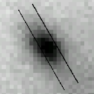
The main problem for observing an appropriate sample of cluster spiral galaxy candidates arises from our restriction to the standard MOS unit of FORS at the time of the observations. Within one setup this mode provides 19 slitlets covering the area of the CCD in y–direction. All of them are individually moveable along the x–axis but have a fixed orientation and therefore a fixed slit angle. Ideally, slits should be placed along the major axis of a galaxy to measure its rotation curve. Since this was impossible for the major fraction of our candidates, we rotated the FORS instrument as to minimize the deviation $\delta$ between slit angle and position angle within one setup. Unavoidably, the deviation $\delta$ was rather large in some cases leading to geometric distortions of the observed velocity profile that could not be fully corrected for.

4 MOS–Observations and data reduction

Observations were carried out in November 1999 (Cl 0413–65), March 2000 (MS 1008–12) and October 2000 (Cl 0303$+$17). Both FORS instruments were mounted at the Cassegrain focus of one of the ESO–VLT unit telescopes, respectively. Each instrument had a 2K Tektronix CCD with 24$\mu$ pixels and was used in the standard mode. This provides a resolution of 0$\aas@@fstack{\prime\prime}$2/pixel with a total FOV of 6$\aas@@fstack{\prime}$8$\times$6$\aas@@fstack{\prime}$8 in imaging mode and a usable FOV of 6$\aas@@fstack{\prime}$8$\times$4$\aas@@fstack{\prime}$0 for MOS.

In total we gained 125 spectra of 116 objects in the range 18.0 $<$ R $<$ 23.0 (some objects were observed within two setups). For each setup a total exposure time in the order of 8000 sec (splitted into 3–5 individual exposures) was chosen to achieve an $S/N\approx 5$ in the emission lines even for the faintest galaxies.

Due to the faintness and the apparent small spatial size of the distant galaxies (in the order of 1″only) particular care has to be taken for placing an object onto a slit. The first order positioning of the slitlets was done on the basis of FORS images and the FIMS–software. After taking a through–slit aquisition frame the final positioning of the slitlets on the targets was within an accuracy of 0$\aas@@fstack{\prime\prime}$1.

We used a slitwidth of 1″and grism GRIS 600R. This provides a resolution of $\lambda/\Delta\lambda=$1230 and a dispersion of 45Å/mm corresponding to a sampling of 1.08 Å/pixel. Each individual spectrum covers typically 2000 Å within a wavelength range between 4400–8200 Å depending on the slit position within the FOV.

Figure 1: Example for the correction of the curvature of the spectra in y–direction. Top. The raw but cosmic corrected two dimensional spectrum of the galaxy A18 (slit no. 18 of setup A) of MS 1008–12 . Center. The same spectrum after applying the rectification. Bottom. The fully reduced and wavelength calibrated spectrum. A18 is an early–type galaxy and a member of MS 1008–12  ($z=0.3111$). Please note that the figures are expanded in y–direction for a better illustration of the curvature.

All data reduction steps were done with MIDAS or with own procedures which were implemented into MIDAS.

Since the ESO–Paranal staff provides calibration frames (as bias, flatfields or standards) of VLT observations in general by following a standard calibration plan we have checked at first all calibration frames for compatibility with their corresponding science frames (e.g. same read–out–mode, sampling, gain etc.). Furthermore, properties of sets of calibration frames contemporary gained with the science frames during one night have been principally compared with other sets e.g. before averaging. In some cases science frames of one setup were collected during several nights. Such sub–setups and their corresponding calibration frames were always treated separately at first to check at which state of the data reduction they could be combined.

Figure 2: Illustration of our observed data by means of one galaxy from Setup B of the cluster MS 1008–12  (ID$=$B5). Left. The spatially resolved $H_{\beta}$–emission line showing clearly the Doppler shifts due to the rotation of the galaxy (for a better illustration the image was expanded in the spatial direction). Center. The corresponding measured rotation curve. Right. Image of the galaxy extracted from the FORS frame. The galaxy with $R=20.70$ has an inclination of 60^∘ and is a cluster member ($z=0.3039$). The slit position is marked.

Firstly, all science and flatfield frames were bias corrected. We created master bias frames for each observing night by the median of typically 20 single bias frames which have been set to the same level before. This was possible since in all cases the mean bias level changed only in the order of $\ll 1$% even between different nights and all frames showed little but equal two dimensional patterns. Then, each master bias was scaled to the overscan level of the science frame and subtracted. Hereafter, a cosmic ray correction on the two dimensional MOS frames has been applied by using the standard MIDAS tool FILTER/COSMIC. Within this routine cosmic ray events are detected by the comparison of the raw frame with a median filtered version of that image. Pixels with an intensity greater than a defined threshold as compared to the local median are replaced by this median value. To avoid misdetections, in particular within the emission lines, we furthermore compared the individual exposures of a given setup.

Now, two dimensional subframes corresponding to individual slit spectra were extracted from each MOS frame. Similarly, appropriate subframes (with same dimensions and CCD–pixel coordinates) were extracted from the corresponding two dimensional flatfield– and calibration images. Flatfields were gained with through–slit–exposures. For each setup two versions with different exposure times were taken to warrant for correct illumination of the upper and lower part of the CCD, respectively. This was necessary to avoid diffuse reflection from the gaps between the slitlets. To perform the correction of the science spectra for pixel–to–pixel variations and the CCD-response over the dispersion direction masterflats were created from typically 3–5 corresponding single flatfields by normalization and averaging.

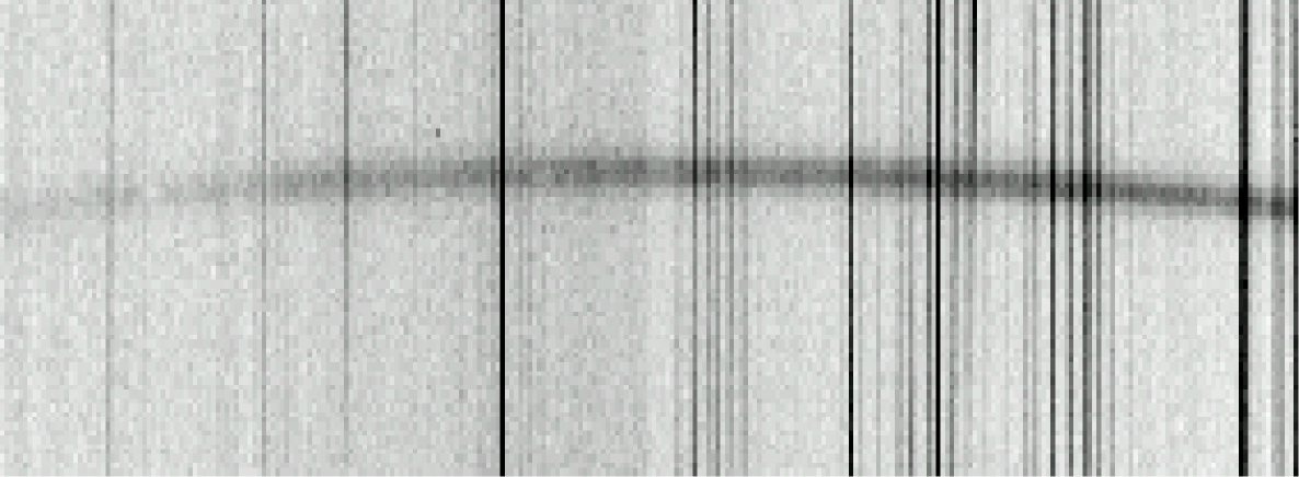
One of the critical steps was the correction for an instrument based curvature of the frames in y–direction (see Fig.1 for an illustration). This distortion changes gradually from a positive curvature at the top of the CCD to a negative curvature at the bottom of the CCD with a maximal misalignment in the order of five pixel (in y) at the edges of the uppermost and lowest spectrum. To correct for, each column of a certain slit image has to be shifted with subpixel accuracy. To get values with a resolution of 0.1 pixel we applied a fit to the curvature. We checked that the flux of the science frames was conserved within a few percent. The same procedure was applied to the calibration spectra. We point out that the rectification for corresponding science/calibration spectra has to be achieved with exactly the same parameters. Furthermore, this reduction step has to be done after the flatfield correction since there are small but non-commutative changes of pixel values which would affect the flatfield correction if doing it in the reverse order.

To subtract the night sky emission typically 30–40 rows
($\approx$ 6″–8″) on both sides of the galaxy emission were selected interactively before each column of a certain spectrum was fitted. Only few galaxy spectra were located very close to the edges of the respective slitlets. In those cases the definition of the sky region was restricted to one side of the galaxy spectrum, only.

Distortions in wavelength direction, i.e. the curvature of arc–lines were corrected during the standard wavelength calibration. Calibration spectra have been taken with Ne, He, and Ar lamps and a two–dimensional dispersion relation (rms $\approx 0.04\AA$) was calculated for each spectrum by polynomial fits. This dispersion relation was then applied to the corresponding science spectrum.

For the summation of single exposures of the same slitlet, the center of the galaxy emission along the spatial axis was determined by a Gaussian fit for each exposure. Only for a very limited number we measured an offset in the order of 1–2 pixel making it necessary to shift along the spatial axis before summation. In the case of seeing variations larger than 25% between individual frames a weighted addition has been applied.

5 Modelling of rotation curves

For the derivation of rotational velocities of the galaxies as a function of radius we followed exactly the same procedure as described in detail in Ziegler et al. (Ziegler2 (2002)) and in Böhm et.al (Boehm (2004)). Both publications present the analysis of the internal kinematics of spiral galaxies at intermediate redshift taken from the FORS Deep Field Survey (e.g. Heidt et al. (JH (2003)). Since these objects were observed with the same instrumental setups as the ones presented here we only summarize the main properties of this part of the analysis.

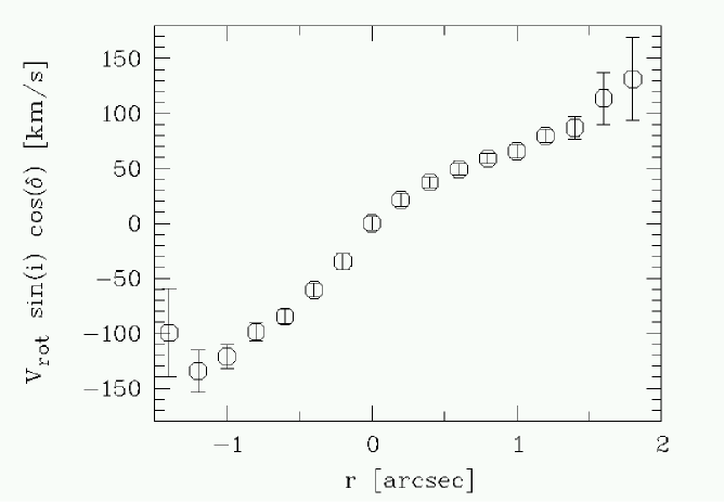
5.1 Observed rotation curve RC_obs

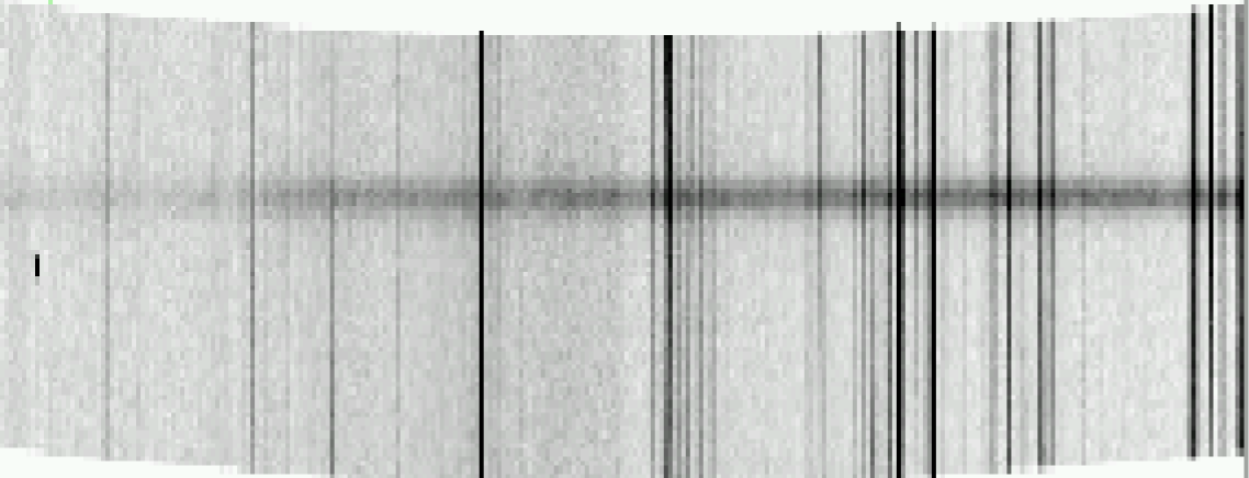
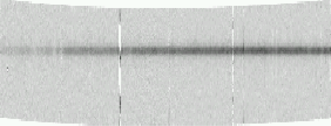
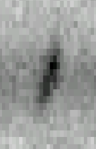
Rotation velocities were determined by an analysis of the [OII] 3727, H_β or [OIII] 5007 emission lines (see Fig.2 for an illustration of our data). Any blue– and redshift in wavelength within an emission line due to the internal kinematics of a galaxy has to be measured with reference to the center of that line. Therefore, we firstly fitted a Gaussian profile to the selected emission line to define its center along the spatial axis within an accuracy of 0$\aas@@fstack{\prime\prime}$1. This was achieved by averaging 100 columns centered on that emission line to construct a one–dimensional intensity profile along the spatial axis.

To determine the wavelength shifts along the spatial axis the emission line was fitted row by row with Gaussian profiles after three neighbouring rows were averaged before each fit to increase the S/N ratio. Due to the resolution of 0$\aas@@fstack{\prime\prime}$2 arcsec/pixel this ”boxcar”–filter corresponds to 0$\aas@@fstack{\prime\prime}$6 (only in the few cases of very weak lines we used a boxcar of 1″). Wavelength shifts relative to the center of the line were now transformed into velocity shifts under consideration of a cosmological correction of $(1+z)^{-1}$ to gain an observed rotation curve RC_obs.

Any velocity value measured on the basis of RC_obs will lead to an underestimation of the true intrinsic maximum galaxy rotation velocity. This is due to the fact that the visible disk size of spirals at intermediate redshifts and the slit width of 1 arcsec are of comparable sizes and, therefore, an integrated spectrum covers a substantial fraction of the two–dimensional intrinsic velocity field of a galaxy. At $z=0.5$ – that is the distance of Cl 0413–65 for example – a typical scalelength of 3kpc corresponds to $\approx$0.5 arcsec. Hence, this ”blurring” effect has to be taken into account in particular for the determination of the maximum rotation velocity V_max. The problem was solved by generating a synthetic rotation curve RC_syn which was compared with RC_obs.

5.2 Synthetic rotation curve RC_syn

To simulate a rotation curve we assumed an intrinsic rotation law. A simple shape was used with a linear rise of V_rot at small radii turning over at a characteristic radius $r_{0}$ into a flat part of V${}_{rot}=const=$V_max as it can be expected due to the influence of a Dark Matter Halo.

Based on RC_syn we generated the two–dimensional velocity field for an individual galaxy as it would appear under consideration of the observed position angle, inclination and disk scale length as determined by a fit to the respective two–dimensional surface brightness profile and the seeing (FWHM) during spectroscopy. Simulating the slit spectroscopy we then integrate over the velocity field within a stripe of 1″taking also into account the mismatch angle $\delta$ to find V_max. This fit was repeated varying the values of $i$, $\delta$ and $r_{d}$ within the errors. For a detailed discussion of a $\chi^{2}$-fitting procedure based on the errors from the RC extraction and a discussion of the influence of different RC_syn shapes on V_max see also Böhm et al. (Boehm (2004)).

In 8 cases more than one emission line was present within a spectrum. Rotation curves have been measured from each line and compared. They were consistent within the errors in 6 cases. The other two had too low S/N. The tabulated values for $V_{max}$ have been derived from the curve with the largest covered radius and the highest S/N ratio.

5.3 Disturbed kinematics of cluster spirals

Only galaxies showing a rotation curve that is rising in the inner region and then turning into a flat part are useful for the construction of a TF–diagram. In such cases the maximum rotation velocity can be used as an indicator for the total dynamical mass of a galaxy and would therefore reflect the influence of a dark matter halo on the internal galaxy kinematics. In Paper I we presented a TF–diagram in which 13 cluster spirals of Cl 0303$+$17 , Cl 0413–65 , and MS 1008–12  as well as seven field spiral galaxies are shown in comparison to the distribution of the FORS Deep Field galaxies from Böhm et al. (Boehm (2004)). We point out that we only used those galaxies for the diagram where we were able to measure V_max in the sense mentioned above. Galaxies with disturbed kinematics (either intrinsic or geometric) do not enter the TF–diagram.

6 The data

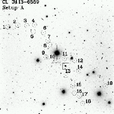
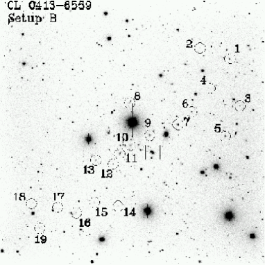
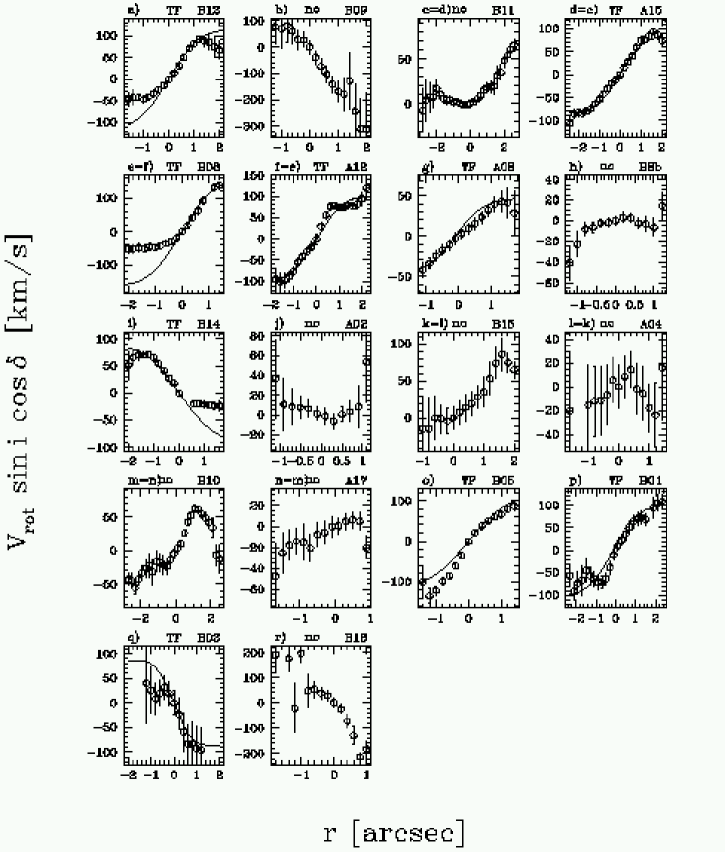
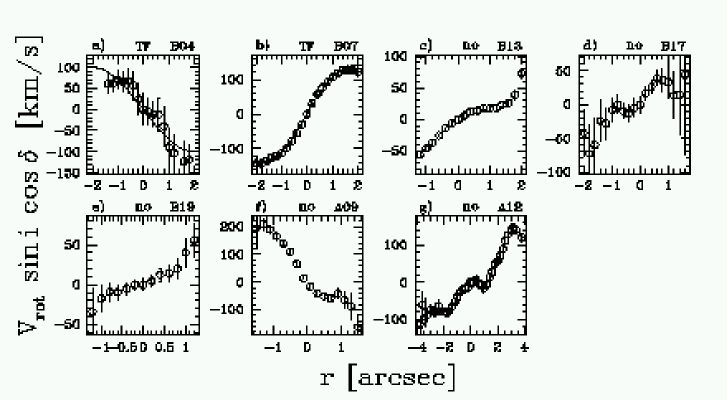
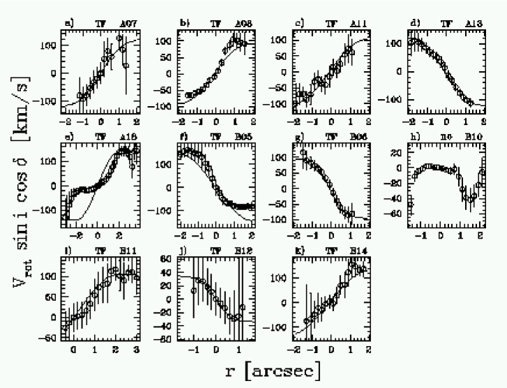
Within this section we present data tables (Table 2–10) on individual galaxies, finding charts (Fig.3) of the six MOS–setups, and position velocity diagrams of galaxies (Fig.4–6) in the field of the clusters.

The finding charts show the full FORS 6$\aas@@fstack{\prime}$8 $\times$ 6$\aas@@fstack{\prime}$8 –FOV in standard imaging mode. All observed primary MOS–targets are marked by circles and labeled by their slit numbers. These numbers correspond to the identifier (ID) given in the data tables. Table 2–4 contain a complete list of all observed objects (within all setups and all slitlets) with positions, redshifts and magnitudes. The positions were measured on our FORS images and are not astrometric corrected.

In Table 5 specific information is given on only those spiral galaxies for which we derived V_max. The columns of that table have the following meaning, respectively:

1. cluster – cluster setup of MOS–spectroscopy.

2. ID — Identification number of galaxies corresponding to the setup (A or B) and the slit number.

3. mem — shows cluster membership of a galaxy.

4. T — type of SED in the de Vaucouleurs scheme. $T=1$ corresponds to Hubble type Sa, $T=3$ to Sb, $T=5$ to Sc, and $T=8$ to Sdm. Classification criteria as described in Böhm et al. (Boehm (2004)).

5. incl.— Disk inclination derived by minimizing $\chi^{2}$ of an exponential profile fit to the galaxy image extracted from our FORS frames.

6. $\delta$ — angle of misalignment between the slit and the apparent major axis of a galaxy.

7. r_d — apparent disk scale length of a galaxy (in arcsec) as derived from ground based data.

8. V_max — Intrinsic maximum rotation velocity of the galaxy (see sect. 5 for details). The Error of the intrinsic maximum rotation velocity was estimated via $\chi^{2}$-fits of the synthetic RC to the observed RC (see Böhm et al. Boehm (2004)).

9. EW [OII] — rest frame equivalent width of the [OII] emission line as derived from our spectra.

10. M_B — Absolute $B$-band magnitude.

In total we gained spectra of 116 objects within the magnitude range 18.0 $<$ R $<$ 23.0. We were able to measure redshifts and to determine spectral types for 89 galaxies. 72 turned out to be late type galaxies. From the 50 galaxies which were found to be cluster members 35 are late type galaxies. Finally, for 32 galaxies (15 cluster members) we were able to obtain position velocity diagrams (Fig.4–6). The corresponding measured values (V_rot versus position) are presented in Tab. 6–10. 13 cluster galaxies exhibit a rotation curve of the universal form rising in the inner region and passing over into a flat part. In those cases (plus 7 field galaxies) V_max could be determined. The other members have peculiar kinematics or too low signal–to–noise.

Figure 3: Finding charts of all MOS setups. Top. MS 1008–12. Center. Cl 0303$+$17. Bottom. Cl 0413–65. In all cases we show the full FORS 6$\aas@@fstack{\prime}$8 $\times$ 6$\aas@@fstack{\prime}$8 –FOV. All primary MOS–targets are marked by circles and labeled by their slit numbers. The central cluster galaxy is marked by a square (north is up, east to the left).

Table 2: MOS targets in the field of MS 1008–12 observed with Setup A (PA$=+55^{\circ}$) and Setup B (PA$=-58^{\circ}$). There are 7 objects which have been observed in both setups: A3$=$B14, A4$=$B15, A6$=$B6, A8$=$B19, A12$=$B8, A15$=$B11 and A17$=$B10. For identification of galaxies see finding chart in Fig.3.

ID	RA	DE	z	V	ID	RA	DE	z	V
	[h m s]	[${\circ}$ ’ ”]		[mag]		[h m s]	[${\circ}$ ’ ”]		[mag]
A1	10 10 23.3	-12 37 27	0.3074		B1	10 10 44.7	-12 36 22	0.3222	20.31
A2	10 10 24.4	-12 37 46	0.3167		B2	10 10 44.1	-12 36 36	0.1673	20.58
A3	10 10 21.8	-12 38 41			B3	10 10 40.5	-12 36 32	0.4256	21.46
A4	10 10 20.6	-12 39 05	0.2960	20.31	B4	10 10 42.8	-12 37 30
A5	10 10 31.9	-12 37 49	0.3090	19.84	B5	10 10 48.0	-12 38 44	0.3039
A6	10 10 37.0	-12 37 15	0.3526	19.98	B6	10 10 37.0	-12 37 15	0.3516	19.98
A7	10 10 37.0	-12 37 51	0.3101	21.45	B7	10 10 33.9	-12 37 21	0.3623	20.63
A8	10 10 22.5	-12 40 54	0.3137	21.13	B8	10 10 42.6	-12 39 10	0.3088	20.76
A9	10 10 29.7	-12 40 06	0.3044	20.76	B9	10 10 29.1	-12 37 36	0.2960	21.02
A10	10 10 29.9	-12 40 18	0.2998	21.52	B10	10 10 46.9	-12 40 33	0.3024	19.78
A11	10 10 42.1	-12 38 56	0.3089	19.64	B11	10 10 42.8	-12 40 22	0.3219	20.14
A12	10 10 42.6	-12 39 10	0.3090	20.76	B12	10 10 36.8	-12 40 06	0.2980	20.78
A13	10 10 38.9	-12 40 18	0.3047	21.61	B13	10 10 32.5	-12 39 54	0.3060	19.54
A14	10 10 45.6	-12 39 42	0.3066	20.58	B14	10 10 21.8	-12 38 41	0.3100
A15	10 10 42.8	-12 40 22	0.3219	20.14	B15	10 10 20.6	-12 39 05	0.2957	20.31
A16	10 10 31.2	-12 42 49	0.3094	20.82	B16	10 10 32.0	-12 41 04	0.4644	21.62
A17	10 10 46.9	-12 40 33	0.3022	19.78	B17	10 10 28.6	-12 41 03	0.3116	20.63
A18	10 10 35.2	-12 43 09	0.3111	20.70	B18	10 10 23.5	-12 40 45		20.80
A19	10 10 37.3	-12 43 08		20.71	B19	10 10 22.5	-12 40 54		21.13
					B7b	10 10 33.7	-12 37 28	0.2983
					B8b	10 10 42.8	-12 39 06	0.3040

Table 3: MOS targets in the field of Cl 0303$+$17 observed with Setup A (PA$=+45^{\circ}$) and Setup B (PA$=-45^{\circ}$). A11$=$B6.

ID	RA	DE	z	R	ID	RA	DE	z	R
	[h m s]	[${\circ}$ ’ ”]		[mag]		[h m s]	[${\circ}$ ’ ”]		[mag]
A1	03 06 05.3	17 22 04	0.5233	21.03	B1	03 06 26.8	17 21 53	0.4232	22.13
A2	03 06 03.0	17 21 12		21.59	B2	03 06 23.6	17 22 13	0.4203	21.01
A3	03 06 05.6	17 21 22	0.4231	21.18	B3	03 06 22.1	17 21 49		21.23
A4	03 06 12.9	17 22 16		21.40	B4	03 06 24.2	17 20 59	0.4237	19.44
A5	03 06 12.9	17 21 50	0.4174	21.83	B5	03 06 18.5	17 21 47		20.97
A6	03 06 11.2	17 20 54	0.4043	21.67	B6	03 06 21.1	17 20 42	0.4142	21.53
A7	03 06 11.4	17 20 35	0.4190	20.81	B7	03 06 21.0	17 20 09	0.3597	19.25
A8	03 06 12.9	17 20 06	0.4207	19.30	B8	03 06 20.7	17 19 51		22.75
A9	03 06 15.1	17 20 21	0.4039	21.11	B9	03 06 18.7	17 19 49	0.4174	21.43
A10	03 06 13.1	17 19 20	0.6413	21.77	B10	03 06 18.2	17 19 12		21.30
A11	03 06 21.1	17 20 42		21.35	B11	03 06 17.8	17 18 45	0.4187	21.42
A12	03 06 22.4	17 20 20	0.1505	19.37	B12	03 06 17.8	17 18 20	0.4169	21.88
A13	03 06 16.7	17 18 25	0.4201	20.68	B13	03 06 08.6	17 19 44	0.1624	20.09
A14	03 06 18.3	17 18 31	0.4209	20.98	B14	03 06 12.3	17 18 25	0.1842	21.42
A15	03 06 20.3	17 18 22	0.4176	21.44	B15	03 06 14.8	17 17 20	0.2453	19.18
A16	03 06 23.4	17 18 35		22.05	B16	03 06 10.7	17 17 55	0.3078	21.68
A17	03 06 24.8	17 18 05	0.4069	21.11	B17	03 06 11.9	17 17 07	0.3095	20.34
A18	03 06 24.8	17 17 48	0.4192	22.85	B18	03 06 05.5	17 17 57		20.91
A19	03 06 23.9	17 17 14		21.69	B19	03 06 09.7	17 16 37	0.5290	22.45
A4b	03 06 12.8	17 22 35	0.4190
A4c	03 06 12.2	17 22 26	0.7463	23.40
A14b	03 06 19.0	17 18 20	0.4171	21.07
A17b	03 06 24.0	17 18 18	0.8060	22.11

Table 4: MOS targets in the field of Cl 0413–65 observed with Setup A (PA$=-45^{\circ}$) and Setup B (PA$=+45^{\circ}$). A11$=$B9.

ID	RA	DE	z	I	ID	RA	DE	z	I
	[h m s]	[${\circ}$ ’ ”]		[mag]		[h m s]	[${\circ}$ ’ ”]		[mag]
A1	04 13 17.6	-65 48 46		21.05	B1	04 12 24.9	-65 48 40	0.5080	20.32
A2	04 13 11.8	-65 48 40		20.60	B2	04 12 32.3	-65 48 24		21.42
A3	04 13 06.6	-65 48 42		20.53	B3	04 12 22.3	-65 49 53		21.19
A4	04 13 02.1	-65 48 39	0.6537	20.64	B4	04 12 29.7	-65 49 26	0.5525	22.31
A5	04 13 02.8	-65 49 02		22.19	B5	04 12 25.9	-65 50 40	0.6066	20.20
A6	04 12 57.0	-65 49 06		21.00	B6	04 12 34.3	-65 50 02	0.5082	20.99
A7	04 12 54.5	-65 49 35	0.5644	20.78	B7	04 12 37.8	-65 50 21		19.87
A8	04 12 53.4	-65 49 48	0.4989	21.59	B8	04 12 50.0	-65 49 49	0.6260	21.05
A9	04 12 55.6	-65 50 33	0.8017	20.94	B9	04 12 44.9	-65 50 38	0.5395	19.68
A10	04 12 49.7	-65 50 45		21.04	B10	04 12 49.4	-65 50 52	0.1847	20.61
A11	04 12 44.9	-65 50 38	0.5395	19.68	B11	04 12 52.4	-65 51 07	0.5099	19.92
A12	04 12 40.8	-65 50 37		21.67	B12	04 12 54.0	-65 51 23	0.5103	21.15
A13	04 12 44.1	-65 51 37	0.6067	21.01	B13	04 12 58.3	-65 51 16	0.5082	20.39
A14	04 12 36.8	-65 51 23	0.5391	19.86	B14	04 12 52.9	-65 52 27	0.5097	21.47
A15	04 12 40.2	-65 52 14	0.5423	20.07	B15	04 12 58.7	-65 52 22	0.6186	21.22
A16	04 12 39.3	-65 52 40		20.58	B16	04 13 03.3	-65 52 38
A17	04 12 36.3	-65 52 51	0.5381	20.85	B17	04 13 08.0	-65 52 29	0.8479	22.00
A18	04 12 34.4	-65 53 17	0.6082	20.87	B18	04 13 14.7	-65 52 23		21.79
A19	04 12 21.4	-65 52 15		20.08	B19	04 13 12.5	-65 53 02		21.40
A9b	04 12 55.2	-65 50 35	0.4254	19.18	B8b	04 12 49.7	-65 49 46		21.71
A12b	04 12 40.8	-65 50 36	0.0853	16.70	B10b	04 12 49.4	-65 50 52	0.5035	21.19
A17b	04 12 35.8	-65 52 54	0.5062	21.38

Table 5: All galaxies from which we obtained V_max. In the case of MS 1008–12 A12$=$B8. For an identification see finding charts in fig. 3. In some cases there was no [OII] line within the spectra and we used other emission lines.

cluster	ID	mem	Type	incl.	$\delta$	rd	Vmax	EW ([OII])	MB
				[deg]	[deg]	[”]	[km/s]	[Å]	[mag]
(1)	(2)	(3)	(4)	(5)	(6)	(7)	(8)	(9)	(10)
MS 1008–12	A8	yes	+8	45	5	0.40	70$\pm$30	72.8	-20.19
MS 1008–12	A12	yes	+5	50	43	0.70	220$\pm$59		-20.69
MS 1008–12	A15	yes	+5	20	20	0.57	270$\pm$126		-21.24
MS 1008–12	B1	yes	+5	60	-9	1.35	130$\pm$23		-20.15
MS 1008–12	B3	no	+1	55	63	0.40	320$\pm$129	5.1	-21.26
MS 1008–12	B5	yes	+5	60	10	0.60	150$\pm$26		-20.32
MS 1008–12	B8	yes	+5	50	-17	0.70	240$\pm$49		-20.69
MS 1008–12	B12	yes	+5	50	8	0.60	160$\pm$32		-20.52
MS 1008–12	B14	yes	+5	52	-50	1.02	230$\pm$68	15.7	-21.48
Cl 0303$+$17	B4	yes	+3	20	-30	0.80	400$\pm$135	5.1	-22.13
Cl 0303$+$17	B7	no	+5	35	25	0.72	320$\pm$62	19.4	-21.98
Cl 0413–65	A7	no	+3	54	19	0.45	200$\pm$26	12.3	-20.94
Cl 0413–65	A8	yes	+8	65	-20	0.60	150$\pm$18	39.5	-20.12
Cl 0413–65	A11	no	+3	33	0	0.85	350$\pm$96	10.3	-21.65
Cl 0413–65	A13	no	+5	50	25	0.55	202$\pm$29	14.1	-21.16
Cl 0413–65	A18	no	+5	60	20	0.80	205$\pm$38	36.1	-21.30
Cl 0413–65	B5	no	+5	35	-5	0.95	300$\pm$79	25.3	-21.53
Cl 0413–65	B6	yes	+5	40	-15	0.25	165$\pm$27	17.1	-20.41
Cl 0413–65	B11	yes	+3	55	15	0.52	180$\pm$23	11.4	-21.52
Cl 0413–65	B12	yes	+5	43	-75	0.30	230$\pm$130	7.2	-20.42
Cl 0413–65	B14	yes	+3	63	-22	0.40	220$\pm$27	4.5	-20.00

Figure 4: Position velocity diagrams of galaxies in the field of MS 1008–12. Galaxies which entered the TF diagram presented in Paper I are labeled (TF). The solid line represents the projected best fitting model profile. See Table 6–8 for comparison.

Figure 5: Position velocity diagrams of galaxies in the field of Cl 0303$+$17. Galaxies which entered the TF diagram presented in Paper I are labeled (TF). The solid line represents the projected best fitting model profile. See Table 9 for comparison.

Figure 6: Position velocity diagrams of galaxies in the field of Cl 0413–65. Galaxies which entered the TF diagram presented in Paper I are labeled (TF). The solid line represents the projected best fitting model profile. See Table 10 and 11 for comparison.

Table 6: Measured rotation velocities V_rot as function of projected distance (Pos) to the galaxies’ centers (Pos$=$0) for MS 1008–12. Galaxies are indicated by their ID with the measured emission line, respectively. See Fig.4 for comparison.

Pos	Vrot sin $i$ cos $\delta$
[”]	[km s-1]
	B12(Hβ)	B9(O[II])	B11(Hβ)	A15(O[III])	B8(Hβ)	A12(O[III])	B8b(O[III])	B14(Hβ)
-2.8			-7.1$\pm$24.0
-2.6			+4.3$\pm$23.3
-2.4			+7.7$\pm$16.8	-107.2$\pm$19.1
-2.2			+7.8$\pm$12.3	-85.1$\pm$9.8
-2.0			+17.4$\pm$9.5	-82.6$\pm$8.3	-51.3$\pm$13.8			+50.3$\pm$25.1
-1.8			+11.1$\pm$5.9	-85.2$\pm$7.3	-51.3$\pm$14.3	-95.7$\pm$26.5		+65.2$\pm$13.2
-1.6	-47.3$\pm$16.0		+6.0$\pm$5.2	-79.7$\pm$5.5	-48.3$\pm$13.7	-100.1$\pm$17.9		+69.5$\pm$8.6
-1.4	-42.7$\pm$16.4		+4.3$\pm$4.5	-74.4$\pm$5.6	-51.3$\pm$11.2	-97.8$\pm$16.4		+69.6$\pm$5.6
-1.2	-42.7$\pm$7.9	+76.6$\pm$64.4	+4.2$\pm$4.2	-64.1$\pm$6.1	-45.4$\pm$10.7	-88.0$\pm$12.7	-40.8$\pm$16.6	+71.1$\pm$3.3
-1.0	-47.6$\pm$7.1	+69.4$\pm$75.5	+2.1$\pm$3.8	-54.9$\pm$6.1	-46.7$\pm$9.1	-76.2$\pm$10.7	-22.8$\pm$12.0	+65.6$\pm$4.4
-0.8	-40.9$\pm$6.2	+80.8$\pm$61.0	+2.1$\pm$3.5	-42.8$\pm$6.4	-43.2$\pm$8.1	-55.8$\pm$10.1	-8.1$\pm$6.8	+53.3$\pm$5.1
-0.6	-33.6$\pm$5.3	+59.5$\pm$48.4	+0.8$\pm$2.9	-30.4$\pm$5.9	-36.4$\pm$8.0	-42.2$\pm$8.4	-6.4$\pm$5.4	+41.5$\pm$5.5
-0.4	-24.7$\pm$4.5	+28.5$\pm$35.9	-0.4$\pm$2.5	-18.7$\pm$5.8	-29.1$\pm$7.8	-30.1$\pm$9.6	-2.3$\pm$4.0	+27.4$\pm$5.9
-0.2	-13.8$\pm$4.3	+27.6$\pm$27.9	-0.4$\pm$2.3	-12.2$\pm$4.7	-18.8$\pm$7.5	-18.8$\pm$10.4	-1.6$\pm$3.8	+17.6$\pm$5.5
+0.0	+0.0$\pm$4.2	+0.0$\pm$26.6	+0.0$\pm$2.2	+0.0$\pm$4.7	+0.0$\pm$8.0	+0.0$\pm$12.2	+0.0$\pm$4.4	+0.0$\pm$5.2
+0.2	+14.1$\pm$4.1	-39.2$\pm$25.0	+1.9$\pm$2.4	+14.9$\pm$6.6	+18.3$\pm$8.9	+29.0$\pm$11.1	+3.3$\pm$4.8
+0.4	+29.9$\pm$4.0	-73.9$\pm$28.0	+5.5$\pm$2.8	+27.8$\pm$6.8	+41.5$\pm$9.6	+55.8$\pm$9.2	+2.3$\pm$4.4
+0.6	+49.9$\pm$5.0	-103.3$\pm$30.2	+9.2$\pm$4.1	+40.5$\pm$6.9	+62.6$\pm$11.2	+75.7$\pm$6.7	-2.4$\pm$5.3	-20.7$\pm$3.4
+0.8	+69.7$\pm$6.2	-141.0$\pm$30.7	+15.7$\pm$5.0	+59.7$\pm$8.4	+92.3$\pm$10.4	+78.7$\pm$5.2	-3.2$\pm$6.8	-19.0$\pm$3.8
+1.0	+81.9$\pm$5.5	-168.5$\pm$41.4	+18.2$\pm$5.9	+75.2$\pm$8.5	+132.3$\pm$12.9	+74.1$\pm$4.8	-6.5$\pm$8.6	-21.2$\pm$3.8
+1.2	+92.5$\pm$6.0	-179.7$\pm$64.9	+18.9$\pm$6.8	+77.4$\pm$8.0	+138.3$\pm$11.7	+74.9$\pm$5.0	+14.3$\pm$13.0	-21.7$\pm$4.5
+1.4	+87.4$\pm$11.4	-127.2$\pm$108.3	+19.8$\pm$8.8	+84.9$\pm$7.2		+79.4$\pm$6.1		-23.8$\pm$5.9
+1.6	+85.8$\pm$19.5	-244.6$\pm$102.0	+32.1$\pm$9.7	+93.8$\pm$6.8		+76.6$\pm$6.9		-23.9$\pm$10.3
+1.8	+73.7$\pm$24.3	-312.3$\pm$112.9	+35.3$\pm$8.2	+87.3$\pm$9.1		+81.2$\pm$10.7
+2.0	+67.3$\pm$21.5	-313.4$\pm$137.8	+48.3$\pm$6.8	+74.5$\pm$12.1		+93.7$\pm$16.3
+2.2			+54.6$\pm$5.1			+120.6$\pm$29.0
+2.4			+61.3$\pm$5.4
+2.6			+65.9$\pm$6.6

———————————————————————————————————————————————

Table 7: Measured rotation velocities V_rot as function of projected distance (Pos) to the galaxies’ centers (Pos$=$0) for MS 1008–12. Galaxies are indicated by their ID with the measured emission line, respectively. See Fig.4 for comparison.

Pos	Vrot sin $i$ cos $\delta$
[”]	[km s-1]
	B15(O[II])	A4(O[II])	B5(Hβ)	B3(O[II])	B16(O[II])
-1.8					+191.4$\pm$72.2
-1.6		-20.4$\pm$49.4
-1.4			-99.6$\pm$40.2		+175.7$\pm$51.8
-1.2			-134.5$\pm$19.1	+39.9$\pm$80.4	-21.0$\pm$98.0
-1.0	-14.3$\pm$41.3	-15.5$\pm$33.8	-121.1$\pm$10.8	+25.9$\pm$47.2	+197.0$\pm$34.2
-0.8	-14.1$\pm$41.9	-12.2$\pm$29.4	-98.8$\pm$8.3	+8.1$\pm$32.4	+47.5$\pm$66.0
-0.6	+0.1$\pm$28.7	-11.6$\pm$28.4	-84.7$\pm$6.3	+19.6$\pm$26.3	+52.7$\pm$33.4
-0.4	-1.4$\pm$19.6	-6.9$\pm$25.3	-60.6$\pm$6.5	+30.9$\pm$24.6	+37.6$\pm$24.7
-0.2	-4.4$\pm$16.9	+5.6$\pm$18.5	-34.7$\pm$7.7	+17.8$\pm$24.5	+28.5$\pm$21.5
+0.0	+0.0$\pm$15.4	+0.0$\pm$18.3	+0.0$\pm$6.3	+0.0$\pm$24.0	+0.0$\pm$18.8
+0.2	+7.6$\pm$16.4	+8.3$\pm$17.2	+21.4$\pm$6.4	-23.0$\pm$31.6	-24.6$\pm$17.4
+0.4	+14.0$\pm$17.8	+14.3$\pm$14.7	+37.3$\pm$5.1	-58.8$\pm$38.8	-72.4$\pm$27.3
+0.6	+19.7$\pm$15.6	-1.9$\pm$21.6	+49.3$\pm$5.1	-83.6$\pm$40.0	-129.0$\pm$37.2
+0.8	+28.2$\pm$14.7	-5.8$\pm$22.3	+59.1$\pm$4.3	-83.4$\pm$43.4	-214.7$\pm$16.1
+1.0	+35.2$\pm$20.4	-18.0$\pm$20.6	+65.8$\pm$6.1	-93.0$\pm$46.0	-183.8$\pm$29.6
+1.2	+53.2$\pm$22.4	-24.0$\pm$26.8	+79.5$\pm$6.5	-95.4$\pm$44.7
+1.4	+73.6$\pm$21.3	+16.1$\pm$43.9	+87.0$\pm$10.2
+1.6	+85.8$\pm$22.4
+1.8	+74.4$\pm$12.8
+2.0	+64.9$\pm$11.0

Table 8: Measured rotation velocities V_rot as function of projected distance (Pos) to the galaxies’ centers (Pos$=$0) for MS 1008–12. Galaxies are indicated by their ID with the measured emission line, respectively. See Fig.4 for comparison.

Pos	Vrot sin $i$ cos $\delta$
[”]	[km s-1]
	A8(O[II])	A2(O[III])	B10(Hβ)	A17(O[III])	B1(Hβ)
-2.7			-43.2$\pm$+9.3
-2.5			-45.1$\pm$11.7
-2.3			-55.8$\pm$8.7		-57.7$\pm$24.2
-2.1			-43.3$\pm$7.1		-91.7$\pm$19.4
-1.9			-33.3$\pm$10.0		-74.0$\pm$24.9
-1.7			-26.2$\pm$13.1	-47.6$\pm$31.0	-67.5$\pm$33.1
-1.5			-22.5$\pm$17.9	-25.1$\pm$18.9	-45.4$\pm$27.3
-1.3			-32.0$\pm$19.1	-17.6$\pm$14.1	-57.4$\pm$20.5
-1.1	-42.1$\pm$8.4	+36.6$\pm$40.1	-16.6$\pm$15.5	-13.9$\pm$11.7	-63.4$\pm$16.7
-0.9	-34.0$\pm$6.7	+10.7$\pm$25.7	-17.4$\pm$13.3	-14.9$\pm$17.1	-72.0$\pm$15.9
-0.7	-24.6$\pm$6.6	+8.1$\pm$18.3	-21.5$\pm$14.7	-20.4$\pm$13.3	-71.4$\pm$14.2
-0.5	-17.4$\pm$6.2	+7.5$\pm$11.3	-23.8$\pm$13.1	-7.8$\pm$11.2	-64.3$\pm$13.7
-0.3	-10.8$\pm$6.6	+6.2$\pm$9.0	-12.8$\pm$10.7	-5.6$\pm$ 9.9	-39.1$\pm$14.5
-0.1	-3.2$\pm$6.7	+1.4$\pm$7.1	-4.0$\pm$6.3	-0.2$\pm$ 9.4	-10.2$\pm$12.9
+0.1	+3.2$\pm$6.7	-1.4$\pm$8.1	+4.0$\pm$5.3	+0.2$\pm$ 7.7	+10.2$\pm$11.4
+0.3	+9.4$\pm$6.7	-6.4$\pm$7.2	+10.4$\pm$4.7	+4.5$\pm$ 7.7	+22.8$\pm$12.0
+0.5	+15.6$\pm$7.3	+0.5$\pm$7.3	+26.5$\pm$4.6	+6.1$\pm$ 8.0	+35.1$\pm$13.2
+0.7	+23.7$\pm$7.4	+3.3$\pm$10.6	+42.1$\pm$5.3	+4.9$\pm$ 8.6	+51.2$\pm$13.3
+0.9	+32.2$\pm$8.1	+8.3$\pm$21.4	+52.0$\pm$5.4	-19.8$\pm$ 10.9	+63.6$\pm$14.5
+1.1	+39.5$\pm$9.6	+54.0$\pm$41.2	+62.7$\pm$5.2		+69.1$\pm$14.6
+1.3	+43.0$\pm$13.0		+60.9$\pm$6.3		+71.2$\pm$14.8
+1.5	+41.3$\pm$18.3		+54.8$\pm$5.6		+67.9$\pm$12.9
+1.7	+28.9$\pm$27.2		+49.1$\pm$7.5
+1.9			+42.3$\pm$8.2		+94.2$\pm$22.0
+2.1			+34.2$\pm$14.1		+105.1$\pm$19.2
+2.3			-6.6$\pm$15.3		+106.8$\pm$16.0
+2.5			-12.5$\pm$21.2

———————————————————————-

Table 9: Measured rotation velocities V_rot as function of projected distance (Pos) to the galaxies’ centers (Pos$=$0) for Cl 0303$+$17. Galaxies are indicated by their ID with the measured emission line, respectively. See Fig.5 for comparison.

Pos	Vrot sin $i$ cos $\delta$						Pos	Vrot sin $i$ cos $\delta$
[”]	[km s-1]						[”]	[km s-1]
	B4(O[III])	B7(O[II])	B13(O[III])	B17(Hβ)	B19(O[II])	A12(O[III])		A9(O[II])
-3.8						-112.9$\pm$21.8
-3.6						-60.1$\pm$36.2
-3.4						-80.9$\pm$37.3
-3.2						-87.4$\pm$18.2
-3.0						-74.0$\pm$14.1
-2.8						-78.7$\pm$14.6
-2.6						-79.0$\pm$14.5
-2.4						-63.5$\pm$16.0
-2.2						-78.2$\pm$8.9
-2.0		-142.9$\pm$19.3		-42.2$\pm$33.1		-79.0$\pm$8.5
-1.8		-143.2$\pm$13.4		-72.7$\pm$42.3		-82.9$\pm$7.6
-1.6		-136.1$\pm$9.3		-59.7$\pm$39.8		-76.8$\pm$8.1	-1.5	+195.$\pm$71.3
-1.4	+60.7$\pm$23.7	-126.4$\pm$7.8		-23.9$\pm$31.2		-66.4$\pm$9.3	-1.3	+208.$\pm$22.4
-1.2	+60.7$\pm$20.5	-120.5$\pm$6.8	-56.6$\pm$3.3	-28.1$\pm$23.7	-33.9$\pm$28.5	-52.7$\pm$10.3	-1.1	+190.$\pm$12.9
-1.0	+69.6$\pm$21.4	-113.9$\pm$6.3	-46.3$\pm$2.8	-8.0$\pm$16.9	-17.3$\pm$16.4	-39.6$\pm$11.6	-0.9	+165.$\pm$10.8
-0.8	+65.8$\pm$23.8	-98.7$\pm$6.0	-37.0$\pm$2.3	-0.2$\pm$13.3	-9.0$\pm$11.5	-25.3$\pm$11.6	-0.7	+140.$\pm$11.4
-0.6	+67.1$\pm$29.6	-78.2$\pm$5.0	-25.5$\pm$1.7	-9.7$\pm$10.4	-9.7$\pm$9.7	-20.9$\pm$11.9	-0.5	+109.$\pm$9.3
-0.4	+56.5$\pm$34.1	-55.1$\pm$4.3	-14.1$\pm$1.4	-13.4$\pm$12.1	-5.4$\pm$7.9	-16.6$\pm$12.2	-0.3	+65.$\pm$5.4
-0.2	+24.4$\pm$35.4	-29.3$\pm$5.0	-6.1$\pm$1.9	-4.8$\pm$13.0	-0.3$\pm$6.9	-12.5$\pm$13.2	-0.1	+15.$\pm$4.8
+0.0	+0.0$\pm$36.3	+0.0$\pm$5.8	+0.0$\pm$2.5	+0.0$\pm$11.8	+0.0$\pm$7.0	+0.0$\pm$11.8	+0.1	-15.$\pm$5.0
+0.2	-6.3$\pm$30.8	+30.8$\pm$5.8	+5.9$\pm$3.0	+17.3$\pm$9.6	+4.5$\pm$7.1	+1.1$\pm$11.6	+0.3	-40.$\pm$4.9
+0.4	-11.2$\pm$28.2	+57.6$\pm$5.5	+11.5$\pm$2.8	+26.1$\pm$10.1	+12.0$\pm$8.4	+5.3$\pm$12.6	+0.5	-51.$\pm$5.7
+0.6	-12.2$\pm$39.9	+76.5$\pm$6.2	+13.9$\pm$3.1	+39.1$\pm$11.1	+14.6$\pm$10.4	-5.2$\pm$10.7	+0.7	-59.$\pm$7.5
+0.8	-38.9$\pm$46.9	+93.3$\pm$8.1	+18.0$\pm$3.4	+36.1$\pm$16.0	+19.7$\pm$12.7	-7.4$\pm$12.0	+1.9	-41.$\pm$17.8
+1.0	-89.3$\pm$45.7	+106.0$\pm$9.0	+17.5$\pm$3.6	+33.5$\pm$25.3	+39.9$\pm$17.0	-15.5$\pm$12.4	+1.1	-64.$\pm$31.8
+1.2	-103.9$\pm$43.2	+117.7$\pm$8.6	+18.6$\pm$3.6	+13.1$\pm$34.1	+56.0$\pm$20.7	-6.1$\pm$13.1	+1.3	-87.$\pm$46.2
+1.4		+127.3$\pm$7.1	+24.1$\pm$4.3	+14.7$\pm$59.4		+13.3$\pm$11.9	+1.5	-163.$\pm$44.5
+1.6	-122.5$\pm$48.8	+129.2$\pm$8.5	+26.3$\pm$5.7	+43.8$\pm$118.0		+27.5$\pm$12.5
+1.8	-119.3$\pm$37.5	+126.0$\pm$10.8	+39.6$\pm$7.9			+48.8$\pm$12.4
+2.0		+122.4$\pm$14.0	+72.9$\pm$7.3			+56.7$\pm$13.0
+2.2						+72.0$\pm$13.1
+2.4						+89.3$\pm$13.7
+2.6						+112.1$\pm$13.6
+2.8						+128.6$\pm$11.4
+3.0						+139.5$\pm$9.2
+3.2						+147.8$\pm$7.6
+3.4						+141.2$\pm$8.5
+3.6
+3.8						+120.5$\pm$11.0

Table 10: Measured rotation velocities V_rot as function of projected distance (Pos) to the galaxies’ centers (Pos$=$0) for Cl 0413–65. Galaxies are indicated by their ID with the measured emission line, respectively. See Fig.6 for comparison.

Pos	Vrot sin $i$ cos $\delta$
[”]	[km s-1]
	A7(O[II])	A18(O[II])	B5(O[II])	B11(O[II])	B12(O[II])
-3.0		-130.3$\pm$80.2
-2.8		-115.7$\pm$75.9
-2.6		-78.4$\pm$55.3
-2.4		-51.2$\pm$35.9
-2.2		-31.6$\pm$23.0
-2.0		-26.3$\pm$15.1	+142.9$\pm$19.7
-1.8		-17.6$\pm$10.5	+156.5$\pm$21.8
-1.6		-14.8$\pm$8.5	+161.6$\pm$26.0
-1.4		-15.2$\pm$8.4	+159.4$\pm$31.6
-1.2	-79.2$\pm$64.7	-16.3$\pm$8.8	+150.4$\pm$33.3
-1.0	-93.0$\pm$44.9	-18.1$\pm$8.8	+145.4$\pm$39.3		+12.7$\pm$39.7
-0.8	-79.5$\pm$38.3	-16.3$\pm$9.5	+130.6$\pm$46.7		+28.1$\pm$36.5
-0.6	-53.7$\pm$38.7	-13.1$\pm$10.5	+104.4$\pm$38.3		+26.7$\pm$30.1
-0.4	-32.6$\pm$39.8	-11.7$\pm$11.0	+82.8$\pm$31.4	-25.9$\pm$38.3	+18.4$\pm$26.1
-0.2	-18.1$\pm$37.5	-6.9$\pm$11.3	+39.1$\pm$35.0	-13.1$\pm$36.7	+11.2$\pm$26.3
+0.0	+0.0$\pm$39.1	+0.0$\pm$11.5	+0.0$\pm$32.4	+0.0$\pm$34.2	+0.0$\pm$23.8
+0.2	+50.9$\pm$62.4	+7.2$\pm$11.1	-22.4$\pm$26.5	+3.6$\pm$33.7	-6.1$\pm$21.9
+0.4	+78.9$\pm$48.0	+14.9$\pm$11.8	-50.9$\pm$22.0	+5.6$\pm$31.4	-13.0$\pm$22.9
+0.6	+58.7$\pm$45.3	+19.9$\pm$12.9	-64.9$\pm$15.2	+16.3$\pm$32.7	-25.2$\pm$26.7
+0.8		+27.6$\pm$14.7	-70.8$\pm$12.2	+33.2$\pm$36.0	-29.5$\pm$41.9
+1.0	+125.3$\pm$39.6	+42.3$\pm$16.5	-78.0$\pm$9.6	+54.6$\pm$39.1	-25.3$\pm$86.9
+1.2	+84.5$\pm$53.7	+60.5$\pm$18.1	-82.8$\pm$9.4	+73.3$\pm$38.5	-12.5$\pm$166.9
+1.4	+26.9$\pm$102.3	+78.1$\pm$20.1	-83.6$\pm$10.3	+79.7$\pm$42.8
+1.6		+97.2$\pm$21.7	-84.8$\pm$11.2	+83.1$\pm$46.9
+1.8		+122.5$\pm$21.5	-82.0$\pm$12.7	+112.9$\pm$27.9
+2.0		+139.5$\pm$19.8	-81.6$\pm$15.5	+117.5$\pm$26.3
+2.2		+142.4$\pm$17.9		+101.7$\pm$38.0
+2.4		+142.5$\pm$17.9		+90.2$\pm$44.0
+2.6		+145.2$\pm$19.0		+109.1$\pm$19.1
+2.8		+141.2$\pm$20.6		+110.4$\pm$24.6
+3.0		+120.5$\pm$28.0		+97.5$\pm$40.2
+3.2		+78.4$\pm$44.1
+3.4		+141.8$\pm$33.5
+3.6		+143.5$\pm$54.8

Table 11: Measured rotation velocities V_rot as function of projected distance (Pos) to the galaxies’ centers (Pos$=$0) for Cl 0413–65. Galaxies are indicated by their ID with the measured emission line, respectively. See Fig.6 for comparison.

Pos	Vrot sin $i$ cos $\delta$
[”]	[km s-1]
	A8(O[II])	A11(O[III])	A13(O[II])	B6(O[II])	B10(O[III])	B14(O[II])
-1.9		-98.2$\pm$60.3	+102.2$\pm$46.5
-1.7		-69.9$\pm$33.1	+112.5$\pm$39.3
-1.5	-65.4$\pm$7.2	-68.4$\pm$22.5	+104.7$\pm$30.9	+114.7$\pm$51.1	-48.1$\pm$12.9
-1.3	-65.5$\pm$4.1	-87.1$\pm$24.3	+96.3$\pm$22.3	+89.1$\pm$29.2	-11.0$\pm$6.3	-75.5$\pm$146.5
-1.1	-57.7$\pm$3.9	-70.9$\pm$30.0	+84.5$\pm$18.3	+82.4$\pm$19.6	-4.4$\pm$4.0	-66.3$\pm$103.3
-0.9	-53.4$\pm$3.9	-30.7$\pm$28.3	+70.8$\pm$16.0	+73.3$\pm$15.3	-1.0$\pm$2.7	-48.8$\pm$56.0
-0.7	-46.4$\pm$4.0	-22.2$\pm$24.4	+61.1$\pm$17.2	+62.8$\pm$12.1	+1.9$\pm$2.0	-20.8$\pm$60.2
-0.5	-34.5$\pm$4.2	-37.9$\pm$24.4	+50.7$\pm$18.3	+52.4$\pm$10.4	+2.3$\pm$1.8	-30.2$\pm$47.2
-0.3	-17.6$\pm$4.3	-40.6$\pm$28.3	+34.9$\pm$17.6	+33.2$\pm$11.0	+0.8$\pm$1.6	-6.2$\pm$28.8
-0.1	-8.6$\pm$4.8	-15.0$\pm$32.2	+13.9$\pm$17.4	+12.8$\pm$13.1	+0.3$\pm$1.7	+3.5$\pm$26.0
+0.1	+8.6$\pm$5.4	+15.0$\pm$26.3	-13.9$\pm$15.9	-12.8$\pm$13.3	-0.3$\pm$1.9	-3.5$\pm$29.6
+0.3	+34.3$\pm$9.4	+3.8$\pm$23.5	-32.1$\pm$13.3	-38.8$\pm$15.5	-3.0$\pm$2.7	+28.0$\pm$33.8
+0.5	+70.3$\pm$10.2	+25.2$\pm$23.5	-55.3$\pm$11.8	-60.6$\pm$17.1	-4.0$\pm$3.9	+69.8$\pm$37.8
+0.7	+86.6$\pm$14.9	+53.9$\pm$33.3	-76.8$\pm$11.7	-76.9$\pm$19.7	-1.7$\pm$7.0	+73.2$\pm$52.3
+0.9	+104.3$\pm$18.6	+72.6$\pm$44.1	-91.5$\pm$12.4	-84.9$\pm$24.1	-11.2$\pm$12.1	+122.6$\pm$54.3
+1.1	+101.9$\pm$22.2	+62.4$\pm$40.3	-103.2$\pm$11.2	-80.1$\pm$33.9	-27.6$\pm$15.1	+155.1$\pm$51.6
+1.3	+96.1$\pm$26.9		-111.8$\pm$13.4		-39.1$\pm$15.5	+146.1$\pm$39.9
+1.5	+92.3$\pm$32.7				-41.7$\pm$15.5	+131.9$\pm$21.1
+1.7					-36.4$\pm$14.0	+136.7$\pm$30.9
+1.9					-22.0$\pm$15.7
+2.1					-5.6$\pm$18.9