Primordial non-Gaussianity: local curvature method and statistical significance of constraints on $f_{\rm NL}$ from WMAP data

Abstract

We test the consistency of estimates of the non-linear coupling constant $f_{\rm NL}$ using non-Gaussian CMB maps generated by the method described in (Liguori, Matarrese and Moscardini 2003). This procedure to obtain non-Gaussian maps differs significantly from the method used in previous works on estimation of $f_{\rm NL}$. Nevertheless, using spherical wavelets, we find results in very good agreement with (Mukherjee and Wang 2004), showing that the two ways of generating primordial non-Gaussian maps give equivalent results. Moreover, we introduce a new method for estimating the non-linear coupling constant from CMB observations by using the local curvature of the temperature fluctuation field. We present both Bayesian credible regions (assuming a flat prior) and proper (frequentist) confidence intervals on $f_{\rm NL}$, and discuss the relation between the two approaches. The Bayesian approach tends to yield lower error bars than the frequentist approach, suggesting that a careful analysis of the different interpretations is needed. Using this method, we estimate $f_{\rm NL}=-10^{+270}_{-260}$ at the $2\sigma$ level (Bayesian) and $f_{\rm NL}=-10^{+310}_{-270}$ (frequentist). Moreover, we find that the wavelet and the local curvature approaches, which provide similar error bars, yield approximately uncorrelated estimates of $f_{NL}$ and therefore, as advocated in (Cabella et al. 2004), the estimates may be combined to reduce the error bars. In this way, we obtain $f_{NL}=-5\pm 85$ and $f_{NL}=-5\pm 175$ at the $1\sigma$ and $2\sigma$ level respectively using the frequentist approach.

1 Introduction

Inflation is the standard paradigm for providing the initial conditions for structure formation and Cosmic Microwave Background (CMB) anisotropy generation. In the inflationary picture, primordial adiabatic perturbations arise from quantum fluctuations of the inflaton scalar field which drives the accelerated Universe expansion. In the simplest models, the inflaton is assumed to have a shallow potential, thereby leading to a slow rolling of this field down its potential. The flatness of the potential implies that intrinsic non-linear (hence non-Gaussian) effects during slow-roll inflation are tiny, although non-zero and calculable [Falk, Rangarajan & Srednicki 1993, Gangui et al. 1994, Lesgourgues, Polarski & Starobinsky 1997, Wang & Kamionkowski 2000, Acquaviva et al. 2003, Maldacena 2002]. To quantitatively describe the theoretical findings in this framework, let us introduce a useful parameterisation of non-Gaussianity according to which the primordial gravitational potential $\Phi$ is given by a linear Gaussian term $\phi_{\rm G}$, plus a quadratic contribution, as follows (e.g. [Verde et al. 2000]):

$$\Phi({\bf x})=\phi_{\rm G}({\bf x})+f_{\rm NL}\phi_{\rm G}^{2}({\bf x})$$ (1)

(up to a constant offset, which only affects the monopole contribution), where the dimensionless parameter $f_{\rm NL}$ sets the strength of non-Gaussianity. The above mentioned calculation of the amount of non-Gaussianity during single-field inflation leads to typical values $f_{\rm NL}\sim 10^{-2}$, much too low to be observable in CMB experiments. However, non-linear gravitational corrections after inflation unavoidably and significantly enhance the non-Gaussianity level, leading to values of $f_{\rm NL}\sim 1$, almost independent of the detailed inflation dynamics [Bartolo, Matarrese & Riotto 2004a]. An angular modulation of the quadratic term is also found [Bartolo, Matarrese & Riotto 2004b], so that $f_{\rm NL}$ should be considered as a kernel in Fourier space, rather than a constant. The resulting effects in harmonic space might be used to search for signatures of inflationary non-Gaussianity in the CMB [Liguori, Matarrese & Riotto 2004]. Nonetheless, owing to the large values of $|f_{\rm NL}|$ considered here ($\sim 10^{2}$) we will disregard this complication and assume $f_{\rm NL}$ to be a constant parameter. Despite the simplicity of the inflationary paradigm, the mechanism by which adiabatic (curvature) perturbations are generated is not yet fully established. In the standard scenario associated to single-field models of inflation, the observed density perturbations are due to fluctuations of the inflaton field, driving the accelerated expansion. An alternative to the standard scenario which has recently gained increasing attention is the curvaton mechanism [Enqvist & Sloth 2002, Moroi & Takahashi 2001, Moroi & Takahashi 2002, Lyth, Ungarelli & Wands 2003, Lyth & Wands 2002, Bartolo, Matarrese & Riotto 2004c], according to which the final curvature perturbations are produced from an initial isocurvature perturbation associated to the quantum fluctuations of a “light” scalar field other than the inflaton, the so-called “curvaton”, whose energy density is negligible during inflation. Due to a non-adiabatic pressure perturbation arising in multi-fluid systems [Mollerach 1990] curvaton isocurvature perturbations are transformed into adiabatic ones, when the curvaton decays into radiation much after the end of inflation. Another recently proposed mechanism for the generation of cosmological perturbations is the inhomogeneous reheating scenario [Dvali, Gruzinov & Zaldarriaga 2004, Zaldarriaga 2004, Kofman 2003, Matarrese & Riotto 2003]. It acts during the reheating stage after inflation if super-horizon spatial fluctuations in the decay rate of the inflaton field are induced during inflation, causing adiabatic perturbations in the final reheating temperature in different regions of the universe. An important feature of both the curvaton and inhomogeneous reheating scenarios is that, contrary to the single-field slow-roll models, they may naturally lead to high levels of non-Gaussianity. Large levels of non-Gaussianity are also predicted in a number of theoretical variants of the simplest inflationary models. First, generalised multi-field models can be constructed in which the final density perturbation is either strongly [Salopek & Bond 1990, Salopek & Bond 1991, Kofman 2003] or mildly [Bartolo, Matarrese & Riotto 2002, Bernardeau & Uzan 2002, Bernardeau & Uzan 2003, Enqvist & Vaihkonen 2004] non-Gaussian, and generally characterised by a cross-correlated mixture of adiabatic and isocurvature perturbation modes [Wands et al. 2002]. Values of $|f_{\rm NL}|\sim 10^{2}$ are also predicted in the recently proposed ghost-inflation picture [Arkani-Hamed et al. 2004], as well as in theories based on a Dirac-Born-Infeld (DBI)-type Lagrangian for the inflaton [Alishahiha, Silverstein & Tong 2004]. Quite recently, there has been a burst of interest for non-Gaussian perturbations of the type of Eq. (1). Different CMB datasets have been analysed, with a variety of statistical techniques (e.g. [Komatsu et al. 2003, Cayón et al. 2000, Santos et al. 2003, Mukherjee & Wang 2004, Gaztañaga & Wagg 2003]) with the aim of constraining $f_{\rm NL}$. In the last years some authors set increasingly stringent limits on the primordial non-Gaussianity level in the CMB fluctuations. Using a bispectrum analysis on the COBE DMR data [Komatsu et al. 2002] found $|f_{\rm NL}|<1500$. On the same data, [Cayón et al. 2003] found $|f_{\rm NL}|<1100$ using Spherical Mexican Hat Wavelets (SMHW) and [Santos et al. 2003] using the MAXIMA data set the limit on primordial non-Gaussianity to be $|f_{\rm NL}|<950$. All these limits are at the 1$\sigma$ confidence level. The most stringent limit to date has been obtained by the WMAP team [Komatsu et al. 2003]: $-58<f_{\rm NL}<134$ at $95~{}\%$ cl. Consistent results (an upper limit of $f_{\rm NL}\leq 220$ at a $2\sigma$ confidence level) have been obtained from the WMAP data using SMHW [Mukherjee & Wang 2004]. It was shown in [Komatsu & Spergel 2001] that the minimum value of $|f_{\rm NL}|$ which can be in principle detected using the angular bispectrum, is around 20 for WMAP, 5 for Planck and 3 for an ideal experiment, owing to the intrinsic limitations caused by cosmic variance. Alternative strategies, based on the multivariate empirical distribution function of the spherical harmonics of a CMB map, have also been proposed [Hansen, Marinucci & Vittorio 2003, Hansen et al. 2002], or measuring the trispectrum of the CMB [De Troia et al. 2003].

The plan of the paper is as follows: in Section 2 we describe our method to produce the temperature pattern of the CMB in presence of primordial non-Gaussianity; Section 3 addresses statistical issues to constrain the non-linearity parameter $f_{\rm NL}$ on the basis of WMAP data; finally, in Section 4 we draw our conclusions.

2 Map making of primordial Non-Gaussianity

The non-Gaussian CMB maps used in the following analysis have been generated by applying the numerical algorithm introduced by [Liguori, Matarrese & Moscardini 2003], hereafter LMM. Here we summarise the various steps that define the whole procedure and refer the reader to that paper for further details.

The starting point of the method is the simulation, directly in real space, of independent complex Gaussian variables $n_{\ell m}(r)$, with correlation functions

$$\left\langle n_{\ell_{1}m_{1}}(r_{1})n^{*}_{\ell_{2}m_{2}}(r_{2})\right\rangle=\frac{\delta^{D}(r_{1}-r_{2})}{r^{2}}\delta_{\ell_{1}}^{\ell_{2}}\delta_{m_{1}}^{m_{2}}\;,$$ (2)

where $\delta^{D}$ is the Dirac delta function and $\delta^{i}_{j}$ is Kronecker’s delta.

The linear potential multipoles $\Phi^{\rm L}_{\ell m}(r)$ (here $\Phi^{\rm L}\equiv\phi_{\rm G}$) having the desired correlation properties, as expressed in terms of the primordial (i.e. unprocessed by the radiation transfer function) power-spectrum of the gravitational potential $P_{\Phi}(k)$, can be obtained by convolving $n_{\ell m}(r)$ with suitable filter functions $W_{\ell}(r,r_{1})$:

$$\Phi^{\rm L}_{\ell m}(r)=\int\!dr_{1}\,r_{1}^{2}\,n_{\ell m}(r_{1})W_{\ell}(r,r_{1})\;.$$ (3)

The filters $W_{\ell}(r,r_{1})$ are defined as (see LMM)

$$W_{\ell}(r,r_{1})=\frac{2}{\pi}\int\!dk\,k^{2}\,\sqrt{P_{\Phi}(k)}\,j_{\ell}(kr)j_{\ell}(kr_{1})\;;$$ (4)

here $j_{\ell}$ are spherical Bessel function of order $\ell$. Notice that $W_{\ell}(r,r_{1})$ can be pre-computed at the beginning of all simulations and then applied in Eq. (4). One more advantage of this approach is that $W_{\ell}(r,r_{1})$, at fixed $r$, are smooth functions of $r_{1}$ which differ from zero only in a narrow region around $r_{1}=r$; as a consequence, the integral in Eq. (3) can be estimated in a fast way by computing $W_{\ell}(r,r_{1})$ in few points.

At this point the values of the linear potential $\Phi^{\rm L}({\bf r})$ can be recovered thanks to its expansion in spherical harmonics:

$$\Phi^{\rm L}({\bf r})=\sum_{\ell m}\Phi^{\rm L}_{\ell m}(r)Y_{\ell m}({\hat{r}})\ .$$ (5)

The non-Gaussian contribution (modulo $f_{\rm NL}$) to the gravitational potential, $\Phi^{\rm NL}({\bf r})$ (here $\Phi^{\rm NL}\equiv\phi_{\rm G}^{2}$), is obtained directly in spherical coordinates by squaring $\Phi^{\rm L}$; this is then harmonic-transformed by using the HEALPIX package [Górski et al. 1998] to get $\Phi^{\rm NL}_{\ell m}(r)$.

Finally, the linear and non-linear contributions to the total CMB multipoles $a_{\ell m}\equiv a_{\ell m}^{\rm L}+f_{\rm NL}a_{\ell m}^{\rm NL}$ are obtained by convolving each term with the real-space radiation transfer function $\Delta_{\ell}(r)$,

$$\Delta_{\ell}(r)\equiv\frac{2}{\pi}\int\!dk\,k^{2}\,\Delta_{\ell}(k)j_{\ell}(kr)\;$$ (6)

(see LMM, for the formal derivation),

$$a_{\ell m}^{\rm L} = \int\!dr\,r^{2}\Phi_{\ell m}^{\rm L}(r)\Delta_{\ell}(r),$$

$$\;a_{\ell m}^{\rm NL} = \int\!dr\,r^{2}\Phi_{\ell m}^{\rm NL}(r)\Delta_{\ell}(r)\;.$$ (7)

Notice that also the quantities $\Delta_{\ell}(r)$, which have been numerically estimated by using a modification of the CMBFAST code [Seljak & Zaldarriaga 1996] can be pre-computed and stored for all the simulations of a given model.

In [Komatsu et al. 2003, Komatsu, Spergel & Wandelt 2003] a different approach to produce non-Gaussian maps was adopted. Their starting point is the generation on a Fourier-space grid of a Gaussian field, which is then inverse-Fourier transformed and squared to get the non-Gaussian part of the gravitational potential in real space. The successive steps involve interpolation on a spherical grid, harmonic transforms and convolution with $\Delta_{\ell}(r)$, to obtain the Gaussian and non-Gaussian CMB multipole coefficients.

3 Tests of Non-Gaussianity

In this section, we will estimate $f_{\rm NL}$ from the WMAP data using two different approaches. The estimation procedures will be calibrated using non-Gaussian maps produced by the method described above. We have replicated the method applied in [Mukherjee & Wang 2004] (hereafter MW) in order to check that the estimates using non-Gaussian maps generated with two different methods, give consistent results. We also introduce a new estimator of $f_{\rm NL}$ based on the local curvature properties of the CMB fluctuation field. Finally, we observe that the estimates of $f_{\rm NL}$ from the two methods are approximately uncorrelated; therefore we introduce a combined estimator which reduces the error bars by a factor of about $\sqrt{2}$.

3.1 Local curvature

The local curvature test has been used in the flat limit to test the presence of non-Gaussianity due to cosmic strings [Dorè et al. 2003], and the extension to the spherical case [Hansen et al. 2004, Cabella 2004], has been used to verify the asymmetries in the WMAP data. In this section we will test the power of the local curvature test to detect primordial non-Gaussianity. First we review the method.
We consider a CMB temperature map $T(\theta,\phi)$ normalised with its standard deviation $\sigma$:

$$T(\theta,\phi)\rightarrow\frac{T(\theta,\phi)-\bar{T}}{\sigma}.$$ (8)

The Hessian of this map can be written as

$$H=\left(\begin{array}[]{cc}T_{;\theta\theta}&T_{;\theta\phi}\\ T_{;\phi\theta}&T_{;\phi\phi}\end{array}\right)=\left(\begin{array}[]{cc}T_{,\theta\theta}&(T_{,\theta\phi}-\cot\theta T_{,\phi})/\sin\theta\\ (T_{,\theta\phi}-\cot\theta T_{,\phi})/\sin\theta&(T_{\phi\phi}+1/2\sin 2\theta T_{,\theta})/\sin^{2}\theta\\ \end{array}\right),$$ (9)

where the comma denotes the ordinary derivative and the semicolon covariant derivative. In order to evaluate the derivatives it is convenient to go to harmonic-space:

$$T(\theta,\phi)_{,i}=\sum a_{lm}Y_{lm}(\theta,\phi)_{,i}$$ (10)

and to use the recurrence relations [Varshalovich et al. 1988]:

$$\frac{\partial}{\partial\phi}Y_{lm}(\theta,\phi) = imY_{lm}(\theta,\phi)\ ,$$ (11)

$$\frac{\partial}{\partial\theta}Y_{lm}(\theta,\phi) = \frac{1}{2}\sqrt{l(l+1)-m(m+1)}Y_{lm+1}(\theta,\phi)e^{-i\phi}-\frac{1}{2}\sqrt{l(l+1)-m(m-1)}Y_{lm-1}(\theta,\phi)e^{i\phi},$$

twice to obtain the Hessian values in every point of the map, as suggested in [Schmalzing & Górski 1998]. The presence of noise may render the derivatives unstable, but we have checked that the results in this paper do not change significantly when smoothing the map before performing the derivatives.

The points of the renormalised map can be classified as:

• hills where the eigenvalues of the Hessian are both positive,

• lakes where the eigenvalues of the Hessian are both negative,

• saddles where the eigenvalues have opposite sign.

We calculate the proportions of hills, lakes and saddles above a certain level $\nu$ in the normalised map. In this way, we obtain three functions of $\nu$ which in the Gaussian case have a known functional form [Dorè et al. 2003]. Deviations of these functions from this Gaussian expectation value can be used to detect non-Gaussianity.

In order to constrain the $f_{\rm NL}$ parameter our procedure is as follows:

• we generate a set of primordial non-Gaussian maps with the method described in Section 2 with the WMAP best fit power spectrum and different $f_{\rm NL}$;

• we convolve with a beam and add noise corresponding to the given experiment;

• we apply the Kp0 galaxy and point source mask;

• we degrade the maps to the resolution of nside = 256 where the derivatives are performed;

• we count the densities of hills, lakes and saddles for each map and each level $\nu$ with an extended mask to avoid the instabilities of the derivatives close to the boundaries of Kp0 (for details of the extensions, see [Hansen et al. 2004]). In this way, we obtain the form of the hill, lake and saddle densities as a function of $f_{\rm NL}$;

• we repeat the last three points for the data of the given experiment.

• for each simulation as well as for the data, we construct a $\chi^{2}$ as follows

  $$\chi^{2}(f_{\rm NL})=(\mathbf{x}-\langle\mathbf{x}\rangle)^{T}{\mathbf{M}}^{-1}(\mathbf{x}-\langle\mathbf{x}\rangle),$$ (12)

  where $\mathbf{x}=[h(\nu_{0}),h(\nu_{1}),...,h(\nu_{\rm max}),l(\nu_{0}),l(\nu_{1}),...,l(\nu_{\rm max})]$, $h(\nu)$ and $l(\nu)$ are the hill and lake densities and $\nu_{0},\nu_{1},...,\nu_{\rm max}$ are the threshold values used, given by $\nu_{0}=-3\sigma$ and $\nu_{\rm max}=2\sigma$. The maximum threshold was determined in such a way as to obtain sufficient statistics for the lake proportions which go to zero at high thresholds. The covariance matrix ${\mathbf{M}}$ with elements $M_{ij}=\langle x_{i}x_{j}\rangle$ is evaluated on the basis of 1000 Gaussian simulations. The distribution of the hill and lake densities at each threshold has been found to be close to Gaussian, justifying the above form of the $\chi^{2}$.

• The estimate of $f_{\rm NL}$ is obtained for each simulation and for the data by minimising this $\chi^{2}$ with respect to $f_{\rm NL}$.

• Bayesian error bars are derived by constructing the likelihood $L(f_{\rm NL})\propto e^{-\chi^{2}/2}$. Integrating this likelihood with respect to the parameter, we obtain the approximate Bayesian “credible regions” (see Section 3.4).

• The frequentist error bars are derived by the histogram of the estimates $\hat{f}_{\rm NL}$ from simulations and defining the $1$ and $2\sigma$ levels as the limits within which $68\%$ and $95\%$ of the estimates fall.

Note that we will perform the estimates (1) using only the diagonal part of the covariance matrix and (2) including the full covariance matrix. We will later show that this makes a huge difference when considering the error bars, and that care has to be taken when approximating the covariance matrix to be diagonal.

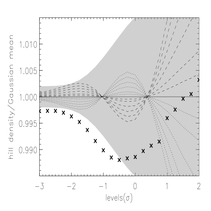
The results of these simulations are shown in the left panel of Figure 1, where we can see the effect for the different values of $f_{\rm NL}$ on the hill density. We applied this procedure to the publicly available WMAP data. We co-added the (foregrounds subtracted) maps from the three WMAP frequency channels Q, U and W following the procedure in [Bennett et al. 2003]. In Figure 2 we show the $\chi^{2}({\tiny f_{\rm NL}})$ for the data around its minimum in the two cases, with and without the off-diagonal elements of the covariance matrix. When using only the diagonal parts of the covariance matrix we estimate $f_{\rm NL}=30$ with a $68\%$ and $95\%$ credible region equal to $-50<f_{\rm NL}<140$ and $-170<f_{\rm NL}<240$, respectively, in good agreement with previously released estimates [Komatsu et al. 2003, Mukherjee & Wang 2004]. We also include proper (frequentist) confidence intervals, which turn out to be $-230<f_{\rm NL}<280$ and $-540<f_{\rm NL}<570$, respectively. The relationship between the two approaches is discussed in subsection 3.4. When including the full covariance matrix, we estimate $f_{\rm NL}=-10$ with a $68\%$ and $95\%$ approximate credible region equal to $-120<f_{\rm NL}<120$ and $-270<f_{\rm NL}<260$ respectively, while the frequentist constraints turn out to be $-140<f_{\rm NL}<120$ and $-280<f_{\rm NL}<300$. We observe that when not including the full covariance matrix, there is a huge difference in error bars between the Bayesian/frequentist approaches. Including the full matrix, this difference is smaller but persists. The much bigger frequentist error bars can be explained as follows: when assuming that the thresholds are uncorrelated, huge deviations from the expected value at many thresholds provide strong evidence against the model to be tested. On the other hand, taking into account the fact that the thresholds are highly correlated, the evidence becomes weaker and the expected model can still be consistent with the observations. Note further that Bayesian error bars tend to be lower than in the frequentist case in the above estimates from the WMAP data; the same phenomenon occurs in simulated maps.
As a final remark, we note that equation (12) can be exploited to implement a goodness-of-fit test for our specification of noise and foreground features. More precisely, we compared the best fit value $\chi(f_{\rm NL}=30)$ obtained for the WMAP data with $\min\chi(f_{\rm NL})$ from 200 Monte Carlo simulations of non-Gaussian CMB maps with $f_{\rm NL}=30$. When using the diagonal covariance matrix, the observed value corresponds to the $28\%$ quantile, thereby suggesting good agreement between WMAP data and our simulated models. When we adopt the full covariance matrix, the observed value is smaller than $92\%$ of the simulations, that is, the local curvature statistics on WMAP data are closer to their expected values than the great majority of simulated maps. Note however that we are performing four similar tests on the data (local curvature, wavelets with and without covariance matrix) and therefore a $92\%$ deviation from simulations is not significant.

Figure 1: On the left, density of hills as a function of the threshold $\nu$, for different values of $f_{\rm NL}$. All values are divided by the Gaussian expectation value. On the right, skewness of wavelet coefficients for different scales $R$. The solid line represents Gaussian simulations, the dotted (dashed) lines represent non-Gaussian simulations for different negative (positive) values of $f_{\rm NL}$; the grey band is the $1\sigma$ confidence level taking into account the noise and beam of the co-added Q+V+W map with an extended Kp0 mask. The values of $|f_{\rm NL}|$ shown are 50, 100, 200, 300, 400 and 500, showing an increasing distance from the Gaussian expectation value. The bold crosses show the results on the data.

Figure 2: The plot shows the $\chi^{2}$ as a function of $f_{\rm NL}$ around its minimum, using the curvature test (left) and the wavelets (right) on the co-added Q+W+V WMAP map. Results including the full covariance matrix are plotted as a dotted line, whereas the solid line corresponds to the diagonal matrix approximation.

3.2 Spherical Wavelets

Wavelets are a very flexible tool used in connection with CMB data for denoising [Sanz et al. 1999], extracting point sources [Cayón et al. 2000, Tenorio et al. 1999], and detecting non-Gaussianity [Cabella et al. 2004, Martínez-González et al. 2002, Barreiro & Hobson 2001, Forni & Aghanim 2001, Starck, Aghanim & Forni 2004]. To test the consistency of our maps of primordial non-Gaussian models with those of [Komatsu et al. 2003] we have repeated the method for estimating $f_{\rm NL}$ described in MW. The basics steps for the test are the following (for more details, see MW):

• we generate a set of primordial non-Gaussian maps with the method described in Section 2 with the WMAP best fit power spectrum and different $f_{\rm NL}$;

• we add noise and convolve with a beam corresponding to the given experiment;

• we apply the Kp0 galactic cut, leaving the point sources unmasked;

• we degrade the maps to the resolution of nside = 256;

• we obtain the wavelet coefficients by convolving each map with the Spherical Mexican Hat Wavelet (SMHW) given by:

  $$\Psi(y,R)=\frac{1}{\sqrt{2\pi}N(R)}\left[1+\left(\frac{y}{2}\right)^{2}\right]^{2}\left[2-\left(\frac{y}{R}\right)^{2}e^{-y^{2}/2R^{2}}\right],$$ (13)

  using the scales $R$ given in MW (14, 25, 50, 75, 100, 150, 200, 250, 300, 400, 500, 600, 750, 900, 1050 arcmin) ;

• we use only the coefficients outside an extended Kp0 mask (for details of the extensions, see [Vielva et al. 2004] and MW) to obtain the skewness as a function of $f_{\rm NL}$. The result is shown in the right panel of Figure 1;

• we finally repeat the last three steps for the data of the given experiment.

• for each simulation as well as for the data, we construct a $\chi^{2}$ as follows

  $$\chi^{2}(f_{\rm NL})=(\mathbf{x}-\langle\mathbf{x}\rangle)^{T}{\mathbf{M}}^{-1}(\mathbf{x}-\langle\mathbf{x}\rangle),$$ (14)

  where the elements of the vector $\mathbf{x}$ are $x_{i}=S(R_{i})$ where $S(R_{i})$ is the skewness of the wavelet coefficients on scale $R_{i}$. The covariance matrix ${\mathbf{M}}$ with elements $M_{ij}=\langle x_{i}x_{j}\rangle$ is evaluated on the basis of 1000 Gaussian simulations. The distribution of the skewness at each scale is close to Gaussian, justifying the above form of the $\chi^{2}$.

• For each simulations and for the data we estimate $f_{\rm NL}$ by minimising this $\chi^{2}$ with respect to the parameter.

• Bayesian error bars are found by constructing the likelihood $L(f_{\rm NL})\propto e^{-\chi^{2}/2}$. Integrating this likelihood with respect to the parameter, we obtain the approximate Bayesian credible regions (see Section 3.4).

• The frequentist error bars are derived by the histogram of the estimates $\hat{f}_{\rm NL}$ from simulations and defining the $1$ and $2\sigma$ levels as the limits within which $68\%$ and $95\%$ of the estimates fall.

Again, the test was performed on the co-added (foreground cleaned) Q+V+W WMAP map. The plot of the $\chi^{2}$ for the data is shown in Figure 2. We estimate the Bayesian credible region, considering only the diagonal part of the covariance matrix (the results presented in MW were obtained using the same approximation), for $f_{\rm NL}$ to be $40\pm 90$ at the 1$\sigma$ level and $40\pm 180$ at the 2$\sigma$ level, in agreement with the values derived in MW (see again the discussion in Section 3.4). Considering the full covariance matrix, we estimate $f_{\rm NL}$ to be $0\pm 120$ at the 1$\sigma$ level and $0\pm 240$ at the 2$\sigma$ level As for the curvature, we have also calculated the frequentist confidence intervals which in the first case turn out to be quite larger, $-100<f_{\rm NL}<170$ and $-230<f_{\rm NL}<320$ respectively, while considering the full covariance matrix we find for the error bars on $f_{\rm NL}$ $-130<f_{\rm NL}<120$ and $-260<f_{\rm NL}<230$. Again the Bayesian credible regions are generally smaller than the frequentist confidence levels, but considering the full covariance matrix, the difference is reduced. Note further that the Bayesian credible regions are slightly underestimated when approximating the covariance matrix to be diagonal.

As before, we also implemented a goodness-of-fit test based on Eq. (14); we found that the values on the WMAP data corresponds to the $32\%$ and $54\%$ quantile obtained from 200 simulations with $f_{\rm NL}=40$ when using the diagonal and full covariance matrices, respectively. Again, this suggests that our specification of noise and foreground masks provides a reasonable approximation to the experimental settings of WMAP.

3.3 The combined test

In this section we apply the combined procedure introduced in [Cabella et al. 2004] to improve the constraints on $f_{\rm NL}$. First of all, we estimated the correlation between the two estimators $\hat{f}_{\rm NL}^{wav}$ and $\hat{f}_{\rm NL}^{cur}$ by 200 Monte Carlo simulations and found

$$\frac{\langle\hat{f_{\rm NL}}^{cur}\hat{f_{\rm NL}}^{wav}\rangle-\langle\hat{f_{\rm NL}}^{cur}\rangle\langle\hat{f_{\rm NL}}^{wav}\rangle}{\sigma^{cur}\sigma^{wav}}\simeq 0.086,$$ (15)

suggesting that the correlation between the estimators is less than $10\%$. Then, we can lower the error bars on $f_{\rm NL}$ by combining the two statistics. More precisely, we use the estimates obtained with the full covariance matrix and we evaluate the frequentist confidence intervals on the following statistic:

$$\hat{f}_{\rm NL}^{comb}=\frac{\hat{f}_{\rm NL}^{wav}+\hat{f}_{\rm NL}^{cur}}{2}.$$ (16)

Using the combined test on the WMAP data, we estimate $f_{\rm NL}=-5$, with the constrains at $1\sigma$ and $2\sigma$ levels of $-90<f_{\rm NL}<80$ and $-180<f_{\rm NL}<170$, respectively.

3.4 A remark on confidence intervals and credible regions on $f_{\rm NL}$

In this subsection we present a brief discussion on the evaluation of (frequentist) confidence intervals and (Bayesian) credible regions on $f_{\rm NL}$. Let us denote by $\widehat{f}_{\rm NL}^{\ast}$ our estimate of the non-linearity parameter obtained by minimising Eqs. (12) and (14): also, let us denote by $L(f_{\rm NL};\widehat{f}_{\rm NL}^{\ast})$ the likelihood function. As well known, an $(1-\alpha)$-level confidence interval for $f_{\rm NL}$ based upon the observation $\widehat{f}_{\rm NL}^{\ast}$ is the set of all values $f_{\rm NL}$ such that

$$\int_{|\widehat{f}_{\rm NL}-f_{\rm NL}|\geq|\widehat{f}_{\rm NL}^{\ast}-f_{\rm NL}|}L(f_{\rm NL};\widehat{f}_{\rm NL})d\widehat{f}_{\rm NL}\geq\alpha.$$

Note that the integral is taken with respect to the estimate $\widehat{f}_{\rm NL}$ that is, we are viewing $L(f_{\rm NL};\widehat{f}_{\rm NL})$ as the probability density of our estimator. In words, we include in the confidence interval all the values $f_{\rm NL}$ such that the probability to get an estimated parameter as $\widehat{f}_{\rm NL}^{\ast}$ or further away is at least as large as $\alpha$. More clearly, a value is included provided it does not entail that observing what we observed is less probable than $\alpha$. Of course, in the special case where the distribution of $\widehat{f}_{\rm NL}$ is Gaussian with mean $f_{\rm NL}$ and variance $\sigma^{2}$ which does not depend on $f_{\rm NL}$ (or, in general, is symmetric under the exchange of $f_{\rm NL}$ and $\widehat{f}_{\rm NL}$), we have

$$\int_{|\widehat{f}_{\rm NL}-f_{\rm NL}|\geq|\widehat{f}_{\rm NL}^{\ast}-f_{\rm NL}|}L(f_{\rm NL};\widehat{f}_{\rm NL})d\widehat{f}_{\rm NL}$$ (17)

$$=\int_{|\widehat{f}_{\rm NL}-f_{\rm NL}|\geq|\widehat{f}_{\rm NL}^{\ast}-f_{\rm NL}|}\frac{1}{\sqrt{2\pi}\sigma}\exp\left\{-\frac{1}{2}(\widehat{f}_{\rm NL}-f_{\rm NL})^{2}\right\}d\widehat{f}_{\rm NL}$$ (18)

$$=\int_{|\widehat{f}_{\rm NL}-f_{\rm NL}|\geq|\widehat{f}_{\rm NL}^{\ast}-f_{\rm NL}|}\frac{1}{\sqrt{2\pi}\sigma}\exp\left\{-\frac{1}{2}(\widehat{f}_{\rm NL}-f_{\rm NL})^{2}\right\}df_{\rm NL}$$ (19)

by the symmetry of the previous expression with respect to $(\widehat{f}_{\rm NL},f_{\rm NL})$. This justifies the common practice to derive confidence intervals by integrating the likelihood. Rigorously speaking, however, this is no longer justified if the integrand is not symmetric with respect to an exchange of $f_{\rm NL}$ with $\widehat{f}_{\rm NL}$ (for instance if $\sigma$ is not constant with respect to $f_{\rm NL}$). One may then try to justify the integration of the likelihood by a Bayesian viewpoint, by assuming a flat prior and viewing $L(f_{\rm NL};\widehat{f}_{\rm NL})$ as a posterior density function. The resulting set, however, should not be labelled as confidence interval (which is a frequentist concept): it is a Bayesian credible region, which will depend in general on the choice of the prior.

It is occasionally stated that this dependence is overcome by the choice of a flat prior. The latter is claimed to be non-informative by definition: indeed, no physicist would consider a priori equally likely that $f_{\rm NL}$ lies in $[-10,10]$ rather than it is in $[317,337]$ (say); thus a flat prior, although unphysical, is usually justified as a panacea to get objective results. This argument is to some extent misleading, though, as it can be shown by standard counterexamples. Take for instance Eq. (1), and assume for brevity’s sake that $f_{\rm NL}>0$ (otherwise duplicate our argument by symmetry). Then Eq. (1) can be rewritten as

$$T=\phi_{\rm G}({\bf x})+(g_{\rm NL}\phi_{\rm G}({\bf x}))^{2}\;,$$ (20)

that is $f_{\rm NL}=g_{\rm NL}^{2}$. Of course, from the physical point of view there is no reason to prefer the alternative specification in Eq. (1) to (20) . Now let us assume we impose a “non-informative” (flat) prior on $g_{\rm NL}:$, the posterior probability becomes

$$\frac{1}{\sqrt{2\pi}\sigma}\exp\left\{-\frac{1}{2}(\widehat{f}_{\rm NL}-g_{\rm NL}^{2})^{2}\right\}dg_{\rm NL}=\frac{1}{\sqrt{2\pi}\sigma}\exp\left\{-\frac{1}{2}(\widehat{f}_{\rm NL}-f_{\rm NL})^{2}\right\}\frac{df_{\rm NL}}{2\sqrt{f_{\rm NL}}}$$

and the credible sets are thus obviously affected, although we are working with exactly the same model as before and we are claiming to have used no a priori information. In short, flat priors are simply shifting the choice from the form of the prior probability to the form of the statistical parametrisation; the latter, moreover, is not due to physical considerations, but simply to computational convenience.

With this in mind, we will now use $\widehat{f}_{\rm NL}$ estimated from 200 simulations (with the experimental settings used above) to investigate whether the distribution of $\widehat{f}_{\rm NL}$ as a function of the model $f_{\rm NL}$ is symmetric with respect to an exchange of $f_{\rm NL}$ and $\widehat{f}_{\rm NL}$. In Figures (3), (4) we show a contour plot of this function for the curvature and wavelet test, respectively. When not considering the full covariance matrix, this function is markedly skewed for the wavelet test, but even more so for the curvature test (see fig. 3) . This may explain the big difference between the confidence intervals and Bayesian credible regions for the wavelets and the even bigger difference for the curvature test when correlations are neglected. On the other hand, when correlations are properly taken into account, the model fit is better and the function becomes considerably more symmetric (see fig. 4). This is also reflected in the fact that the difference between Bayesian and frequentist error bars is markedly reduced in this case .

Figure 3: The distribution of estimates $\widehat{f}_{NL}$ as a function of the model parameter $f_{NL}$. The isocontours of the distribution is plotted in terms of percentages of the number of maps used in the simulations. The distribution is clearly skewed with respect to the diagonal shown for clarity. The estimates of $f_{\textrm{NL}}$ were obtained using the curvature method (left plot) and wavelets (right plot).

Figure 4: As Fig. 3 but by using the full correlation matrix. The skewness of the distribution is clearly reduced with respect to the diagonal case (see Fig. 3). The estimates of $f_{\textrm{NL}}$ were obtained using the curvature method (left plot) and wavelets (right plot).

4 Conclusions

In this paper we have used simulated CMB maps of primordial non-Gaussian models, generated with the algorithm described in [Liguori, Matarrese & Moscardini 2003] to estimate the non-linear coupling parameter $f_{\rm NL}$ from the WMAP data. As all other estimates of $f_{\rm NL}$ in the literature have been based on non-Gaussian CMB maps generated by a different approach [Komatsu et al. 2003], one of the aims of this paper was to check whether a different way of generating CMB maps with the same kind of primordial non-Gaussianity gives a consistent estimate of $f_{\rm NL}$. In order to perform a direct test of consistency, we applied the estimator of $f_{\rm NL}$ using SMHW presented in [Mukherjee & Wang 2004] on the WMAP data. When neglecting the scale-scale correlations, we find that our estimate of $f_{\rm NL}$ is in full agreement with theirs and thus that the two ways of generating primordial non-Gaussian maps give fully consistent results. We have also presented a new method to estimate $f_{\rm NL}$ based on the local curvature of the CMB fluctuation field. Our estimate of $f_{\rm NL}$ with this method on the WMAP data is consistent with estimates of $f_{\rm NL}$ using other approaches.

Moreover, we point out the importance of including the full covariance matrix in the $\chi^{2}$ when estimating $f_{\rm NL}$ with these two methods. We also discuss the difference between frequentist confidence intervals and Bayesian credible regions on the estimate of $f_{\rm NL}$. We show that the difference between these two methods for finding error bars can be huge when not including the full covariance matrix, particularly for the curvature estimator where correlations between thresholds are important. For the WMAP data, the Bayesian credible region expands whereas the frequentist confidence intervals shrink when taking into account correlations in the covariance matrix. We find further that the Bayesian credible regions are in general smaller than the frequentist confidence intervals. We conclude that care must be taken when approximating the confidence intervals on $f_{\rm NL}$ using the integral of the likelihood with respect to the parameter.

Including the full covariance matrix, we find with the curvature method $f_{\rm NL}=-10^{+310}_{-270}$ at the $2\sigma$ level using frequentist confidence intervals, and $f_{\rm NL}=-10^{+270}_{-260}$ using Bayesian credible regions. Similarly for the wavelet method, $f_{\rm NL}=0^{+230}_{-260}$ with frequentist confidence intervals and $f_{\rm NL}=0^{+240}_{-240}$. Finally, we show that the two methods provide approximately uncorrelated estimates of $f_{\rm NL}$; this observation naturally suggests an improved estimator which combines the two methods. With this combined test, we find $f_{NL}=-5\pm 85$ and $f_{NL}=-5\pm 175$ at the $1\sigma$ and $2\sigma$ level respectively.

References

- [Acquaviva et al. 2003] Acquaviva V., Bartolo N., Matarrese S., Riotto A., 2003, Nucl. Phys. B667, 119
- [Alishahiha, Silverstein & Tong 2004] Alishahiha M., Silverstein E., Tong D., 2004, preprint (hep-th/0404084)
- [Arkani-Hamed et al. 2004] Arkani-Hamed N., Creminelli P., Mukohyama S., Zaldarriaga M., 2004, JCAP, 04, 001
- [Barreiro & Hobson 2001] Barreiro R.B., Hobson M.P., 2001, MNRAS, 327, 813
- [Bartolo, Matarrese & Riotto 2002] Bartolo N., Matarrese S., Riotto A., 2002, Phys. Rev., D65, 103505
- [Bartolo, Matarrese & Riotto 2004a] Bartolo N., Matarrese S., Riotto A., 2004a, JCAP, 0401, 003
- [Bartolo, Matarrese & Riotto 2004b] Bartolo N., Matarrese S., Riotto A., 2004b, JHEP, 0404, 006
- [Bartolo, Matarrese & Riotto 2004c] Bartolo N., Matarrese S., Riotto A., 2004c, Phys. Rev., D69, 043503
- [Bennett et al. 2003] Bennett C.L. et al., 2003, ApJS, 148, 1
- [Bernardeau & Uzan 2002] Bernardeau F., Uzan J.-P., 2002, Phys. Rev., D66, 103506
- [Bernardeau & Uzan 2003] Bernardeau F., Uzan J.-P., 2003, Phys. Rev., D67, 121301
- [Cabella 2004] Cabella P., Ph.D. Thesis, 2004, University of ’Tor Vergata’, Rome
- [Cabella et al. 2004] Cabella P., Hansen F., Marinucci D., Pagano D., Vittorio N., 2004, Phys. Rev., D69, 063007
- [Cayón et al. 2003] Cayón L., Martínez-González E., Argeso F., Banday A.J., Górski K.M., 2003, MNRAS, 339, 1189
- [Cayón et al. 2000] Cayón L., Sanz J.L., Barreiro R.B., Martínez-González E., Vielva P., Toffolatti L., Silk J., Diego J.M., Argeso F., 2000, MNRAS, 315, 757
- [De Troia et al. 2003] De Troia G. et al., 2003, MNRAS, 343, 284
- [Dorè et al. 2003] Dorè O., Colombi S., Bouchet F.R., 2003, MNRAS, 344, 905
- [Dvali, Gruzinov & Zaldarriaga 2004] Dvali G., Gruzinov A., Zaldarriaga M., 2004, Phys. Rev., D69, 083505
- [Enqvist & Sloth 2002] Enqvist K., Sloth M.S., 2002, Nucl. Phys., B626, 395
- [Enqvist & Vaihkonen 2004] Enqvist K., Vaihkonen A., 2004, JCAP, 0409, 006
- [Falk, Rangarajan & Srednicki 1993] Falk T., Rangarajan R., Srednicki M., 1993, ApJ, 403, L1
- [Forni & Aghanim 2001] Forni O., Aghanim N., 2001, A&AS, 137, 553
- [Gangui et al. 1994] Gangui A., Lucchin F., Matarrese S., Mollerach S., 1994, ApJ 430, 447
- [Gaztañaga & Wagg 2003] Gaztañaga E., Wagg J., 2003, Phys. Rev., D68, 021302
- [Górski et al. 1998] Górski K.M., Hivon E., Wandelt B.D., 1998, Analysis Issues for Large CMB Data Sets, eds. A.J. Banday, R.K. Sheth and L. Da Costa, ESO, Printpartners Ipskamp, NL, pp.37-42
- [Hansen et al. 2004] Hansen F.K., Cabella P., Marinucci D., Vittorio N., 2004, ApJ, 607, L67
- [Hansen, Marinucci & Vittorio 2003] Hansen F.K., Marinucci D., Vittorio N., 2003, Phys. Rev., D67, 123004
- [Hansen et al. 2002] Hansen F.K., Marinucci D., Natoli P., Vittorio N., 2002, Phys. Rev., D66, 063006
- [Kofman 2003] Kofman L., 2003, preprint (astro-ph/0303614)
- [Komatsu & Spergel 2001] Komatsu E., Spergel D.N., 2001, Phys. Rev., D63, 063002
- [Komatsu, Spergel & Wandelt 2003] Komatsu E., Spergel D.N., Wandelt B.D., 2003, preprint (astro-ph/0305189)
- [Komatsu et al. 2002] Komatsu E., Wandelt B.D., Spergel D.N., Banday A.J., Górski K.M., 2002, ApJ, 566, 19
- [Komatsu et al. 2003] Komatsu E. et al. 2003, ApJS, 148, 119
- [Liguori, Matarrese & Moscardini 2003] Liguori M., Matarrese S., Moscardini L., 2003, ApJ, 597, 57 (LMM)
- [Liguori, Matarrese & Riotto 2004] Liguori M., Matarrese S., Riotto A., 2004, in preparation
- [Lesgourgues, Polarski & Starobinsky 1997] Lesgourgues J., Polarski D., Starobinsky A.A., 1997, Nucl. Phys., B497, 479
- [Lyth, Ungarelli & Wands 2003] Lyth D., Ungarelli C., Wands D., 2003, Phys. Rev., D67, 023503
- [Lyth & Wands 2002] Lyth D., Wands D., 2002, Phys. Lett., B524,5
- [Maldacena 2002] Maldacena J., 2002, JHEP, 0305, 013
- [Martínez-González et al. 2002] Martínez-González E., Gallegos J.E., Argeso F., Cayón L., Sanz J.L., 2002, MNRAS, 336, 22
- [Matarrese & Riotto 2003] Matarrese S., Riotto A., 2003, JCAP, 0308, 007
- [Mollerach 1990] Mollerach S., 1990, Phys. Rev., D42, 313
- [Moroi & Takahashi 2001] Moroi T., Takahashi T., 2001, Phys. Lett., B522, 215
- [Moroi & Takahashi 2002] Moroi T., Takahashi T., 2002, Phys. Rev., D66, 063501
- [Mukherjee & Wang 2004] Mukherjee P., Wang Y., 2004, ApJ, 613, 51
- [Salopek & Bond 1990] Salopek D.S., Bond J.R., 1990, Phys. Rev., D42, 3936
- [Salopek & Bond 1991] Salopek D.S., Bond J.R., 1991, Phys. Rev., D43, 1005
- [Santos et al. 2003] Santos M.G. et al., 2003, MNRAS, 341, 623
- [Sanz et al. 1999] Sanz J.L., Argeso F., Cayón L., Martínez-González E., Barreiro, R.B., Toffolatti L., 1999, MNRAS, 309, 672
- [Schmalzing & Górski 1998] Schmalzing J., Górski K.M., 1998, MNRAS, 297, 355
- [Seljak & Zaldarriaga 1996] Seljak U., Zaldarriaga M., 1996, ApJ, 469, 437
- [Starck, Aghanim & Forni 2004] Starck J.-L., Aghanim N., Forni O., 2004, A&A, 416, 9
- [Tenorio et al. 1999] Tenorio L., Jaffe A.H., Hanany S., Lineweaver C.H., 1999, MNRAS, 310, 823
- [Varshalovich et al. 1988] Varshalovich D.A., Moskalev A.N., Khersonskii V.K., 1988, ’Quantum theory of angular momentum’ (World Scientific Publishing)
- [Verde et al. 2000] Verde L., Wang L., Heavens A.F., Kamionkowski M., 2000, MNRAS, 313, 141
- [Vielva et al. 2004] Vielva P., Martìnez-Gonzàlez E., Barreiro R.B., Sanz J.L., Cayon L., ApJ, 609, 22
- [Wands et al. 2002] Wands D., Bartolo N., Matarrese S., Riotto A., 2002, Phys. Rev., D66, 043520
- [Wang & Kamionkowski 2000] Wang L., Kamionkowski M., 2000, Phys. Rev., D61, 063504
- [Zaldarriaga 2004] Zaldarriaga M., 2004, Phys. Rev., D69, 043508