MEASURING THE RADIATIVE HISTORIES OF HIGH-REDSHIFT QSOs WITH THE TRANSVERSE PROXIMITY EFFECT

Abstract

Since the photons that stream from QSOs alter the ionization state of the gas they traverse, any changes to a QSO’s luminosity will produce outward-propagating ionization gradients in the surrounding intergalactic gas. This paper shows that at redshift $z\sim 3$ the gradients will alter the gas’s Lyman-$\alpha$ absorption opacity enough to produce a detectable signature in the spectra of faint background galaxies. By obtaining noisy (S:N$\sim 4$) low-resolution ($\sim 7$Å) spectra of a several dozen background galaxies in a $R\sim 20^{\prime}$ field surrounding an isotropically radiating 18th magnitude QSO at $z=3$, it should be possible to detect any order-of-magnitude changes to the QSO’s luminosity over the previous 50–100 Myr and to measure the time $t_{Q}$ since the onset of the QSO’s current luminous outburst with an accuracy of $\sim 5$ Myr for $t_{Q}\lower 2.15277pt\hbox{$\;\buildrel<\over{\sim}\;$}50$ Myr. Smaller fields-of-view are acceptable for shorter QSO lifetimes. The major uncertainty, aside from cosmic variance, will be the shape and orientation of the QSO’s ionization cone. This can be determined from the data if the number of background sources is increased by a factor of a few. The method will then provide a direct test of unification models for AGN.

1. INTRODUCTION

The $10^{8}$-$M_{\odot}$ black holes that lie at the heart of nearby bulge galaxies are believed to have accreted much of their mass in their youths when they shone briefly and brightly as QSOs (e.g., Yu & Tremaine 2002). A great deal could be learned about the physical processes that produce super-massive black holes if we could observe how their brightnesses varied during this time. For example, a black hole that radiates at a fraction $l\equiv L/L_{E}$ of its Eddington luminosity and accretes mass with radiative efficiency $\epsilon\equiv L/\dot{M}c^{2}$ requires $t_{S}\sim M_{\rm BH}/\dot{M}_{\rm BH}\sim 4\times 10^{7}l(\epsilon/0.1)$ yrs to change its mass significantly. Showing that QSO outbursts have a much shorter duration would confirm the popular belief (e.g., Haehnelt & Kauffmann 2000; Cavaliere & Vittorini 2000; Wyithe & Loeb 2002; Di Matteo et al. 2003) that super-massive black holes build up their masses through numerous accretion episodes. Various theoretical attempts to explain the observed correlation between a black hole’s mass and its bulge’s velocity dispersion (e.g., Silk & Rees 1998; Adams, Graff, & Richstone 2001; Burkert & Silk 2001; Miralda-Escudé & Kollmeier 2004) each postulate different physical mechanisms that quench the QSO’s luminosity when it reaches a certain level. To the extent that these mechanisms operate on different time scales, measuring the duration of QSO outbursts should help us distinguish between them.

The challenge is to figure out from a few short nights or decades of observations how a QSO’s brightness changed over the preceding few million years. Investigators have resorted to a number of indirect schemes. By making assumptions about the link between QSOs and either local black holes or massive potential wells at the redshift of observation, several authors have deduced that individual QSOs are unlikely to have shone for fewer than 1Myr or more than 100Myr (e.g., Haehnelt, Natarajan, & Rees 1998; Richstone et al. 1998; Martini & Weinberg 2001; Hosokawa 2002). Unfortunately the uncertain underlying assumptions do not seem to allow a much more precise limit on the typical QSO lifetime. In any case statistical arguments like these will never be able to tell whether a QSO’s total radiative lifetime of (say) $10^{7}$ yr occurred in one contiguous chunk or was instead split among numerous shorter bursts, though this distinction could be crucial in developing a physical picture of black-hole formation.

This paper describes a method that is somewhat less indirect and that can provide a rough indication of how any given QSO’s luminosity varied over the $50$–100 Myr preceding the time of observation. The simple idea behind the method is illustrated in Figure 1. Although we cannot detect the photons a QSO emitted in the past, we can detect their effect on its surroundings. As hydrogen-ionizing photons from a QSO propagate outwards, they destroy neutral hydrogen in the intergalactic medium and reduce the number of Lyman-$\alpha$ absorption lines in the spectra of background objects. The change in the Lyman-$\alpha$ opacity at radius $r$ should therefore provide some indication of the QSO’s luminosity at the earlier time $t\sim r/c$. The rest of the paper works out this simple idea in more detail. § 2 presents a brief review of the relevant intergalactic physics and justifies two assumptions that will be needed later. §§ 3 and 4 work out the effect of changes in the QSO’s luminosity on background galaxies’ spectra. The next two sections discuss the significance with which the effect can be detected: § 5 treats the uncertainties from a theoretical point-of-view and concludes that cosmic variance will be the primary problem, while § 6 discusses the spectroscopic exposure times that will be necessary on a 10m telescope and argues that neither continuum removal nor interstellar absorption lines will be a major obstacle. The results from the preceding sections are brought together in one place in § 7, which presents a sample analysis of a simulated QSO with a known radiative history. Some readers may wish to skip directly to this section. § 8 discusses the time resolution that can be achieved with this technique. My main conclusions are reviewed and criticized in § 9.

I should state at the outset that this is not the only method for constraining the radiative histories of individual QSOs. Readers may judge for themselves the relative merits of the alternatives that are listed (e.g.) in the excellent review by Martini (2003). Nor is the idea behind the method new. Jakobsen et al. (2003) have used it, for example, to estimate an age of $t>10^{7}$yr for the QSO Q03022-0023 from the lack of absorption lines in the spectrum of a neighboring QSO. Schirber, Miralda-Escudé, & McDonald (2004) and Croft (2004) applied a similar analysis to a larger sample of QSO pairs and inferred significantly shorter lifetimes. What is new, as far as I know, is the assumption that the background sources will be numerous faint galaxies rather than a single bright QSO. This complicates the analysis in a number of ways but yields a considerably more detailed view of the foreground QSO’s radiative history.

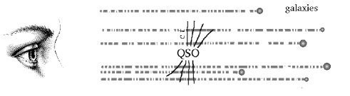
Figure 1.— Schematic view of the underlying concept. QSOs emit H-ionizing radiation that will destroy some of the HI in the intergalactic medium out to a maximum radius $ct_{Q}$, where $t_{Q}$ is the time since the onset of QSO activity. HI in the intergalactic medium produces absorption lines in the spectra of background objects. The absorption is represented by a broken line between the objects and the observer; breaks in the line mark positions with significant HI absorption. By obtaining spectra of numerous galaxies that lie behind a high-redshift QSO, one can (a) map the spatial distribution of intergalactic HI around the QSO, (b) use the shape of the region with lowered HI absorption to estimate the rough geometry of the intergalactic volume that has been hit by the QSO’s radiation, and (c) deduce the QSO’s lifetime and the level of anisotropy in its emission.

2. PRELIMINARIES

The low observed level of Lyman-$\alpha$ absorption from intergalactic gas at $z\sim 3$ implies that the gas must be almost completely ionized, with perhaps only one neutral H atom per million (Gunn & Peterson 1965). As a result the typical hydrogen ionizing photon will travel far before it is absorbed, $\sim 50$ proper Mpc ($\Omega_{M}=0.3$, $\Omega_{\Lambda}=0.7$, $h=0.65$; Madau, Haardt, & Rees 1999), and one can safely assume that intergalactic gas is optically thin on length scales significantly smaller. Radiation from distant sources will permeate this optically thin gas at a roughly uniform level $J_{\rm bg}$, ionizing residual hydrogen atoms at a rate $\Gamma^{\rm bg}_{\gamma}n_{HI}$ where $n_{HI}$ is the neutral hydrogen density and

$$\Gamma^{\rm bg}_{\gamma}\equiv\int_{13.6{\rm eV}}^{\infty}\!\!\!\!\!\!\!\!\!\!\!dE\,4\pi J_{\rm bg}(E)\sigma_{i}(E)/E$$ (1)

is an integral over energy of the photon number density times the hydrogen photoionization cross-section $\sigma_{i}$. For plausible intensities of the background radiation field, e.g.,

$$J_{\rm bg}(\nu)\sim 10^{-21.3}(h\nu/13.6{\rm eV})^{-1.8}{\rm erg}\,{\rm s}^{-1}{\rm cm}^{-2}{\rm sterad}^{-1}{\rm Hz}^{-1},$$ (2)

and for densities near the cosmic mean, photon absorption will be the dominant ionization pathway for hydrogen, and the neutral fraction $\eta$ of intergalactic gas will adjust itself until the photoionization rate is equal to the recombination rate $\alpha_{\mathit{H}II}n_{\mathit{H}II}n_{e}$:

$$\eta\equiv\frac{n_{\mathit{H}I}}{n_{\mathit{H}I}+n_{\mathit{H}II}}\simeq\frac{\alpha_{\mathit{H}II}n_{e}}{\Gamma_{\gamma}}.$$ (3)

The recombination coefficient has a temperature dependence that is well fit by the expression $\alpha_{\mathit{H}II}\simeq 2.11\times 10^{-14}T_{6}^{-0.7}(1+T_{6}^{0.7})^{-1}$ cm³ s^-1 where $T_{6}$ is the temperature in units of $10^{6}$ K (Cen 1992).

Now consider what happens to intergalactic gas when it is hit by a blast of ionizing radiation from a nearby QSO. The photoionization rate increases by an amount $\Gamma^{Q}_{\gamma}$, given by equation 2 with the QSO’s radiation field $J_{Q}$ replacing $J_{\rm bg}$, and the neutral fraction $\eta$ falls to its new equilibrium value $\eta_{\rm new}=\eta_{\rm old}\Gamma^{\rm bg}_{\gamma}/(\Gamma^{\rm bg}_{\gamma}+\Gamma^{Q}_{\gamma})$ on the time scale $|n_{\mathit{H}I}/\dot{n}_{\mathit{H}I}|\sim 1/\Gamma^{Q}_{\gamma}$, or $\sim 10^{4}$ yr if $J_{Q}$ is equal to the background intensity $J_{\rm bg}$. After the blast subsides, recombination will raise the neutral density back to its previous level on the same time-scale.

In contrast to the potentially large swings in the gas’s neutral fraction, any changes to its temperature should be imperceptibly slight. Although the gas will warm as photo-electrons collide with other particles and distribute their kinetic energy, the change in its total thermal energy will be negligible: photo-electrons are necessarily as rare as neutral atoms ($\sim 1$ppm) and their typical kinetic energy at ejection

$$\epsilon_{HI} = (\Gamma^{Q}_{\gamma})^{-1}\int_{E_{\rm th}}^{\infty}\!\!\!\!dE\,4\pi J_{Q}(E)\sigma_{i}(E)(E-E_{\rm th})/E$$

$$= E_{\rm th}/(2+s)\simeq 3.6{\rm eV}\quad{\rm for}\quad J_{Q}(E)\propto E^{-s},$$

$$\quad\quad s=1.8,\,\,\sigma_{i}(E)\propto E^{-3},\,\,E_{\rm th}=13.6{\rm eV}$$

is not very different from the energy per particle in the $\sim 20000$K undisturbed gas. The gas received its energy of about an eV per particle when it was almost completely ionized at earlier times, and its temperature will hardly be affected by giving a few eV to the particle per million that remained neutral. This shows that the temperature of the gas will not rise appreciably while its ionization balance adjusts to the increased ionizing background. Afterwards the gas will be heated by photoionizations at the same rate as before—the increase in photoionization rate per HI atom will be exactly compensated by a decrease in the density of HI atoms—and so the equilibrium temperature will be the same in parts of the IGM that are and are not illuminated by the QSO’s radiation.

Taken together, the results reviewed in this section justify two assumptions that I will adopt for the remainder of the paper. (a) If a QSO’s luminosity towards solid angle $\Omega$ at time $t$ is $L(\Omega,t)$, then the intensity of the QSO’s radiation field at position ${\mathbf{r}}$, $\Omega$ at time $t+|{\mathbf{r}}|/c$ will be proportional to $L(\Omega,t)/r^{2}$. In other words, intergalactic gas at larger distances will not be significantly shielded from the QSO’s radiation by intergalactic gas at smaller distances. (b) The intergalactic temperature will not be affected by changes in the intensity of ionizing radiation. This implies first that a blast of radiation from a QSO will alter the ionization balance of intergalactic gas but not its spatial or velocity structure, and second that any changes in neutral fraction will be precisely proportional to the change in the ionizing radiation density (equation 3 with constant $\alpha_{HII}$) averaged over the last $\sim 10^{4}$ yr.

3. MEAN TRANSMISSIVITY VERSUS $J_{\nu}$

We will be able to measure changes in a QSO’s ionizing history with this method only if we can detect spatial changes in the surrounding density of neutral hydrogen. Intergalactic HI density is normally measured by fitting Voigt profiles to the numerous Lyman-$\alpha$ absorption lines in the spectra of background QSOs. This approach is not feasible when the background sources are faint galaxies, since individual Lyman-$\alpha$ forest absorption lines are hopelessly blended and confused in their noisy low-resolution spectra. Instead we can only hope to measure $\bar{f}\equiv\langle e^{-\tau_{{\rm Ly}\alpha}}\rangle$, the mean transmissivity along a spectral segment whose length of a few Å is many times larger than the typical absorption-line spacing but comparable to the instrumental resolution. Although a reliance on $\bar{f}$ is forced on us, $\bar{f}$ has two advantages over $n_{\rm HI}$ as a probe of the ionizing background radiation. First, it receives significant contributions from the parts of the IGM with middling HI optical depths $\tau_{{\rm Ly}\alpha}\sim 1$ whose response to changes in the ionizing radiation are easiest to measure. In contrast $\bar{n}_{\rm HI}$ is dominated by systems with large optical depths, and since $e^{-\tau}\simeq e^{-2\tau}\simeq 0$ for large $\tau$, big changes in the column densities of optically thick systems can be hard to detect. Second, the value of $\bar{n}_{\rm HI}$ along any particular line-of-sight is strongly affected by whether the line happens to pierce an especially dense system. This adds to $\bar{n}_{\rm HI}$ large random fluctuations that may obscure underlying changes in the radiation field. $\bar{f}$ weights more evenly across systems of different column densities and is consequently less affected by chance fluctuations in the density of matter, a point that we will elaborate upon in § 5 below.

Let us work out, then, how $\bar{f}$ responds to changes in the ionizing background. As argued in § 2, $\tau$ at fixed total hydrogen density is inversely proportional to the ionizing radiation intensity $J$, and so if the radiation intensity changes from $J$ to $bJ$, with $b$ an arbitrary constant, the new mean transmissivity will be

$$\bar{f}=\int_{0}^{\infty}d\tau\,P(\tau)e^{-\tau/b}$$ (5)

where $P(\tau)$ is the Lyman-$\alpha$ optical-depth distribution that existed before the change.

To estimate $P(\tau)$, I converted published Lyman-$\alpha$ Voigt profile lists for 5 QSOs near $z=3$ into lists of the observed Lyman-$\alpha$ optical depth $\tau$ vs. comoving distance, applied a QSO-dependent scaling to every $\tau$ to make each QSO’s Lyman-$\alpha$ forest have the same mean transmissivity $\bar{f}=0.67$ appropriate to $z=3.00$ (McDonald et al. 2001), and finally constructed a histogram of the resulting $\tau$ values.

The top panel of figure 2 shows the dependence of the mean transmissivity on the radiation intensity, calculated numerically from equation 5 using a spline fit to this histogram as an approximation to $P(\tau)$. Also shown is $\Delta\bar{f}\equiv(d\bar{f}/d\,{\rm ln}J_{Q})$, with $J_{Q}\equiv J_{\nu}-J_{\rm bg}$ the QSO’s contribution to the radiation field. This provides some indication of how strongly $\bar{f}$ responds to large changes in $J_{Q}$. The bottom middle panel presents the $J_{\nu}$–$\bar{f}$ relationship in a slightly different way, as the mean transmissivity as a function of distance $r$ from an isotropically radiating $z=3.0$ QSO with AB magnitude $m_{912}=18$ or $m_{912}=20$ at rest-frame 912Å that has been radiating forever at a constant rate. This panel assumes that the background radiation field $J_{\rm bg}$ (equation 2) would have been spatially uniform in the absence of the QSO, which implies that the actual radiation field is

$$J(r)=\Bigl{[}1+\Bigl{(}\frac{r_{\rm eq}}{r}\Bigr{)}^{2}\Bigr{]}J_{\rm bg}$$ (6)

where

$$r_{\rm eq}\equiv d_{L}(z)\Bigl{[}\frac{f_{\nu}/J_{\rm bg}}{4\pi(1+z)}\Bigr{]}^{1/2},$$ (7)

$f_{\nu}\equiv 10^{-0.4(m_{912}+48.60)}$ is the flux from the QSO received on earth at wavelength $(1+z)\times$912Å and $d_{L}(z)$ is the QSO’s luminosity distance.

Figure 2.— Top panel: the solid line shows dependence of intergalactic Lyman-$\alpha$ transmissivity $\bar{f}\equiv\langle e^{-\tau_{{\rm Ly}\alpha}}\rangle$ at $z=3$ on the intensity $J_{\nu}$ of the ionizing radiation field. The transmissivity $\bar{f}\simeq 0.67$ is appropriate to the actual background ionizing-radiation field $J_{\rm bg}$. Increases in the radiation intensity destroy neutral hydrogen and increase the transmissivity. The curve shown was calculated with equation 5 from Voigt-profile fits to the Lyman-$\alpha$ forest at $z\sim 3$ (see text). The dashed line shows $\Delta\bar{f}\equiv(d\bar{f}/dJ_{\nu})(J_{\nu}-J_{\rm bg})$, which is roughly the change in $\bar{f}$ that would result if the perturbation to the radiation field (i.e., the difference between $J_{\nu}$ and $J_{\rm bg}$) were doubled. Bottom panel: the expected intergalactic transmissivity as a function of distance from a constantly shining QSO with apparent AB magnitude $m_{912}=18$ (solid line) or $m_{912}=20$ (dotted line) at $z=3$. The QSO’s radiation adds to the background radiation $J_{\rm bg}$, which we are taking to be $J_{\rm bg}=5\times 10^{-22}$ erg s^-1 cm^-2 Hz^-1 sr^-1 at $912$Å, and increases the transmissivity in its vicinity.

The top panel implies (for example) that if the mean transmissivity in a given region can be estimated with an uncertainty of $\sigma_{f}\sim 0.04$, then a significant change to the QSO’s luminosity ($\Delta{\rm ln}J_{Q}\sim 1$) will be marginally detectable if the region’s distance to the QSO implies an expected mean transmissivity $0.72\lower 2.15277pt\hbox{$\;\buildrel<\over{\sim}\;$}\bar{f}\lower 2.15277pt\hbox{$\;\buildrel<\over{\sim}\;$}0.93$. The bottom panel shows that the required distance is $12\lower 2.15277pt\hbox{$\;\buildrel<\over{\sim}\;$}r\lower 2.15277pt\hbox{$\;\buildrel<\over{\sim}\;$}2$ proper Mpc for a QSO with $m_{912}=18$. Adopting the crude approximation $t_{\rm delay}\sim-2r/c$ leads to the preliminary guess that the method should provide reasonable constraints on the QSO’s luminosity for time delays of $-10\lower 2.15277pt\hbox{$\;\buildrel>\over{\sim}\;$}t\lower 2.15277pt\hbox{$\;\buildrel>\over{\sim}\;$}-80$ Myr. A more careful treatment is deferred until § 7.

4. TIME-DELAY SURFACE

The actual situation is slightly more complicated than Figure 1 suggests, since light from the background sources does not pass the QSO instantaneously. Instead it encounters material that lies behind the QSO before it encounters material that lies in front, and as a result the observed intergalactic absorption from material behind the QSO will be sensitive to the QSO’s luminosity at an earlier time. If we define $t=0$ as the time when the QSO emitted the light that is just now reaching earth, and if we place the QSO at the origin of a polar coordinate system where R measures proper displacements along the plane of the sky and z measures proper displacements in the redshift direction, then the light from a background galaxy passes through the intergalactic gas that lies a proper distance $z$ behind the QSO at the time $t=-z/c$, and the ionization balance of the gas at this time is sensitive to the QSO’s luminosity at the earlier time

$$t_{I}(R,z)\equiv\bigl{[}-z-(R^{2}+z^{2})^{1/2}\bigr{]}/c.$$ (8)

Figure 3 shows the parabolic contours of this function in astronomically useful units. The figure implies, for example, that the ionization balance of the intergalactic gas that lies 5 Mpc behind the QSO and 2 Mpc to the left will reflect the QSO’s luminosity at time $t=-34$ Myr, while the material that lies directly in front of the QSO will have an ionization balance that reflects the QSO’s luminosity at $t=0$ (i.e., its observed luminosity).

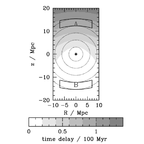
Figure 3.— The time-delay surface. A QSO at the origin emits hydrogen-ionizing radiation into the surrounding intergalactic medium. Concentric circles show the distance that has been traveled traveled by the photons emitted by the QSO at the earlier times $t=-10$, -20, -30, -40, -50 Myr. Photons from background sources at $z\to\infty$ traverse this region from top to bottom as they travel to earth at $z\to-\infty$. At each point along the way they pass photons that were emitted by the QSO at a different time in its past. The shaded contours show the emission time of the QSO photons that were illuminating a given intergalactic region when the observed photons from a background source passed by. The strength of the Lyman-$\alpha$ absorption lines from this region in the spectrum of the background source will depend on the QSO’s luminosity at the indicated time. Averaging together the absorption lines from large regions with the same time delay (e.g., the region marked $A$) can provide a constraint on the QSO’s luminosity at that time. Comparing many such regions allows one to chart historical fluctuations in the QSO’s luminosity. A particularly promising strategy is to estimate the luminosity at the time corresponding to region $A$ ($\sim-90$ Myr) by comparing the absorption lines in $A$ to the absorption lines in a similar region ($B$) on the opposite side of the QSO that is illuminated by QSO photons emitted at $t\sim 0$. Most systematics will cancel out in this binary comparison. See text.

Now the field of view of a large optical imagers is around $40^{\prime}$, or $\sim 19.9h_{65}^{-1}$ proper Mpc at $z=3$ ($\Omega_{M}=0.3$, $\Omega_{\Lambda}=0.7$), and the largest optical multi-object spectrograph (Dressler, Sutin, & Bigelow 2003) on an 8m-class telescope is not much smaller. This makes it relatively easy to obtain spectra of high-redshift galaxies throughout an $r\sim 20^{\prime}$ region centered on a QSO at $z=3$, probing the ionization balance of the IGM in the region of this plot with $-10<R<10$ Mpc. Because more than 1000 background galaxies with redshift $z\lower 2.15277pt\hbox{$\;\buildrel>\over{\sim}\;$}3.0$ and magnitude ${\cal R}\leq 25.5$ will be found in a field of this size with the “UV drop-out” technique (e.g., Steidel et al. 2003), the Lyman-$\alpha$ absorption lines in these galaxies’ spectra can in principle provide an enormously detailed view of the IGM’s ionization balance near the QSO.

Assume, then, that we have measured the intergalactic Lyman-$\alpha$ transmissivity $f\equiv\exp(-\tau_{{\rm Ly}\alpha})$ throughout the region of the figure with $-10<R<10$ Mpc. A number of ways to estimate the evolution of the QSO’s ionizing luminosity suggest themselves immediately. One is to divide the region behind the QSO (i.e., the region with $z>0$ in figure 3) into a number of bins whose edges align with contours of the time delay surface, then see how the mean transmissivity $\bar{f}_{\rm obs}$ in each compares to $\bar{f}_{\rm exp}$, the expected transmissivity if $L(t)$ were constant. Region $A$ in figure 3 is one such bin. The problem is estimating $\bar{f}_{\rm exp}$. This suggests a slight variation: compare $\bar{f}_{\rm obs}$ in each bin to $\bar{f}_{\rm con}$, the mean transmissivity in a bin of the same shape located on the opposite side of the QSO. See (e.g.) regions $A$ and $B$ in the figure. Since $A$ is illuminated by photons emitted at $t\sim-80$ Myr and $B$ is illuminated by photons emitted at $-10{\rm Myr}\lower 2.15277pt\hbox{$\;\buildrel<\over{\sim}\;$}t<0$, the difference in their mean transmissivities will be sensitive to the any differences in the QSO’s luminosity at those two times. This approach is also not ideal, since the mean transmissivity in the control region ($B$) is an unnecessarily noisy indicator of the QSO’s luminosity at time $-10{\rm Myr}\lower 2.15277pt\hbox{$\;\buildrel<\over{\sim}\;$}t<0$; only a small fraction of the volume illuminated by the QSO’s luminosity at $-10{\rm Myr}\lower 2.15277pt\hbox{$\;\buildrel<\over{\sim}\;$}t<0$ falls in region $B$. The best approach is probably to find a maximum-likelihood fit of the data to an appropriate surface. Since the results of unbinned maximum-likelihood fits are harder to present in a simple graphical way, however, I will continue with a paired-bin analysis for the remainder of this paper but will make one assumption that should cause the estimated uncertainties to more closely resemble those of a maximum-likelihood fit: I will assume that the uncertainties in mean transmissivities of the control bins are negligibly small. In other words, I will assume that the uncertainty in the mean transmissivity in region $B$ of figure 3 is small compared to the uncertainty for region $A$. The justification is that random fluctuations in $B$ can be removed to a large extent by analyzing the large volume illuminated by the QSO’s luminosity at $-10{\rm Myr}\lower 2.15277pt\hbox{$\;\buildrel<\over{\sim}\;$}t<0$.

The fact that so large a region is illuminated by light emitted at $t\sim 0$ is crucial to the success of this approach, since it allows historical changes in the ionizing luminosity to be measured by comparing regions that are distributed symmetrically about the QSO. Various systematics (e.g., the $r^{-2}$ decrease in flux from the QSO, bipolar beaming, errors in the continuum fits to the background galaxies’ spectra, peculiar velocities, gradients in the matter density, and so on) should also be symmetric about the QSO, at least in cosmic average, and so they will cancel out in a front-to-back comparison of the HI absorption. No systematic that I can think of will have a shape that resembles the time delay surface in much detail.

The closest candidate might be the gradual expansion of the universe, which causes the intergalactic material behind the QSO to be slightly denser than the material in front, changing the recombination time and producing a slight systematic gradient in the intergalactic HI density along the line of sight. This gradient could mimic a brightening QSO. The change in expansion scale factor as light traverses a region of proper length $40$ Mpc at $z=3.0$ is $\sim 4$% ($\Omega_{M}=0.3$, $\Omega_{\Lambda}=0.7$, $h=0.65$), and the corresponding change in mean transmissivity of the IGM is $\Delta\bar{f}\sim 0.035$ (e.g., McDonald et al. 2000). $\Delta\bar{f}\sim 0.035$ is comparable to the smallest radiation-related change we might hope to measure (see below), so this effect cannot be ignored. One way to shrink it to insignificance is to divide each measured transmissivity by $\langle\bar{f}\rangle(z)$, the global mean transmissivity at its redshift. I will assume below that every transmissivity $f$ has been rescaled in a way (e.g., divided by $\langle\bar{f}\rangle(z)$ and then multiplied by $\langle\bar{f}\rangle(3)=0.67$) that makes this effect negligible.

5. UNCERTAINTIES

Suppose that we have divided the intergalactic volume surrounding the QSO into different spatial bins, each one illuminated by the light emitted by the QSO at a different period $t_{i}<t<t_{i}+\Delta t$ in its past, and that we would like to use the mean Lyman-$\alpha$ transmissivity $\bar{f}\equiv\langle e^{-\tau_{{\rm Ly}\alpha}}\rangle$ in each bin to measure how the QSO’s ionizing luminosity has evolved over time. How reliably can we do this? § 3 discussed the relationship between $\bar{f}$ and the intensity of the radiation field. This section is concerned the uncertainty in our estimate of $\bar{f}$. The interpretation of $\bar{f}$ is subject to further uncertainties, primarily related to our ignorance of the QSO’s true proper distance $z$ and to our assumption that its ionizing radiation is emitted isotropically. The discussion of these will be deferred until §§ 8 and 9.

5.1. Arithmetic

Consider a single spatial bin, for example the volume marked $A$ in figure 3, that is being photoionized at the unknown rate $\Gamma_{\gamma,A}$. Let $\bar{f}_{\rm obs}$ be the mean Lyman-$\alpha$ transmissivity we measure along the sight-line segments that pass through $A$, and let $\bar{f}_{\rm true}$ be the mean transmissivity that would be measured in an arbitrarily large intergalactic volume subjected to the same radiation field. $\bar{f}_{\rm obs}$ and $\bar{f}_{\rm true}$ will differ because (1) our spectra of the background sources are noisy, (2) we cannot measure the transmissivity throughout the volume $A$ but must instead rely on an uncertain guess from the few thinly scattered probes that background sources supply, and (3) $A$ is not necessarily a fair sample of the universe and could have a mean transmissivity that differs from $\bar{f}_{\rm true}$ for reasons unrelated to the intensity of ionizing radiation, e.g., if the random fluctuations from inflation gave it an unusually high or low density of matter.

For simplicity I will obtain estimates of the variance from (1)–(3) by approximating the actual spatial bin $A$ as the volume $V$ that lies between two identically shaped parallel surfaces that are separated by distance $l_{z}$ (see figure 4). Generalizing these results to the true geometry is conceptually trivial. In the simplified case, the variance due to (1) is simply

$$\sigma^{2}_{\rm noise}\simeq\frac{1}{N}\Bigl{(}\frac{\bar{f}_{\rm true}}{\cal S}\Bigr{)}^{2}$$ (9)

if we have spectra of identical signal-to-noise ratio ${\cal S}$ for each of the $N$ background sources. The variance due to (2) is related, in a way that is specified below, to the variance of the mean transmissivity among randomly placed sightline segments of length $l_{z}$,

$$\sigma_{l}^{2}=\Bigl{(}\frac{1}{2\pi}\Bigr{)}^{3}\int d^{3}kP({\mathbf{k}})\Bigl{[}\frac{\sin(k_{z}l_{z}/2)}{k_{z}l_{z}/2}\Bigr{]}^{2},$$ (10)

and similarly the variance due to (3) is related to the variance of the mean transmissivity among randomly placed volumes of shape $V$,

$$\sigma_{V}^{2}=\Bigl{(}\frac{1}{2\pi}\Bigr{)}^{3}\int d^{3}\,r\,P({\mathbf{k}})\,|W_{S}(k_{x},k_{y})|^{2}\,\Bigl{[}\frac{\sin(k_{z}l_{z}/2)}{k_{z}l_{z}/2}\Bigr{]}^{2}.$$ (11)

Here $P({\mathbf{k}})$ is the power-spectrum of transmissivity fluctuations and $W_{S}(k_{x},k_{y})$ is the Fourier transform of surface $S$. Equations 10 and 11 are both special cases of Parseval’s relationship

$$\sigma^{2}=\Bigl{(}\frac{1}{2\pi}\Bigr{)}^{3}\int d^{3}kP({\mathbf{k}})|W({\mathbf{k}})|^{2}$$ (12)

between the power-spectrum and the variance of a random field that has been averaged over a volume whose shape has the Fourier transform $W({\mathbf{k}})$.

Figure 4.— Nomenclature for § 5. The intergalactic volume $V$ is pierced by lines-of-sight to many background sources. $V$ is a generalized right cylinder of height $l_{z}$ whose cross-section has the arbitrary shape $S$. Light from the background sources at the top of the figure moves parallel to the $z$ axis, and normal to $S$, as it makes its way to towards earth, far below the bottom of the figure. The $N$ background sources have $(x,y)$ positions that are randomly distributed within $S$.

The first source of uncertainty, measurement errors, will simply add in quadrature to the others. To understand how the second and third sources contribute to the total uncertainty, consider a given set $C$ of random galaxy positions $\{x,y\}$, which can be represented as a sum of Dirac delta functions, $C=(1/N)\sum_{j}\delta(x-x_{j})\delta(y-y_{j})$. (The factor of $1/N$ indicates our decision to average rather than sum the mean transmissivities from different galaxies.) Equation 12 implies that the variance of $\bar{f}$ (i.e., of the transmissivity averaged over each of the $N$ sightline segments of length $l_{z}$ that pass through volume $V$) for this arrangement of background sources is

$$\sigma^{2}=\frac{1}{(2\pi)^{3}}\int d^{3}k\,P({\mathbf{k}})|C^{k}(k_{x},k_{y})|^{2}\Bigl{[}\frac{\sin(k_{z}l_{z}/2)}{k_{z}l_{z}/2}\Bigr{]}^{2}$$ (13)

where

$$|C^{k}({\mathbf{k}})|^{2}=\frac{1}{N^{2}}\sum_{lm}\exp[i{\mathbf{k}}\cdot({\mathbf{r}}_{l}-{\mathbf{r}}_{m})]$$ (14)

is the powerspectrum of $C$, ${\mathbf{r}}_{m}\equiv x_{m}\hat{\mathbf{x}}+y_{m}\hat{\mathbf{y}}$ is a vector specifying the $x,y$ position of the $m$th background source, and $\hat{\mathbf{x}}$ and $\hat{\mathbf{y}}$ are the usual unit vectors. Different arrangements of background sources will result in somewhat different variances, but the average variance among all sets $C$ of random galaxy positions is given by equation 13 with $|C^{k}({\mathbf{k}})|^{2}$ replaced by the expectation value $\langle|C^{k}({\mathbf{k}})|^{2}\rangle$. The latter can be calculated by integrating over all random galaxy positions that lie behind the volume $V$:

$$\langle|C^{k}({\mathbf{k}})|^{2}\rangle \equiv \frac{1}{N^{2}}\sum_{lm}\Biggl{[}\int_{S}dx_{l}\,dy_{l}\,dx_{m}\,dy_{m}\,e^{i{\mathbf{k}}\cdot({\mathbf{r}}_{l}-{\mathbf{r}}_{m})}$$ (15)

$$\quad\quad\quad\quad\quad\,\,\Bigg{/}\int_{S}dx_{l}\,dy_{l}\,dx_{m}\,dy_{m}\Biggr{]}.$$

The $N(N-1)$ terms in this sum with $l\neq m$ are each equal to $|W_{S}(k_{x},k_{y})|^{2}$, the powerspectrum of $S$, while the $N$ terms with $l=m$ are each equal to unity. Substitution into equation 13 shows that the expected variance from the second and third sources of uncertainty is a linear combination of the variance in a volume of shape $V$ and the variance along a line segment of length $l_{z}$: $\sigma^{2}_{2,3}=\frac{N-1}{N}\sigma_{V}^{2}+\frac{1}{N}\sigma_{l}^{2}$. This pleasantly simple result makes intuitive sense. As $N\to\infty$, sightlines to the background objects sample almost every part of the volume $V$. The mean transmissivity along the sightlines approaches the mean transmissivity within $V$ arbitrarily closely and $\bar{f}_{\rm obs}$ becomes as reliable an estimator of $\bar{f}_{\rm true}$ as the volume-averaged transmissivity itself. In the opposite limit, $N=1$, the volume is pierced by a single skewer. In this case the footprint $S$ of the volume (and therefore $\sigma_{V}$) becomes irrelevant; the mean transmissivity along the skewer is determined by physics on the other side of the universe, not by anything that influences $S$ (e.g., our choice of telescope, instrument, pointing, etc.), and there is no reason that the variance of the transmissivity along this sightline segment should be any different than the variance of a similar segment that is randomly placed.

Adding in the variance from measurement errors to the above expression for $\sigma^{2}_{2,3}$, we arrive at our final expression for the total variance of $\bar{f}$:

$$\sigma^{2}_{\bar{f}}=\frac{N-1}{N}\sigma_{V}^{2}+\frac{1}{N}\sigma_{l}^{2}+\frac{1}{N}\Bigl{(}\frac{\bar{f}_{\rm true}}{\cal S}\Bigr{)}^{2}.$$ (16)

It remains to find numerical values for the constants $\sigma^{2}_{l}$ and $\sigma^{2}_{V}$.

High signal-to-noise QSO spectra can provide a robust empirical estimate of the variance of the mean transmissivity along a line segment of length $l_{z}$. Figure 5 shows the value I find, as a function of $l_{z}$, for the primary sample of 7 QSOs at redshift $z\sim 3$ discussed in Adelberger et al. (2003).

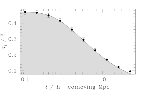
Figure 5.— The r.m.s. variation of the normalized transmissivity $\bar{f}/\langle\bar{f}\rangle(z)$ along skewers of different lengths. Points with error bars are for the 7 primary QSOs from Adelberger et al. (2003); the shaded curve is the prediction of equations 17 and 10. The observed values at the largest $l$ are unreliable due to uncertainties in the continuum fitting.

$\sigma_{V}^{2}$ is more difficult. It depends on the three-dimensional power-spectrum of the Lyman-$\alpha$ forest, which has not been measured due to a lack of close QSO pairs. A rough estimate of $\sigma_{V}^{2}$ can be obtained by scaling from $\sigma_{l}^{2}$, $\sigma_{V}^{2}\equiv\beta\sigma_{l}^{2}$, with $\beta$ a constant that can be estimated by assuming a shape for the powerspectrum and numerically integrating equations 10 and 11. According to McDonald (2003), the transmissivity powerspectra found in numerical simulations the high-redshift intergalactic medium have the form

$$P(k_{R},k_{z})\propto\Bigl{[}1+\beta k_{z}^{2}/k^{2}\Bigr{]}^{2}P_{L}(k)D(k_{R},k_{z})$$ (17)

where $k_{z}$ and $k_{R}$ specify the wavenumber in polar coordinates, $k^{2}\equiv k_{z}^{2}+k_{R}^{2}$, $P_{L}(k)$ is the linear powerspectrum of cold dark matter,

$$D(k_{R},k_{z})\equiv\exp\Bigl{[}\Bigl{(}\frac{k}{k_{nl}}\Bigr{)}^{\alpha_{nl}}-\Bigl{(}\frac{k}{k_{p}}\Bigr{)}^{\alpha_{p}}-\Bigl{(}\frac{k_{z}}{k_{v}(k)}\Bigr{)}^{\alpha_{v}}\Bigr{]},$$ (18)

and $k_{v}(k)\equiv(1+k/k_{v}^{\prime})^{\alpha^{\prime}_{v}}k_{v0}$. McDonald (2003) supplies values for the numerical constants in these equations appropriate to redshift $z\sim 2$. Adjusting his values slightly, to $\beta=1.73$, $k_{nl}=5.2$, $\alpha_{nl}=0.673$, $k_{p}=8.51$, $\alpha_{p}=1.14$, $k_{v0}=0.603$, $k_{v}^{\prime}=0.085$, $\alpha^{\prime}_{v}=0.432$, $\alpha_{v}=1.59$, and adopting a $\Gamma=0.2$ linear powerspectrum with a $P_{L}(k)\propto k^{0.95}$ long-wavelength limit (Bardeen et al. 1986), I find a transmissivity powerspectrum that correctly predicts both the observed dependence of $\sigma^{2}_{l}$ on $l_{z}$ at redshift $z=3$ (figure 5) and the observed one-dimensional transmissivity powerspectrum $P^{1D}(k_{z})\equiv 2\pi\int dk_{R}k_{R}P(k_{R},k_{z})$ at redshift $z=3$ (figure 6). This model powerspectrum is presumably a reasonable approximation to the true powerspectrum. Integrating it numerically in the following special cases of equation 11,

$$\sigma_{V}^{2} = \Bigl{(}\frac{1}{2\pi}\Bigr{)}^{2}\int dk_{R}\,dk_{z}k_{R}P(k_{R},k_{z})\Bigl{\{}\Bigl{[}\frac{\sin(k_{z}l_{z}/2)}{k_{z}l_{z}/2}\Bigr{]}^{2}\times$$ (19)

$$\quad\quad\quad\quad\quad\quad\quad\quad\Bigl{[}\frac{2J_{1}(k_{R}R)}{k_{R}R}\Bigr{]}^{2}\Bigr{\}}$$

or

$$\sigma_{V}^{2} = \Bigl{(}\frac{1}{2\pi}\Bigr{)}^{2}\int dk_{R}\,dk_{z}k_{R}P(k_{R},k_{z})\Bigl{\{}\Bigl{[}\frac{\sin(k_{z}l_{z}/2)}{k_{z}l_{z}/2}\Bigr{]}^{2}\times$$ (20)

$$\quad\quad\quad\quad\Bigl{[}\frac{2R_{o}J_{1}(k_{R}R_{o})-2R_{i}J_{1}(k_{R}R_{i}}{k_{R}(R_{o}^{2}-R_{i}^{2})}\Bigr{]}^{2}\Bigr{\}},$$

will produce an estimate of $\sigma_{V}^{2}/\sigma_{l}^{2}$ that is appropriate when $V$ is a cylinder of radius $R$ and height $l$ (equation 19) or a cylindrical annulus of inner radius $R_{i}$, outer radius $R_{o}$, and height $l$ (equation 20). Since the time-delay surface (§ 4) has rotational symmetry about the $z$ axis, cylindrical bins are a natural choice for the analysis.

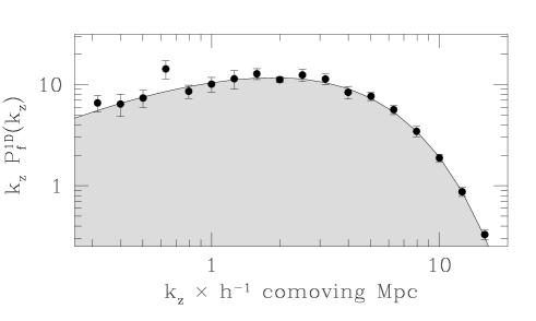
Figure 6.— The one-dimensional power-spectrum of the Lyman-$\alpha$ forest. Points are from the observations of McDonald et al. (2001); the shaded curve is the prediction of equation 17.

A more sophisticated treatment would take into account the changes to the power-spectrum that will accompany changes in the ionizing radiation intensity. That will likely require numerical simulations and is beyond the scope of this paper. However, since changes in the radiation field alter the neutral fraction but not the temperature of intergalactic gas (see § 2), they will have a stronger effect on the amplitude of the powerspectrum than on its shape. Amplitude-independent results (e.g., our estimate of $\sigma_{V}^{2}/\sigma_{l}^{2}$) may not be disastrously affected. Figure 7 presents some evidence in favor of this assertion. I converted published Lyman-$\alpha$ Voigt profile lists for the QSOs HS1946+7658 (Kirkman & Tytler 1997, $z=2.994$), Q0636+680, Q0956+122, Q0302-003, and Q0014+813 (Hu et al. 1995, $z=3.180$, 3.288, 3.294, 3.366) into a list of each QSO’s Lyman-$\alpha$ optical depth as a function of redshift, divided all the optical depths by a constant $b$ to mimic a change in the ionizing radiation intensity, then calculated the dependence of $\sigma_{l}$ on $l$ for various values of $b$. The top panel of figure 7 shows the result. The amplitude of $\sigma_{l}$ changes significantly with $b$, but its shape, which is sensitive to the shape of the powerspectrum, does not. This can be seen more clearly in the bottom panel, where the change in amplitude has been crudely removed by scaling each curve according to the relationship

$$\sigma_{l}\propto[1-\bar{f}(b)]^{0.43}$$ (21)

where $\bar{f}(b)$ is the mean transmissivity after dividing the actual optical depths by $b$. Once this scaling is removed, the $\sigma_{l}$ curves have nearly the same shape over the range $1\lower 2.15277pt\hbox{$\;\buildrel<\over{\sim}\;$}l\lower 2.15277pt\hbox{$\;\buildrel<\over{\sim}\;$}10h^{-1}$ comoving Mpc that is most important in our calculations.

Figure 7.— Top panel: $\sigma_{l}(l_{z})$ (the r.m.s. transmissivity fluctuation along a line segment of length $l_{z}$) recalculated after dividing the observed Lyman-$\alpha$ optical depths in the QSOs HS1946+7658, Q0636+680, Q0956+122, Q0302-003, and Q0014+813 by the number $b$ written next to each curve. Bottom panel: same as top, except the dependence of the amplitude on the mean transmissivity $\bar{f}(b)$ has been crudely removed by dividing each curve by $(1-\bar{f}(b))^{0.43}$. The differences in shape revealed by this panel are small over the distance range $1\lower 2.15277pt\hbox{$\;\buildrel<\over{\sim}\;$}l\lower 2.15277pt\hbox{$\;\buildrel<\over{\sim}\;$}10h^{-1}$ comoving Mpc that is most important to our analysis.

5.2. Commentary

It is worth considering the relative sizes of the terms in equation 16 before we move on. Suppose for concreteness that we are interested in measuring changes in the QSO’s luminosity over $10$Myr time-scales, so we have estimated the mean transmissivity in bins of depth $l_{z}\sim 1.5$ proper Mpc, and suppose further that the radius $R$ of our bins was chosen to fill the $40^{\prime}$ field-of-view of a mosaicked CCD camera, $R\sim 10$ proper Mpc at $z=3$ for $\Omega_{M}=0.3$, $\Omega_{\Lambda}=0.7$, $h=0.65$. In comoving units the bin has $R=26h^{-1}$ Mpc and $l_{z}=3.9h^{-1}$ Mpc, which implies $\sigma_{l}\simeq 0.17$ (figure 5, for $\bar{f}=0.67$), $\sigma^{2}_{l}/\sigma^{2}_{V}\simeq 20$, and consequently $\sigma_{V}\simeq 0.04$. Inserting these numbers into equation 16 leads to the two primary conclusions of this section:

(A) The spectra of the background objects do not need to be very good. The second and third terms in equation 16 contribute equally to the total uncertainty when the signal-to-noise ratio in a spectral segment of length $l_{z}\sim 3.9h^{-1}$ comoving Mpc ($\sim 7$Å) is ${\cal S}=\bar{f}/\sigma_{l}\sim 4$. Obtaining better spectra cannot change the total uncertainty by much. Random variations in the intergalactic matter density make the mean HI absorption $\bar{f}_{1}$ along a single sightline segment a poor indicator of the ionizing background $J_{\nu}$ and consequently there is no need to measure $\bar{f}_{1}$ with exquisite precision.

(B) The ultimate limit on our uncertainty is set by $\sigma_{V}$ and it is a limit that we will reach very quickly. For the example considered here, the first and second terms in equation 16 have the same size for $N=20$. Increasing $N$ further can reduce the second and third terms arbitrarily but not the total uncertainty. In practice one will want to obtain samples many times larger than $N=20$ to help address the possibility that the QSO’s radiation is beamed. As a result $\sigma_{V}$ will probably be the only significant contributor to $\sigma_{f}$ in realistic cases. The bottom panel of figure 2 shows that $\sigma_{V}$ is large enough to prevent us from detecting all but the coarsest changes in a QSO’s luminosity. We can do nothing about this. Only a small region of the universe is bathed in the light that the QSO emitted at one period in its history; the mean density in this region will stray from the global mean to the extent that inflation requires; the intensity of the QSO’s ionizing radiation cannot be measured if it influences the region’s mean HI absorption by less.

Although the numbers quoted above depend on our arbitrary choice for the bin size, neither $\sigma_{l}$ nor $\sigma_{V}$ is a strong enough function of $R$ or $l$ for the qualitative conclusions to change significantly as the bin size varies across its useful range. The change of variance with mean transmissivity (equation 21) might seem more important. If the QSO were bright enough to drive the mean transmissivity in a bin to $\bar{f}\sim 0.9$, for example, rather than the value $\bar{f}\sim 0.67$ assumed in the preceding three paragraphs, $\sigma_{l}$ would decrease to $0.10$, $\sigma_{V}$ would decrease to $0.02$, and one would find that spectra of slightly higher S:N were desirable. In practice, however, these high transmissivities are unlikely to be reached anywhere except very near the QSO, and here the decrease in $\sigma_{l}$ and $\sigma_{V}$ is largely offset by the small bin sizes that are required at small radii. This can be seen in the worked example of § 7, below.

One qualification should be added to my claim (A) that it is a waste of time to obtain high S:N spectra. That is necessarily true only if one is committed to using the mean transmissivity $\bar{f}$ as a probe of the radiation density $J_{\nu}$. At sufficiently high signal-to-noise ratios, however, other options are available. Consider an arbitrary function $g$ of the line-of-sight HI density that has variance $\sigma_{g}^{2}$ due to random fluctuations when the brightness $b\equiv J_{\nu}/J_{\rm bg}$ of the ionizing radiation field is kept constant. The random fluctuations in $g$ will prevent us from detecting relative changes in $b$ of order $\Delta{\rm ln}b\sim|d\,{\rm ln}b/d\,{\rm ln}g|\sigma_{g}/g$. If $g$ is the mean transmissivity $\bar{f}$ on a $3.9h^{-1}$ comoving Mpc line segment, which is the only possibility we have treated so far, then $d\,{\rm ln}b/d\,{\rm ln}g\sim 5$ (near $g=0.67$) and $\sigma_{g}/g\sim 0.26$, so the minimum detectable fluctuation in $b$ will have $\Delta{\rm ln}b\sim 1.3$. At high enough S:N it would be possible abandon $\bar{f}$ and adopt (say) the total HI column-density ${\cal N}$ along the same line segment as the probe of $b$. In this case, with $g={\cal N}$, we have $d\,{\rm ln}b/d\,{\rm ln}g\simeq-1$ and $\sigma_{g}/g\sim 6$, where $\sigma_{g}/g$ is the value that obtains among the 5 QSOs with $z\sim 3$ discussed at the end of § 5.1, so the minimum detectable fluctuation in $b$ has $\Delta{\rm ln}b\sim 6$. ${\cal N}$ is evidently far inferior to $\bar{f}$ as an estimator of $b$. A better choice, letting $g$ equal $n$, the number of detected Lyman-$\alpha$ forest lines on the segment, was advocated by Bajtlik, Duncan, & Ostriker (1988). If the column density distribution has the form $P(N_{\rm HI})\propto N_{\rm HI}^{-\alpha}$, then $d\,{\rm ln}b/d\,{\rm ln}g\simeq(1-\alpha)^{-1}$. Among the same 5 QSOs, $\sigma_{n}/n\simeq 0.5$ for line segments of length $3.9h^{-1}$ comoving Mpc, so the minimum detectable fluctuation in $b$ has $\Delta{\rm ln}b\sim 1$ for the observed slope $\alpha\sim 1.5$. Surprisingly, $n$ is only marginally better than $\bar{f}$ as an estimator of $J_{\nu}$. The mean transmissivity $\bar{f}$ along a segment of a low S:N galaxy spectrum can provide almost as strong a constraint on the intensity of the QSO’s radiation as a high S:N spectrum analyzed with the standard approach of Bajtlik, Duncan, & Ostriker (1988). It would be interesting to extend this analysis from $\sigma_{l}$ to the more relevant quantity $\sigma_{V}$. Since the ratio $\sigma_{l}/\sigma_{V}$ depends on the powerspectrum, and different estimators $g$ will have different powerspectra, it is not necessarily true that the best estimator for $\sigma_{l}$ will be best for $\sigma_{V}$. This method would be made far more powerful if one could finding an estimator that significantly reduces $\sigma_{V}$.

6. FEASIBILITY

The previous section glibly claimed that observational uncertainties can be made smaller than cosmic variance. This section considers the claim in more detail. The optimal depth for the spatial bins is $\sim 7$Å, corresponding roughly to 10 Myr time resolution (see § 8), and for the fields-of-view considered here the cosmic variance will consequently be $\sigma_{V}\sim 0.04$ (see §§ 5 and 7). This is the level to which we must reduce the observational uncertainty $\sigma_{\rm noise}$.

6.1. Signal

Reducing the random errors to the desired level $\sigma_{\rm noise}\sim 0.04$ is not much of a challenge. Figure 8 shows spectra with $\sim 10$Å resolution of three galaxies in the field SSA22a (Steidel et al. 2003) that were observed for $\sim 29000$s with the blue LRIS spectrograph (Steidel et al. 2004) on the Keck I telescope. The redshifts and AB-magnitudes of the galaxies ($z\sim 3.1$ and $G\sim 24.5$, respectively) are shown on the plot. The spectra are preliminary reductions that were selected more-or-less at random from the sample of Shapley et al. (2004, in preparation). These spectra have signal-to-noise ratios in the Lyman-$\alpha$ forest, for 7Å bins ($\sim 1.5$ proper Mpc), of around 5–6. Averaging together $\sim 10$ spectra of similar quality would reduce the random errors to the desired level. Roughly forty spectra would be required if the exposure time were 2 hours instead of 8.

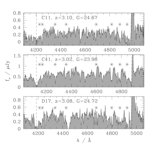
Figure 8.— Examples of the Lyman-$\alpha$ forest in the spectra of galaxies at redshift $z\sim 3$. The data were taken with LRIS-B (Steidel et al. 2004) and were generously provided by A. E. Shapley. Redshifts and AB magnitudes are indicated; the names (“C11” etc.) refer to the SSA22a catalog of Steidel et al. (2003). Asterisks mark the locations of the interstellar absorption lines discussed in figure 10, below. Dashed lines indicated the wavelengths of Lyman-$\alpha$ and Lyman-$\beta$ at the redshift of the galaxies’ interstellar absorption lines.

6.2. Continuum fitting

Systematic errors in the continuum fitting are a source of greater concern. We are interested not in a spectrum’s flux itself but rather in its implied Lyman-$\alpha$ transmissivity, which is the ratio between the observed flux and the continuum flux, i.e., the flux that would have been observed in the absence of Lyman-$\alpha$ absorption. The uncertainty in a bin’s mean transmissivity therefore has an additional term that arises from errors in the estimated continuum.

The size of these errors depends on the method that is used to estimate the continuum level. Traditional methods are poorly suited to the present case; they exploit the occasional presence of spectral regions with little Lyman-$\alpha$ absorption, and these regions are rare and difficult to recognize in noisy, low-resolution galaxy spectra. Several authors (e.g., Hui et al. 2001) have presented alternatives that are more useful to us. Particularly simple is the method of Croft (2004), in which the continuum level $c(\lambda)$ is estimated by simply smoothing each object’s spectrum and scaling appropriately: $c(\lambda)\simeq f_{50}(\lambda)/\bar{f}(z)$, where $f_{50}(\lambda)$ is the object’s Lyman-$\alpha$ forest spectrum smoothed by a Gaussian with $\sigma=50$Å and $\bar{f}(z)$ is the published mean transmissivity at redshift $z=\lambda/\lambda_{{\rm Ly}\alpha}-1$, which has been calculated by other authors from more-sophisticated continuum fits to the observed spectra of numerous bright QSOs.

Experimentation on the 7 QSOs with $z\sim 3$ in the sample of Adelberger et al. (2003) shows that transmissivities estimated with Croft’s (2004) approach and the traditional approach are very similar. Excluding the parts of the Lyman-$\alpha$ forest that fall on the QSOs’ Lyman-$\alpha$ and Lyman-$\beta$ emission lines, the correlation coefficient between the transmissivities estimated with the two approaches is $r\sim 0.96$–$0.98$. This implies that the r.m.s. difference between them, $(1-r^{2})^{1/2}\sigma_{l}$, is $\sim 0.03$–$0.05$ for 7Å bins with $\sigma_{l}\simeq 0.17$ (see Figure 5). Since galaxies’ and QSOs’ continua between Lyman-$\alpha$ and Lyman-$\beta$ are similarly featureless (see, e.g., figures 8, 9, and 10), errors in continuum fitting should introduce a similar uncertainty in galaxies’ Lyman-$\alpha$ forest transmissivities. Even if these errors were correlated from one galaxy to the next, and did not tend to cancel in the averaged transmissivity in each spatial bin, their size would be no larger than the cosmic variance. In practice continuum errors from the Croft (2004) approach should cancel significantly, however. They arise, to a large extent, because the Lyman-$\alpha$ forest is not completely uniform on $\sim 100$Å scales and any deviations from uniformity are incorrectly interpreted as features of the continuum. The resulting r.m.s. continuum error averaged over a spatial bin can be calculated with the approach of § 5:

$$\sigma_{\rm cont}\simeq\biggl{[}\frac{N-1}{N}{\sigma^{\prime}}_{V}^{2}+\frac{1}{N}{\sigma^{\prime}}_{l}^{2}\biggr{]}^{1/2}$$ (22)

where ${\sigma^{\prime}}_{V}^{2}$ and ${\sigma^{\prime}}_{l}^{2}$ are given by equations 11 and 10 with $\sin(k_{z}l_{z}/2)/(k_{z}l_{z}/2)$ replaced by $\exp[-k_{z}^{2}\sigma_{z}^{2}/2]$, where $\sigma_{z}$ is the comoving distance corresponding to the $50$Å smoothing length. Since $\sigma_{z}\gg l_{z}$, ${\sigma^{\prime}}_{V}^{2}$ will be smaller than $\sigma_{V}^{2}$, ${\sigma^{\prime}}_{l}^{2}$ will be smaller than $\sigma_{l}^{2}$, and the uncertainty from this source of continuum errors will never dominate the total uncertainty. This is true even in the low signal-to-noise limit, since in this case the uncertainty in the smoothed continuum will be dwarfed by the uncertainty in a single $\sim 7$Å bin.

Figure 9.— Comparison of galaxy and QSO continua in the Lyman-$\alpha$ forest region. The top panel shows the gravitationally lensed galaxy MS1512-cB58 (Pettini et al. 2002); the bottom panel shows the QSO Q1623 KP78 (Adelberger et al. 2004, in preparation). Both spectra were taken with the same instrument, though the signal-to-noise ratio for the bright QSO is significantly higher. Asterisks in the top panel mark the locations of the interstellar absorption lines discussed in figure 10, below.

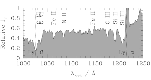
Figure 10.— Mean absorption vs. wavelength for galaxies at redshift $z\sim 3$. The shaded curve shows the mean spectrum of 811 galaxies at $z\sim 3$; the data are taken from Shapley et al. (2003). Lyman-$\alpha$ forest fluctuations cancel out in this average, producing a smooth shelf with mean transmissivity $\bar{f}\sim 0.67$ between Lyman-$\alpha$ and Lyman-$\beta$. Absorption lines in this shelf are produced by material intrinsic to the galaxies. This interstellar absorption can be safely ignored when its rest-frame equivalent width is less than $\sim 0.3$Å(see text). Stronger lines have been marked with vertical labels naming the ion responsible for the absorption. Data at these wavelengths should be excluded when calculating the mean transmissivity in different spatial bins. Note that the resolution of this spectrum ($\sim 12$Å) is somewhat lower than the 7Å resolution advocated in the text.

6.3. Interstellar absorption lines

Although galaxies’ continua appear to be mostly featureless between Lyman-$\alpha$ and Lyman-$\beta$, there are some important exceptions: at a handful of wavelengths the galaxies’ interstellar absorption lines are too strong to be ignored. These wavelengths are apparent in figure 10, which shows average observed absorption in region between Lyman-$\alpha$ and Lyman-$\beta$ in a sample of 811 Lyman-break galaxies (Shapley et al. 2003). Since the r.m.s. variation in Lyman-$\alpha$ forest transmissivity in 7Å bins is $\sigma_{l}\simeq 0.17$ (Figure 5), interstellar absorption lines will have a non-negligible effect on the estimated transmissivity if their rest-frame equivalent width exceeds $7$Å$\times\sigma_{l}/(1+z)\simeq 0.3$Å. In the mean spectrum of Shapley et al. (2003) there are 7 such lines between Lyman-$\alpha$ and Lyman-$\beta$. The existence of these interstellar absorption lines will not have a disastrous effect on the analysis, since each background galaxy will lie at a slightly different redshift, but one might as well eliminate their effect completely by masking the relevant portions of the spectrum. This will reduce the effective number of background galaxies by too modest an amount to significantly alter the significance of any conclusions.

7. SYNTHESIS

We can now estimate how easily we will be able to detect ionization gradients produced by changes in a QSO’s luminosity. This section works through the details for a single case, an isotropically radiating QSO of ($t=0$) magnitude $m_{912}=18$ whose ionizing luminosity varied with time according to the curve $L(t)$ shown in the top panel of figure 11. An $\Omega_{M}=0.3$, $\Omega_{\Lambda}=0.7$, $h=0.65$ cosmology with the uniform ionizing background of equation 2 will be assumed throughout this section.

Figure 11.— Top panel: the QSO’s ionizing luminosity as a function of time. This curve, generated for the example of section 7, is not intended to be a realistic model of a QSO’s output. It features were chosen to illustrate a number of points made in the text. Bottom panel: the recovered mean transmissivity in bins whose edges align with contours of the time-delay surface. Points mark the mean transmissivity calculated from figure 12; error bars show the $1\sigma$ range that would be observed if figure 12 included cosmic variance, the dominant noise source. The solid curve shows the mean transmissivity than would have been observed if the QSO’s luminosity were constant, $L(t)=L(0)$. The dotted curve shows the mean transmissivity in the primed “control” bins (figure 12); it differs from the solid line due to the increase in the QSO’s luminosity from $t=0$ to $t=-10$, though this effect would presumably be removed by a maximum likelihood fit of the data to a surface. Decreases of the luminosity to 0 and subsequent increases back to $L(0)$ can be detected with moderate significance if they happened within the interval $-50\lower 2.15277pt\hbox{$\;\buildrel<\over{\sim}\;$}t\lower 2.15277pt\hbox{$\;\buildrel<\over{\sim}\;$}0$ Myr. Only extremely large increases in the QSO’s luminosity can be detected at earlier times.

According to equation 6, the radiation intensity as a function of position in the observed frame (i.e., the radiation intensity that was present when the photons from the background sources passed through each point) is

$$J(R,z)=\Bigl{[}1+\frac{L(t_{I}(R,z))}{L(0)}\Bigl{(}\frac{r_{\rm eq}}{r}\Bigr{)}^{2}\Bigr{]}J_{\rm bg}$$ (23)

where $t_{I}(R,z)$ and $r_{\rm eq}$ are given by equations 7 and 8. The left panel of figure 12 shows this function for $r_{\rm eq}=8.27$ proper Mpc, which is appropriate to the QSO described in the preceding paragraph. Since the ionization and recombination times (§ 2) are short compared to the time for significant changes in $L(t)$, the neutral fraction will be inversely proportional to $J(R,z)$, and the mean corresponding transmissivity $f(R,z)$ can be derived from the curve shown in the top panel of figure 2. The result is shown in the right panel of figure 12. The panel shows the mean transmissivity that would be observed if one averaged results from many identical QSOs; the actual transmissivity surrounding a single QSO would have significant variations about this mean, due primarily to random fluctuations in the density of intergalactic matter.

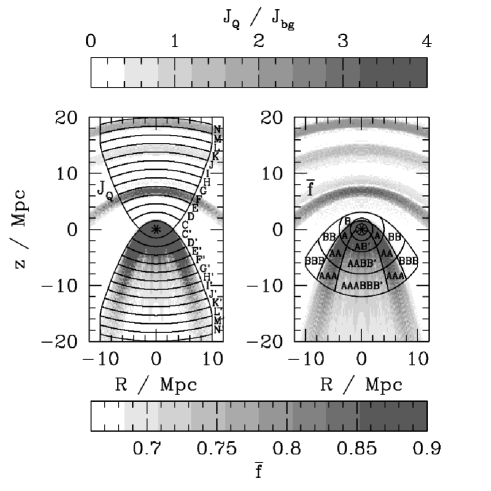
Figure 12.— Left panel: variations in the intensity of ionizing radiation in the observed frame for a QSO at redshift $z=3$ with $m_{912}=18$ that has the history of outbursts shown in figure 11. Also shown are sample bins used in the analysis at larger lookback times. Right panel: variations in the expected mean transmissivity implied by the radiation intensity of the left panel. The mean transmissivity would hew to these values only if results from numerous identical QSOs were averaged. A more realistic single realization would show large fluctuations in the transmissivity due to random variations in the density of intergalactic matter. The labeled regions surrounding the QSO are sample bins for the analysis at smaller lookback times.

Changes in the QSO’s ionizing luminosity could be detected in various ways, but for now I will assume that one is aiming to detect the changes by looking for differences in the mean transmissivity $\bar{f}_{\rm bin}$ among bins whose edges trace contours of the time delay surface $t_{I}(R,z)$. One set of such bins is shown in the left panel of figure 12. Also indicated are symmetrically distributed “control” bins. These bins have shapes identical to the others, but are located on the opposite side of the QSO, in a region that is illuminated by the QSO’s radiation at short time delays $0>t>-10$ Myr. The mean transmissivity in these bins provides an indication of how the mean transmissivity for $z>0$ would vary with position if the QSO’s luminosity were always equal to its observed ($t=0$) value(§ 4). Note that the requirement $t>-10$ Myr for the control bins limits the size of their partner bins at smaller radii.

Our ability to detect changes in the QSO’s luminosity will depend on the uncertainty in the binned transmissivity $\bar{f}_{\rm bin}$. For a reasonable number of background sources ($\;\buildrel>\over{\sim}\;$ few dozen) this uncertainty will be nearly equal to the cosmic variance $\sigma_{V}$ (§ 5). As discussed in § 5, the size of $\sigma_{V}$ can be roughly estimated by (1) approximating each bin as a cylinder of radius $R_{\rm bin}$ and depth $l_{\rm bin}$, (2) calculating r.m.s. transmissivity fluctuation along a skewer of length $l_{\rm bin}$ by interpolating from figure 5 and scaling according to the local expected transmissivity $f(R,z)$ with equation 21, and (3) multiplying by $\beta^{1/2}$, where $\beta(R_{\rm bin},l_{\rm bin})\equiv\sigma^{2}_{V}/\sigma^{2}_{l}$ is a constant that can be determined for each bin by numerically integrating equations 10, 19, and 17. The bottom panel of figure 11 shows the expected mean transmissivity in each bin along with the estimated $1\sigma$ uncertainty calculated in this way.

The main conclusions from figure 11 are (1) that only large changes in the QSO’s luminosity will leave an imprint on the IGM that is easily detectable with this approach, and (2) that the minimum size of a detectable luminosity difference increases rapidly towards earlier times. These conclusions are easier to apprehend in figure 13, which shows the 10-Myr moving-average magnitude $\bar{m}_{912}$ a QSO would need to have had at various lookback times to for its sudden death (or revival) to leave a detectable fossil record in the spectra of background galaxies. Measuring changes in a QSO’s luminosity will be difficult for $t\lower 2.15277pt\hbox{$\;\buildrel<\over{\sim}\;$}-50$ Myr and nearly impossible for $t\lower 2.15277pt\hbox{$\;\buildrel<\over{\sim}\;$}-100$ Myr. At smaller time delays the prognosis is good.

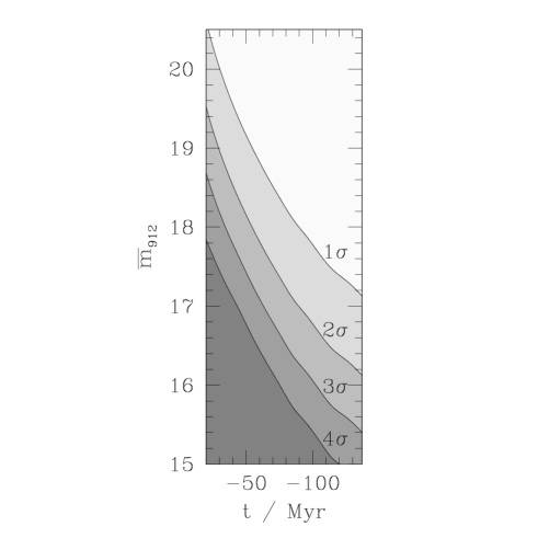
Figure 13.— The $10$Myr running-average luminosity required at various lookback times for the flux in the corresponding $10$Myr bin to be $N\sigma$ above the background level. Luminosity changes among even the brightest QSOs will be difficult to detect at moderate significance for $t\lower 2.15277pt\hbox{$\;\buildrel<\over{\sim}\;$}-100$ Myr.

As $t\to 0$, the shape of the time-delay contours becomes increasingly incompatible with the goal of having symmetrical control bins. For $-20\lower 2.15277pt\hbox{$\;\buildrel<\over{\sim}\;$}t\lower 2.15277pt\hbox{$\;\buildrel<\over{\sim}\;$}0$ the best approach may be to abandon the binning altogether and simply find the maximum likelihood fit of the data to an appropriate surface. To give some indication of the uncertainty in the radiative history that would result, however, I will continue a binned analysis with the bins shown in the right panel of figure 12. The outermost bins ($B$–$BBB$) enclose regions with time delays $-20<t<-10$ Myr, the middle bins ($A$–$AAA$) enclose $-10<t<-3.5$ Myr, and the innermost ($AB^{\prime}$ etc.) enclose $-3.5<t<0$ Myr. A complication for these small time delays is that a region with fixed $t$ has a wide range of distances $r$ to the QSO. Variations in $\bar{f}$ due to changes in $1/r^{2}$ could obscure the variations of interest from changes in the QSO luminosity $L(t)$. My approach in this simplified analysis is to divide each time-delay region into a number of bins with similar values of $r$ (e.g., bins $B$, $BB$, and $BBB$ for $-20<t<-10$ Myr). Figure 14 shows the mean transmissivity within each of these bins. The uncertainty in the bins was calculated by approximating them as cylinders ($B$, $AB^{\prime}$, $AABB^{\prime}$, $AAABBB^{\prime}$) or cylindrical annuli ($A$–$AAA$, $B$–$BBB$) with the same volume and roughly the same shape; the expected variance does not depend sensitively on the details of this approximation.

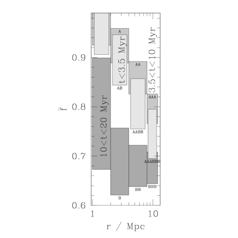
Figure 14.— The mean transmissivity and its uncertainty in the bins shown in the right panel of figure 12. Bins with the lightest shading are bathed in light emitted by the QSO at $-3.5{\rm Myr}<t<0$; bins with medium shading by light emitted at $-10<t<-3.5$Myr; bins with darkest shading by $-20<t<-10$Myr. The height of the bins corresponds to the mean transmissivity $\pm 1\sigma$. Bin names in this figure correspond to those in figure 12. Bins with $1<r<2$Mpc are unlabeled in figure 12 for clarity. At fixed time delay, $\bar{f}$ declines with radius due to the $1/r^{2}$ decline in flux from the QSO. Comparing $\bar{f}$ radius by radius clearly reveals the decline in $L(t)$ (figure 11) from $-10{\rm Myr}<t<0$ to $-20<t<-10$Myr. The increase from $-3.5{\rm Myr}<t<0$ to $-10<t<-3.5$Myr would not be easy to detect; a decrease during the same times would have been detected with high significance.

With these bins, the decrease in $L(t)$ from $-10<t<0$ Myr to $-20<t<-10$ Myr is detected with some significance at each radius and with high significance when the results from different radii are combined. If the decrease had happened at an earlier time $-10<t\lower 2.15277pt\hbox{$\;\buildrel<\over{\sim}\;$}-3.5$ Myr it would have been detected with higher significance still. Instead the luminosity increased from $-3.5{\rm Myr}<t<0$ to $-10<t\lower 2.15277pt\hbox{$\;\buildrel<\over{\sim}\;$}-3.5$. As the plot shows, increases in the luminosity at small look-back times are much harder to detect than decreases, since the sensitivity of $\bar{f}$ to $J_{Q}$ falls as $\bar{f}\to 1$ (figure 2). Fortunately decreases must be far more likely than increases: QSOs with $m_{912}=18$ lie on the steep bright-end of the luminosity function.

8. LIMITS TO THE TIME RESOLUTION

In the previous sections the data were placed into spatial bins whose depth $l_{z}=1.5$ Mpc gave us sensitivity to luminosity fluctuations time-scales of $10$ Myr or greater. Ideally one would be able to detect fluctuations on any time scale. Could we have achieved significantly better time resolution by placing the data in bins with smaller $l_{z}$? The answer is no; this section explains why.

If cosmic variance were the only problem, the bin depth $l_{z}$ could be made arbitrarily small. $\sigma_{V}$ (equation 19) is almost independent of $l_{z}$ for $l_{z}\ll R$, the case of interest, and so a bin that is infinitesimally thin will have nearly the same cosmic variance as the adopted bins with $l_{z}=1.5$ proper Mpc.

Unfortunately the ability to obtain reasonably accurate estimates of the mean transmissivity in infinitesimally thin bins is not the same as the ability to measure changes in the QSO’s luminosity that happened on arbitrarily short time scales. Our estimate of a gas element’s longitudinal separation $z$ from the QSO will be inaccurate for two reasons: (1) we will not know the precise redshift of the QSO, and (2) our $z$ positions are derived from redshifts and will be distorted from their true values by peculiar velocities. As a result the time delay to the element is uncertain. When the time delays to different elements are uncertain, we cannot combine elements with exactly the same delays into one bin; the various elements that make up a single bin will inevitably have a range of time delays. The minimum range of time delays in a bin is what limits our time resolution. The remainder of the section considers this limit in more detail.

8.1. Uncertainty in the QSO redshift

If the QSO’s redshift is measured from the CIV emission line, the uncertainty in its systemic recession velocity will be $\sigma_{v}\simeq 510{\rm km}\,{\rm s}^{-1}$ (Richards et al. 2002), which corresponds to a positional uncertainty of $\sigma_{z}\simeq 1.75h_{65}^{-1}$ proper Mpc at $z=3$ for $\Omega_{M}=0.3$, $\Omega_{\Lambda}=0.7$. The uncertainty can be reduced to $0.9h_{65}^{-1}$ proper Mpc (i.e., $270{\rm km}\,{\rm s}^{-1}$) if MgII is used instead (Richards et al. 2002), and to $0.3h_{65}^{-1}$ proper Mpc (i.e., $80{\rm km}\,{\rm s}^{-1}$) if [OIII] is used (Vrtilek & Carleton 1985). Radio observations of molecular emission lines could presumably reduce $\sigma_{z}$ even further, but this is unlikely to benefit us much. The time resolution achievable with $\sigma_{z}=0.3$ proper Mpc is $t\sim 2\sigma_{z}/c\sim 2$ Myr, and other effects prevent us from obtaining a resolution even this coarse.

8.2. Thermal motions

A firm lower limit to the time resolution is set by the thermal motions of the $20000$ K intergalactic gas. The intergalactic hydrogen at a particular true $z$ position will have an rms range of apparent $z$ position of $\sigma_{z}=(kT/m_{H})^{1/2}/H\simeq 0.04$ proper Mpc for $\Omega_{M}=0.3$, $\Omega_{\Lambda}=0.7$, $h=0.65$. We will not be able to measure changes in the QSO’s luminosity that happen much more rapidly than the corresponding time scale $t\sim 2\sigma z/c\sim 0.3$ Myr. This is unlikely to be the limiting factor in the analysis.

8.3. Streaming towards the QSO

The effect of larger-scale peculiar velocities is more severe. First there is the average streaming motion towards the QSO, which can be crudely estimated as follows. If the scale dependence of QSOs’ bias $b$ is weak, then the mean matter overdensity at a distance $r$ from a QSO will be roughly $\delta(r)=\xi_{Q}(r)/b$, where $\xi_{Q}$ is the correlation function of QSOs. According to Croom et al. (2002), a correlation function of the form $\xi_{Q}(r)=(r/r_{0})^{-\gamma}$, $r_{0}\simeq 8.4h^{-1}$ comoving Mpc, $\gamma\simeq 1.56$ is appropriate for the brightest QSOs at any redshift. The variance of QSO number density in cells of radius $r_{\rm cell}=8h^{-1}$ comoving Mpc is therefore $\sigma_{Q}^{2}=72(r_{0}/r_{\rm cell})^{\gamma}/[(3-\gamma)(4-\gamma)(6-\gamma)2^{\gamma}]\simeq 1.3$, (Peebles 1980 eq. 59.3), which implies a QSO bias at $z=3$ of $b\simeq 4.5$ if $\Omega_{M}=0.3$, $\Omega_{\Lambda}=0.7$, and the rms linear matter-density fluctuation in $r=8h^{-1}$ Mpc spheres at $z=0$ is $\sigma_{8}=0.9$. Integrating over the correlation function shows that the mean matter overdensity within a comoving radius $r_{c}$, $\bar{\delta}(r_{c})$, is roughly

$$\bar{\delta}(r)\simeq\frac{3r_{c}^{-\gamma}}{(3-\gamma)br_{0}^{-\gamma}}.$$ (24)

Now the proper radius $r_{p}$ of a spherically symmetric region with mean interior overdensity $\bar{\delta}$ evolves according to

$$\frac{\dot{r}_{p}}{r_{p}}=H-\frac{1}{3(1+\bar{\delta})}\frac{d\bar{\delta}}{dt}$$ (25)

where $H(t)$ is the Hubble parameter. This follows from the fact that concentric shells of matter do not cross until just before final collapse. Adopting the spherical Zeldovich approximation for simplicity, the linear overdensity density $\bar{\delta}_{L}$ will be related to the true overdensity through $1+\bar{\delta}\sim(1-\bar{\delta}_{L}/3)^{-3}$, which reduces equation 25 to

$$\frac{\dot{r}_{p}}{r_{p}}=H\Bigl{[}1+f-f\,\bigl{(}1+\bar{\delta}(r_{p})\bigr{)}^{1/3}\Bigr{]},$$ (26)

and shows that

$$\Delta z=f\frac{z}{(R^{2}+z^{2})^{1/2}}\Bigl{[}1-\bigl{(}1+\bar{\delta}(r_{p})\bigr{)}^{1/3}\Bigr{]},$$ (27)

is the rough proper distance between the a volume element’s true position $(R,z)$ and the position we that we erroneously infer from assuming that it is at rest with respect to the Hubble flow. Here $f\equiv d{\rm ln}D/d{\rm ln}a\simeq\Omega_{M}^{0.6}(z)$ where $D$ is the linear-growth factor and $a$ is the scale factor of the universe. Figure 15 shows $\bar{\delta}$ and $\Delta z$ as a function of distance.

Figure 15.— The mean interior overdensity (solid line) and approximate infall velocity (dashed line) as a function of distance from a bright QSO at $z=3$. The infall velocity is expressed as $\Delta r/r\equiv(r_{\rm apparent}-r_{\rm true})/r_{\rm true}$, the relative shift in an object’s position that the infall velocity would produce if the velocity were directed exactly towards the observer. The infall velocity is estimated with a simple version of the Zeldovich approximation that becomes inaccurate for $\bar{\delta}\gg 1$; see text.

By itself the net streaming towards the QSO is not a major problem, at least for $r\lower 2.15277pt\hbox{$\;\buildrel>\over{\sim}\;$}5h^{-1}$ comoving Mpc. Its primary effect is to make absorbing gas appear to be closer to the QSO than it actually is. Although this produces a slight systematic error in the lookback time assigned to each volume element, the error can be corrected to a large degree with simple formulae such as equation 27, and in any case slight inaccuracies in the times assigned to the $x$ axis of figure 11 would not diminish its scientific value by much.

8.4. Random peculiar velocities

More troubling are random deviations around the net streaming motion. As a result of them, the gas that is illuminated by the QSO’s luminosity at time $t$ will lie on a complicated surface that wanders randomly around the parabolic time-delay surface shown in figure 3. Since particles maintain their linear velocities long after the density field itself has left the linear regime, and since most of intergalactic space should be occupied by low density (i.e., uncollapsed) gas that is not far from the linear regime, linear perturbation theory should provide a rough estimate of the typical size of these excursions. Let $\sigma_{v_{z}}({\mathbf{r}})$ be the rms difference in the $z$ comoving peculiar velocities of two points separated by the vector ${\mathbf{r}}$. In the linear regime the Fourier transform $\tilde{\mathbf{v}}({\mathbf{k}})$ of the comoving peculiar-velocity field ${\mathbf{v}}({\mathbf{r}})$ is related to the Fourier transform $\tilde{\delta}({\mathbf{k}})$ of the comoving density field $\delta({\mathbf{r}})$ through $\tilde{\mathbf{v}}({\mathbf{k}})=-iHf\tilde{\delta}({\mathbf{k}}){\mathbf{k}}/k^{2}$, (e.g., Peebles 1980 equation 27.22) where $H$ is the Hubble parameter and $f\simeq\Omega_{M}^{0.6}(z)$. Convolving $v_{z}({\mathbf{r}})$ by the sum of a positive delta function at ${\mathbf{r}^{\prime}}/2$ and a negative delta function at $-{\mathbf{r}^{\prime}}/2$ produces a new random field whose value at each point is equal to the $z$-velocity difference between the points ${\mathbf{r}^{\prime}}/2$ and $-{\mathbf{r}^{\prime}}/2$. The variance of this field is equal to $\sigma_{v_{z}}^{2}({\mathbf{r}})$, which can therefore be written, according to equation 12, as

$$\sigma_{v_{z}}^{2}({\mathbf{r}})=\frac{H^{2}f^{2}}{2\pi^{3}}\int d^{3}k\,\frac{k_{z}^{2}}{k^{4}}P_{L}({\mathbf{k}})\sin^{2}\Bigl{(}\frac{{\mathbf{k}}\cdot{\mathbf{r}}}{2}\Bigr{)}.$$ (28)

Expressing $\sigma_{v_{z}}^{2}({\mathbf{r}})$ in terms of one-dimensional integrals by converting to spherical coordinates and integrating over solid angle, one finds

$$\sigma_{v_{z}}^{2}({\mathbf{r}})=2[\psi_{\|}(0)-\psi_{\|}(r)\cos^{2}(\theta)-\psi_{\bot}(r)\sin^{2}(\theta)],$$ (29)

where $\theta$ is the angle between ${\mathbf{r}}$ and the $z$ axis,

$$\psi_{\|}(r)\equiv\frac{H^{2}f^{2}}{2\pi^{2}}\int_{0}^{\infty}dk\,P_{L}(k)\Biggl{[}\frac{\sin(kr)}{kr}-2\Biggl{(}\frac{\sin(kr)}{(kr)^{3}}-\frac{\cos(kr)}{(kr)^{2}}\Biggr{)}\Biggr{]}$$ (30)

and

$$\psi_{\bot}(r)\equiv\frac{H^{2}f^{2}}{2\pi^{2}}\int_{0}^{\infty}dk\,P_{L}(k)\Biggl{[}\frac{\sin(kr)}{(kr)^{3}}-\frac{\cos(kr)}{(kr)^{2}}\Biggr{]}.$$ (31)

This is a special case of a result derived by Górski (1988). If the wavenumbers in the integrals are comoving, as is the convention, the rms error in comoving $z$ separation due to peculiar velocities is $\sigma_{z}({\mathbf{r}})=\sigma_{v_{z}}({\mathbf{r}})/H$. Inserting the $\Gamma=0.2$ linear powerspectrum of Bardeen et al. (1986) into these equations, normalizing to $\sigma_{8}=0.9$ at redshift $z=0$ (i.e., to $\sigma_{8}\simeq 0.29$ at $z=3$, appropriate for $\Omega_{M}=0.3$, $\Omega_{\Lambda}=0.7$), and integrating numerically, I find the values of $\sigma_{z}$ shown in figure 16.

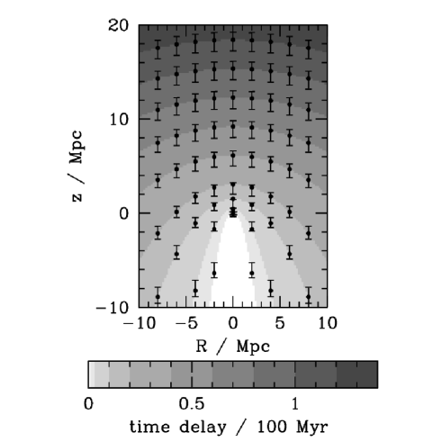
Figure 16.— The peculiar velocity field. Peculiar velocities add random offsets to the apparent $z$ positions of intergalactic gas and systematically shift them towards the QSO. Black points mark the true spatial positions of selected intergalactic volume elements; error bars show the expected $1\sigma$ range of each volume element’s apparent position. The mean offsets were calculated with equation 27 and the sizes of the ranges with equation 29. Contours in the background show the time delay to each position, starting with $1$, $3$, $10$, $20$ Myr and increasing in steps of 20 Myr thereafter. Because of peculiar velocities, gas with a range of time delays is mixed together in any spatial bin that is defined in the observed (redshift-space) frame. This limits the time resolution of the method. For time delays greater than $\sim 20$ Myr, the time resolution is limited to $\lower 2.15277pt\hbox{$\;\buildrel>\over{\sim}\;$}10$ Myr. At very small time delays the resolution is far better. Peculiar velocities are unlikely to make material with a delay of $\sim 1$ Myr appear to have a delay of 3 Myr, for example, so we should be able to use the method to detect QSO lifetimes of order 1 Myr even though we will not be able to distinguish a life time of 30 Myr from one of 31 Myr.

8.5. Upshot

Random peculiar velocities are likely to be the dominant source of uncertainty in a volume element’s distance to the QSO. The uncertainty in the element’s proper $z$ position is $\sigma_{z}\sim 1$ proper Mpc, which corresponds to a time-scale of $t\sim 2\sigma_{z}/c\sim 7$ Myr. It might be possible, with very high signal-to-noise spectra for a very large number of background sources, to trace and correct these distortions to the time delay surface. A number of interesting applications would then be possible. With current technology, however, we will have accept that the mean transmissivity in any bin we devise will be sensitive to the QSO’s luminosity over a $\sim 10$ Myr range of lookback times. Time resolution significantly better than this does not appear to be achievable.

9. SUMMARY AND DISCUSSION

This paper showed that changes over time in the luminosity of a QSO at redshift $z\sim 3$ will produce ionization gradients in the IGM and alter the Lyman-$\alpha$ forest absorption spectra of background galaxies in an observable way. Because the density of detectable galaxies (${\cal R}\lower 2.15277pt\hbox{$\;\buildrel<\over{\sim}\;$}25$) at $z\sim 3$ is high, $\sim 1\,{\rm arcmin}^{-2}$, their absorption spectra can provide a detailed view of the ionization gradients. If an isotropically radiating QSO has an AB magnitude at 912Å of $m_{912}=18$, significant decreases in its luminosity at larger look-back times will be detectable if they happen $1\lower 2.15277pt\hbox{$\;\buildrel<\over{\sim}\;$}t\lower 2.15277pt\hbox{$\;\buildrel<\over{\sim}\;$}50$ Myr before the time of observation. The time limits expand for brighter QSOs and shrink for fainter. Increases in the QSO’s luminosity over this time period will be harder to detect than decreases, but since $m_{912}=18$ corresponds to the steep bright end of the QSO luminosity distribution, they must be much rarer. § 7 sketches out the method and presents the uncertainties for a simulated QSO with known radiative history $L(t)$; the section is aimed at those who want more detail but are reluctant to read the entire paper.

The method gives us sensitivity to changes in a QSO’s luminosity over a useful range of times. Statistical arguments mentioned in the introduction show that QSOs must change their luminosities significantly on time-scales $t\lower 2.15277pt\hbox{$\;\buildrel<\over{\sim}\;$}100$ Myr. If these changes happen on time-scales $t\lower 2.15277pt\hbox{$\;\buildrel<\over{\sim}\;$}0.1$–1 Myr, a handful of QSOs in large (SDSS-sized) samples will show major brightness changes from one decade or century to the next (Martini & Schneider 2003). The method I have described cannot detect luminosity changes that happen on time-scales so short (§ 8), but is sensitive changes throughout the rest of the allowed range ($1\lower 2.15277pt\hbox{$\;\buildrel<\over{\sim}\;$}t\lower 2.15277pt\hbox{$\;\buildrel<\over{\sim}\;$}100$ Myr). Taken together, the two methods will be able to pin down the typical QSO lifetime in a robust and direct way.

A number of other authors (e.g., Crotts 1989; Dobrzycki & Bechtold 1991; Moller & Kjaergaard 1992; Fernández-Soto et al. 1995; Liske & Williger 2001; Jakobsen et al. 2003; Schirber, Miralda-Escudé, & McDonald 2004; Croft 2004) have attempted to measure QSO lifetimes with a similar approach. Their results were ambiguous. The reason is that they used the absorption lines in a single background QSO (or, in some cases, a handful) to search for ionization gradients around the foreground QSO. When the QSO pair had a small projected separation, the analyses were confused by the high densities and large peculiar velocities near the foreground QSO (see, e.g., figure 15); when the projected separation was large the foreground QSO’s weak effect on the IGM could not stand out above the cosmic variance. This paper’s method sidesteps these difficulties by using numerous faint galaxies rather than a small number of bright QSOs as the background sources. As shown in § 5, the signal-to-noise ratio of the background objects’ spectra does not affect the final result by much, but the number of background sources does. Choosing galaxies as the background sources is therefore the sensible approach. With numerous background sources, the weak effect of a QSO on distant intergalactic matter can be detected with reasonable significance, the complicated region closest to the QSO can be ignored altogether, and the peculiar velocity and density gradients at slightly larger distances can be compensated by comparing to the amount of Lyman-$\alpha$ absorption in the large “control region” that is illuminated by light emitted by the QSO at $t\sim 0$ (§ 4). The approach I have described should therefore be a significant improvement over previous work.

Observers who would like to apply this approach in practice should be aware that the optimal proper size of the observed region can be very different from the naive guess $ct_{\rm max}$ with $t_{\rm max}$ the maximum time delay of interest. As $t_{\rm max}\to 0$ intergalactic absorption at radii $R\gg ct_{\rm max}$ becomes increasingly important for the analysis, as figures 3 and 14 show. Two results derived in § 5 are also relevant. They are discussed more fully in § 5.2, but may be summarized as follows: (A) Galaxy spectra with $S$:$N\sim 4$ per 7Å bin will be sufficient for measuring the QSO’s radiative history with the stated precision. Obtaining better spectra will not improve the result by much. (B) Cosmic variance places a fundamental limit on the accuracy of the method. Only a small part of the universe is bathed in the light that the QSO emitted at a particular moment in its history, and the HI content of this region will stray from the global average for reasons that have nothing to do with the luminosity of the QSO. The only detectable luminosity changes are those large enough to alter the intergalactic HI content by more than its intrinsic random fluctuations $\sigma_{V}$. A corollary is that the number of background sources does not need to be incredibly high; one needs only enough to measure the mean transmissivity of a region with a precision similar to $\sigma_{V}$, and this is easily achieved with spectra of a few dozen galaxies (but see below).

I have neglected an important complication in the discussion so far. It is possible that the QSO’s ionizing radiation will not emerge isotropically but will instead be focused into a bipolar beam with opening angle $\alpha\sim 90^{\rm o}$ (Barthel 1989). If the beam were pointed towards earth there would be almost no effect on the analysis (see figure 12), but in the typical case the intergalactic volume that is affected by the QSO’s radiation will be only $\sim 30$% as large as I have assumed. This will increase the uncertainty in the results. Shrinking the radius of one of our idealized cylindrical bins (§§ 5 and 7) until it contains only $30$% of its previous volume will increase its uncertainty due to cosmic variance, $\sigma_{V}$, by a factor of $\sim 1.5$. If cosmic variance is still the dominant source of noise in the smaller bins, the error bars in the $\bar{f}$ vs. $t$ curve will increase by a similar factor. Fortunately this is not enough to prevent us from detecting changes in the QSO’s luminosity for $-50{\rm Myr}\lower 2.15277pt\hbox{$\;\buildrel<\over{\sim}\;$}t$ (figure 11). Moreover, even with the enlarged error bars it should be easy to distinguish intergalactic volumes that are illuminated by the QSO’s ionizing radiation from neighboring regions with transmissivities close to the global mean of $\bar{f}\sim 0.67$, at least at small radii where the QSO’s radiation is most intense (see, e.g., figure 14, which shows that the QSO’s influence at small radii should be detected with high significance). This statement is independent of the QSO’s radiative history as long as it has been shining for more than $\sim 10$ Myr, since so large a volume is (potentially) illuminated by light emitted at $-10{\rm Myr}<t<0$. If one were still worried about the possibility of beaming, QSOs could be chosen for study only if they have characteristics that suggest their beam is likely to be pointed towards the earth (e.g., BAL QSOs or radio-loud QSOs). I suspect that it will be more interesting to observe many types of QSOs and use this approach as a direct test of unified models of AGN.

In any case, the possibility of beaming makes it clear that the ideal number of background sources is in fact several times larger than the arguments of point (B) suggest (see above). We would like to be cosmic-variance limited in even the possibly small fraction of the field that is struck by the QSO’s ionizing radiation. Several hundred background sources would be ideal. Fortunately multi-object spectrographs with the required large field-of-view (e.g., IMACS; Dressler et al. 2003) can obtain this many spectra with a small number of slitmasks. Achieving the necessary signal-to-noise ratio for the background galaxies at $z\lower 2.15277pt\hbox{$\;\buildrel>\over{\sim}\;$}3$ is less daunting than it sounds, since the large field-of-view allows one to pick sources from the bright end of the luminosity distribution.

I should mention in closing that the results of this paper could be extended or improved in a number of ways. The expected cosmic variance $\sigma_{V}$ played a large role in the analysis, yet was estimated from an imperfect model of the three-dimensional transmissivity power-spectrum. Better numbers should be derived from numerical simulations. It would be interesting to know if measuring the radiation intensity with something other than the mean transmissivity $\bar{f}$ would let us achieve tighter constraints on the QSO’s radiative history before we were limited by cosmic variance. I assumed that the QSO would have redshift $z=3.0$, but in fact observers could choose to observe QSOs at any redshift $2\lower 2.15277pt\hbox{$\;\buildrel<\over{\sim}\;$}z\lower 2.15277pt\hbox{$\;\buildrel<\over{\sim}\;$}4$ where the Lyman-$\alpha$ forest is visible from the ground and reasonable numbers of background galaxies can be identified. Finding the QSO redshift that minimizes the required observing time would allow one to study a larger number of targets. This work is admittedly unfinished. I hope to have shown that it is worth pursuing further.

George Becker and Luis Ho were a useful sources of information about AGN and the uncertainty in different QSO-redshift estimators. Esther Hu helped me find electronic version of her Voigt-profile line lists. Chuck Steidel fielded my random questions like a pro. Alice Shapley’s email responses to my questions were always prompt and enlightening, and in addition she graciously allowed me to show the data in Figure 8. Rob Simcoe had helpful advice on several subjects. Paul Martini offered useful comments on an earlier draft. Andrew Carnegie’s generosity put the food on my table. It is a pleasure to acknowledge the hospitality of Las Campanas Observatory during a long stay in Dec 2003 when this paper was begun.

REFERENCES

Abel, T. & Haehnelt, M.G. 1999, ApJ, 520, L13

Adelberger, K.L., Steidel, C.C., Shapley, A.E., & Pettini, M. 2003, ApJ, 584, 45

Adams, F.C., Graff, D.S., & Richstone, D.O. 2001, ApJ, 551, L31

Bajtlik, S., Duncan, R.C., & Ostriker, J.P 1988, ApJ, 327, 570

Bardeen, J.M., Bond, J.R., Kaiser, N., & Szalay, A.S. 1986, ApJ, 304, 15

Barthel, P.D. 1989, ApJ, 336, 606

Burkert, A. & Silk, J. 2001, ApJ, 554, L151

Cavaliere, A. & Vittorini, V. 2000, ApJ, 543, 599

Cen, R. 1992, ApJS, 78, 341

Croft, R.A.C. 2004, ApJ, submitted

Croom, S.M., Boyle, B.J., Loaring, N.S., Miller, L., Outram, P.J., Shanks, T., & Smith, R.J. 2002, MNRAS, 335, 459

Crotts, A.P.S. 1989, ApJ, 336, 550

Di Matteo, T., Croft, R.A.C., Springel, V., & Hernquist, L. 2003, ApJ, 593, 56

Dobrzycki, A. & Bechtold, J. 1991, ApJ, 377, L69

Dressler, A.M., Sutin, B.M., & Bigelow, B.C. 2003, SPIE, 4834, 255

Fernández-Soto, A., Barcons, X., Carballo, R., & Webb, J.K. 1995, MNRAS, 277, 235

Górski, K. 1988, ApJ, 332, L7

Gunn, J.E. & Peterson, B.A. 1965, ApJ, 142, 1633

Haehnelt, M.G. & Kauffmann, G. 2000, MNRAS, 318, L35

Haehnelt, M.G., Natarajan, P., Rees, M.J. 1998, MNRAS, 300, 817

Hosokawa, T. 2002, ApJ, 576, 75

Hu, E.M., Kim, T.-S., Cowie, L.L., Songaila, A., & Rauch, M. 1995, AJ, 110, 1526

Hui, L., Burles, S., Seljak, U., Rutledge, R.E., Magnier, E., & Tytler, D., 2001, ApJ, 552, 15

Jakobsen, P., Jansen, R.A., Wagner, S., & Reimers, D. 2003, A&A, 397, 891

Kirkman, D. & Tytler, D. 1997, ApJ, 484, 672

Liske, J. & Williger, G.M. 2001, MNRAS, 328, 653

Madau, P., Haardt, F., & Rees, M.J. 1999, ApJ, 514, 648

Martini, P. 2003, in “Carnegie Observatories Astrophysics Series, Vol I”, ed. L. Ho (Cambridge: Cambridge Univ. Press)

Martini, P. & Schneider, D.P. 2003, ApJ, 597, L109

Martini, P. & Weinberg, D.H. 2001, ApJ, 547, 12

McDonald, P., Miralda-Escudé, J., Rauch, M., Sargent, W. L. W., Barlow, T. A., Cen, R., Ostriker, J. P. 2000, ApJ, 543, 1

McDonald, P. 2003, ApJ, 585, 34

Moller, P. & Kjaergaard, P. 1992, A&A, 258, 234

Miralda-Escudé, J. & Kollmeier, J. 2004, ApJ, in press

Ostriker, J.P. 2000, Phys. Rev. Lett., 84, 5258

Peebles, P.J.E. 1980, The Large-Scale Structure of the Universe, (Princeton: Princeton University Press)

Pettini, M., Rix, S.A., Steidel, C.C., Adelberger, K.L., Hunt, M.P., & Shapley, A.E., 2002, ApJ, 569, 742

Richards, G.T., Vanden Berk, D.E., Reichard, T.A., Hall, P.B., Schneider, D.P., SubbaRao, M., Thakar, A.R., & York, D.G. 2002, AJ, 124, 1

Richstone, D. et al 1998, Nature, 395, 14

Schirber, M., Miralda-Escudé, J., & McDonald, P. 2004, ApJ, submitted

Shapley, A.E., Steidel, C.C., Pettini, M., & Adelberger, K.L. 2003, ApJ, 588, 65

Silk, J. & Rees, M. 1998, A&A, 331, L1

Soltan, A. 1982, MNRAS, 200, 115

Steidel, C.C., Adelberger, K.L., Shapley, A.E., Pettini, M., Dickinson, M., & Giavalisco, M. 2003, ApJ, 592, 728

Steidel, C.C., Shapley, A.E., Pettini, M., Adelberger, K.L., Erb, D.K., Reddy, N.A., & Hunt, M.P. 2004, ApJ, 604, 534

Vrtilek, J.M. & Carleton, N.P. 1985, ApJ, 294, 106

Wyithe, J.S.B, & Loeb, A. 2002, ApJ, 581, 886