Analysis of $UBV$ Photometry in Selected Area 133

Abstract

We interpret the de-reddened $UBV$ data for the field SA 133 to deduce the stellar density and metallicity distributions function. The logarithmic local space density for giants, $D^{*}(0)=6.40$, and the agreement of the luminosity function for dwarfs and sub-giants with the one of Hipparcos confirms the empirical method used for their separation. The metallicity distribution for dwarfs gives a narrow peak at $[Fe/H]=+0.13$ dex, due to apparently bright limiting magnitude, $V_{o}=16.5$, whereas late-type giants extending up to $z\sim 4.5$ kpc from the galactic plane have a multimodal distribution. The metallicity distribution for giants gives a steep gradient $d[Fe/H]/dz=-0.75$ dex kpc^-1 for thin disk and thick disk whereas a smaller value for the halo, i.e. $d[Fe/H]/dz=-0.45$ dex kpc^-1.

sbilir@istanbul.edu.tr

1 Introduction

Star count analyses of Galactic structure have provided a picture of the basic structural and stellar populations of the Galaxy. Examples and reviews of these analyses can be found in Bahcall (1986), Gilmore & Reid (1983), Majewski (1993), and very recently in Robin, Reylé, & Crézé, (2000), Robin et al. (2003), Chen et al. (2001), and Siegel et al. (2002). Most of these programs have been based on photographic surveys; the Basel Halo Program (Becker 1965) has presented the largest systematic photometric survey of the Galaxy (Fenkart 1989a-d; Del Rio & Fenkart 1987; Fenkart & Karaali 1987;1990). The Basel Halo Program photometry is currently being recalibrated and reanalysed, using an improved calibration of the $RGU$ photometric system which comprises homogeneous magnitudes and colours of about 20000 stars in a total of fourteen fields, distributed along the Galactic meridian through the Galactic centre and the Sun. While the ensemble of the full survey data are being analysed by comprehensive modeling of the density, luminosity, and metallicity distributions of the different Galactic population components (Buser, Rong, & Karaali (BRK) 1998; 1999), the data in each individual field are being used as well for a detailed study of the luminosity function (Ak, Karaali, & Buser 1998; Karataş, Karaali, & Buser 2001) and metallicity gradient (Rong, Buser, & Karaali 2001; Karaali et al. 2003; Karaali, Bilir, & Buser 2004). In this paper we present the investigation of an individual field in the $UBV$ photometry, as some other works carried out as a part of Basel Halo Program, due to its Galactic position ($l=6^{o}.5$). The abundance data have been derived from broad band photometric estimates, primarily using the UV-excess (Sandage 1969). The technique of UV-excess to derive metal abundances has been applied for the photographic data in some works (e.g. Gilmore, Wyse, & Jones 1995; Karaali et al. 2004) though it broadens the metallicity distribution.

Section 2 details the general characteristics of the photometric data set and the method. Section 3 discusses the density function with two galactic models and comparison of the resulting luminosity function with that of Hipparcos (Jahreiss & Wielen (JW) 1997) and Gliese & Jahreiss (GJ 1992). In Section 4 we discuss the metallicity distribution. Section 5 provides a conclusion.

2 Data and Method

2.1 De-reddening of Photometry

The $UBV$ data of 1729 stars in the field SA 133 ($l=6^{\circ}.5$, $b=+10^{\circ}.3$) were taken from the Basel Photometric Catalogue No. VIII (Becker et al. 1982) and the distances of 137 stars, brighter than $V=15$ mag, to the standard $(U-B)_{o}-(B-V)_{o}$ main sequence along the reddening line (Fig. 1) are used for reddening estimation. Among these stars 122 have only photographical $UBV$ data whereas the remaining 15 stars have photoelectrical $UBV$ data, taken from Mermilliod & Mermilliod (1994), additional to their photographical ones. The mean colour excess for all of these stars is $E(B-V)=0.25$ mag and their standard error for the mean, $\sigma=0.01$ mag. This value is consistent with $E(B-V)$ = 0.33 and 0.37 mag derived for our field by Schlegel, Finkbeiner, & Davis (1998), and Burnstein & Heiles (1982), respectively. However $E(B-V)=0.18$ mag, given by Fenkart et al. (1986) is less than our value. Thus, corrections applied to $U-B$ and $V$ due to reddening are $E(U-B)=0.72E(B-V)=0.18$ and $A_{V}=3.0E(B-V)=0.75$, respectively. The procedure applied here for de-reddening of the $UBV$ data is the same as the one applied for all fields investigated in the Basel Halo Program (Hersperger 1973; Becker & Svopoulos; 1976 Becker & Fang 1982; Becker & Hassan 1982).

The catalogue error given by Fenkart et al. (1986) for $U$, $B$, and $V$ magnitudes, for the magnitudes brighter than 17, is $\pm$ 0.02 mag which corresponds to $\pm$ 0.03 mag in $B-V$ and $U-B$. The colour magnitude diagram, $V_{o}-(B-V)_{o}$, in Fig. 2 indicates a limiting magnitude of $V_{o}=16.5$ mag for our field.

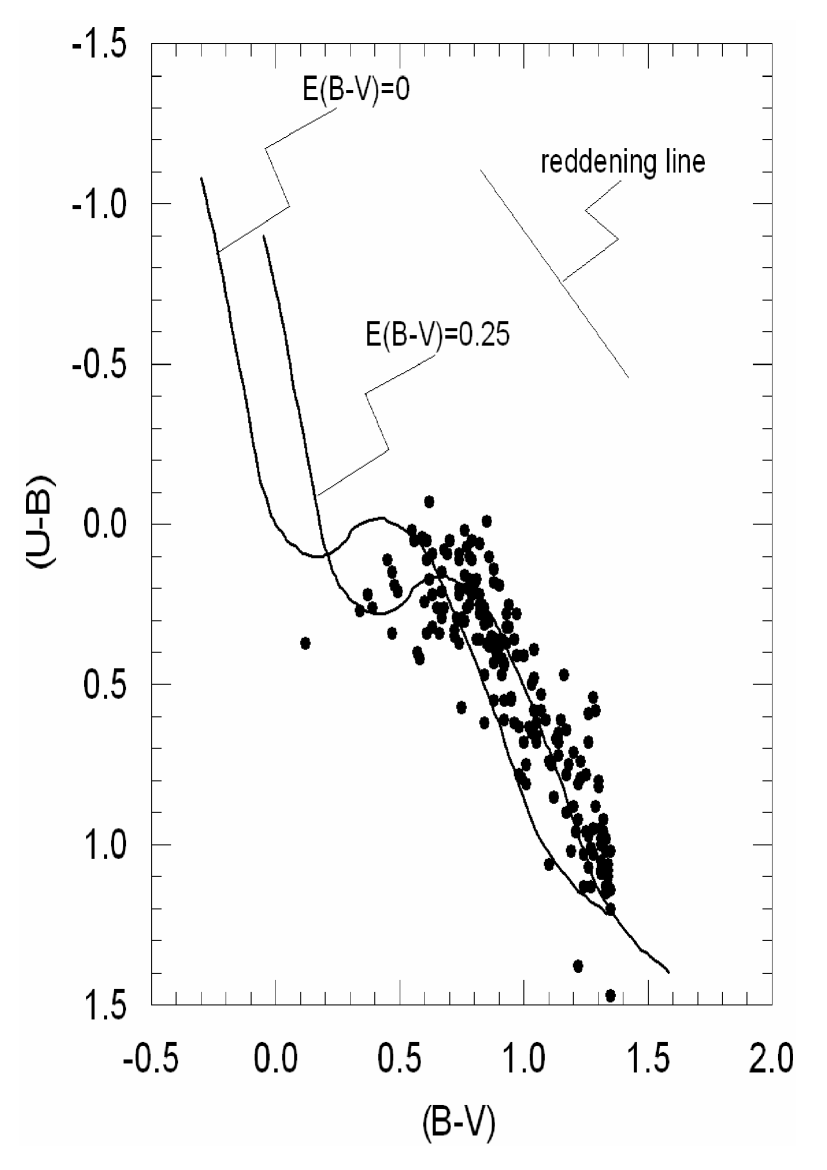
Figure 1: Two-colour diagram for stars used for estimation of the colour-excess, $E(B-V)=0.25$ mag.

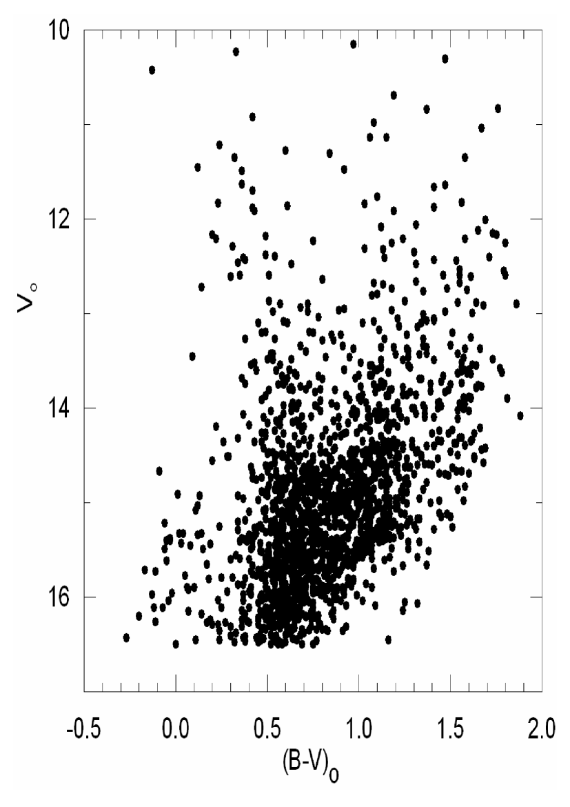
Figure 2: De-reddened colour magnitude diagram for the field SA 133.

2.2 Separation of dwarfs and evolved stars

The $V$-fractioned two-colour diagrams in Fig. 3 show that there is a considerable amount of metal-rich stars consistent with the direction of our field. The positions of some stars in our two-colour diagrams seem to be affected by the scattering which is unavoidable in the photographic photometry for faint stars. The most conspicuous appearance of these stars are those occupying the position of the most metal-rich stars though they are not so large in number to affect our results. Contrary to the metal-rich stars, extreme metal-poor stars ($[Fe/H]<-3.0$ dex) are sparse, especially in apparently bright $V-$ intervals. Such stars exist in all two-colour diagrams in the $UBV$ and $RGU$ systems and sometimes they are in an unexpected considerable amount of number (Karataş et al. 2001). Hence, they are excluded from statistics without regarding their identity which can be binary stars, extra-galactic objects or their position may be affected by relatively large photographic errors which is the case for faint magnitudes. The iso-metallicity lines, for the range $-3\leq[Fe/H]\leq+1$ dex, in Fig. 3 were adopted from Lejeune, Cuisinier, & Buser (1997).

The separation of dwarfs and evolved stars (sub-giants or giants) was carried out to obtain a luminosity function consistent with the local luminosity function of nearby stars due to Gliese & Jahreiss (1992) and Jahreiss & Wielen (1997). The procedure of this separation is based on the fact that the local luminosity functions obtained for many fields indicated a systematic excess of star counts relative to the luminosity function of nearby stars for the fainter segment, i.e. $M(G)\geq 6$ mag, and a deficit for the brighter segment, $M(G)<5$ mag. The excess cited is due to the contamination of evolved stars and it is difficult to separate them from the dwarfs due to the lack of a spectral band sensitive to the surface gravity, $log~{}g$, in the $UBV$ and $RGU$ photometric systems. However, it was shown in some recent works, if apparently bright stars with $M(G)\geq 6$ mag on the main sequence are removed to the category of evolved stars, both segments cited above converge to the local luminosity function of nearby stars (Karaali 1992; Ak et al. 1998; Karataş et al. 2001; Karaali et al. 2004). Because this process causes decrease in the number of absolutely faint stars, $M(G)\geq 6$ mag, whereas it increases the number of bright stars. The apparent limiting magnitude of bright stars considered, lies within $15<G<16$ mag. The best fit between the local luminosity function deduced in this work and the local luminosity function of nearby stars resulted, from iterations, when stars apparently brighter than $V_{o}=15.5$ mag and absolutely fainter than $M(V)=5.5$ mag on the main sequence were assumed to be evolved stars. Thus, brighter absolute magnitudes were attributed to them and they were separated to giant - or sub-giant - category according to their magnitudes, i.e. $M(V)\leq 2$ mag and $M(V)>2$ mag, respectively.

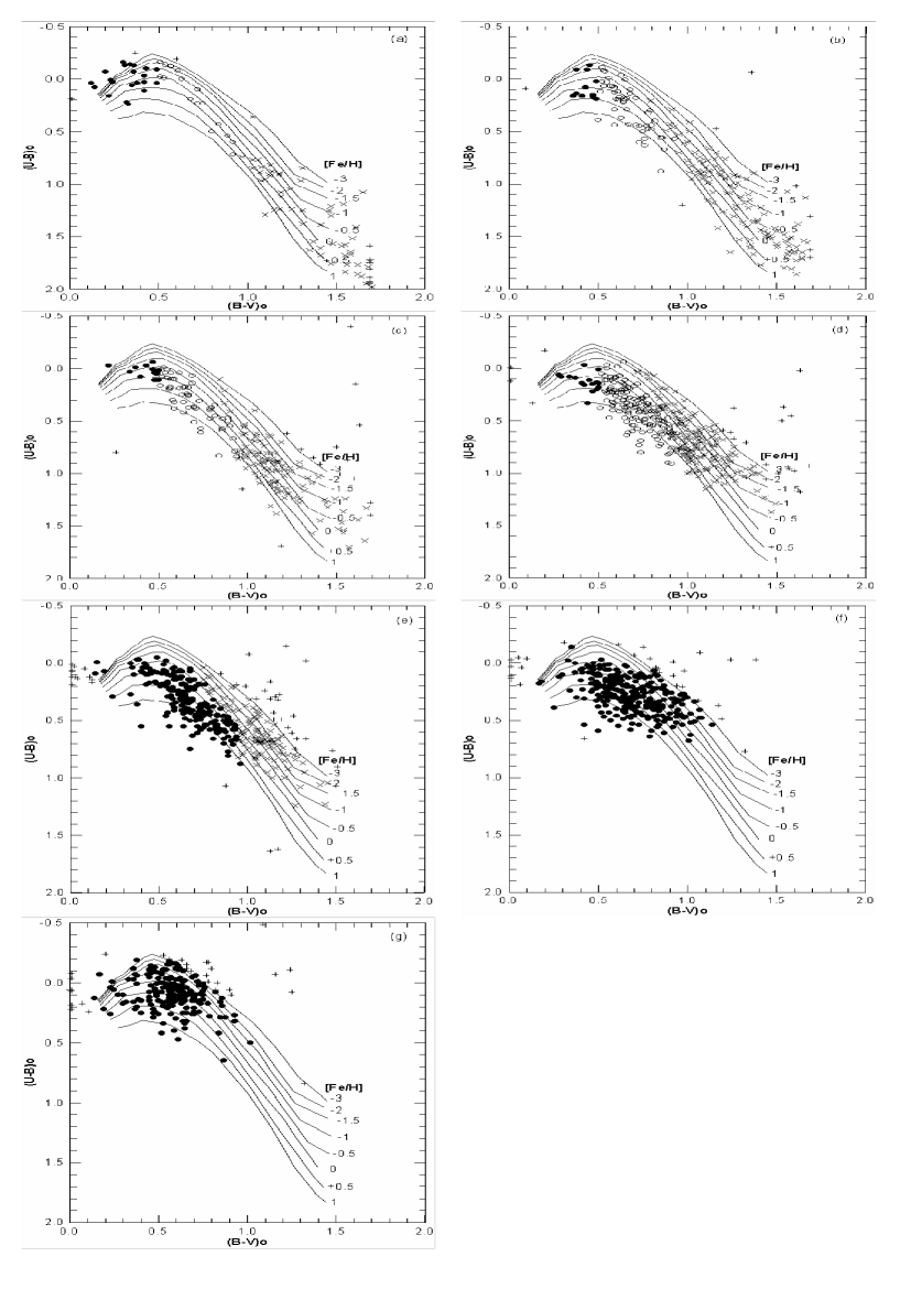
Figure 3: The $V$-fractioned two-colour diagrams: (a) $V_{0}\leq 13.0$, (b) (13.0 14.0], (c) (14.0 14.5], (d) (14.5 15.0], (e) (15.0 15.5], (f) (15.5 16.0], and (g) (16.0 16.5]. Symbols: ($\bullet$): dwarfs, (o): sub-giants, (x): giants, and $(+)$: not included into statistics due to its position in the two-colour diagram. The iso-metallicity lines, $-3\leq[Fe/H]\leq+1$ dex, were adopted from the synthetic data of Lejuene et al. (1997).

2.3 Absolute magnitude and metallicity determination

The absolute magnitudes and metallicities are evaluated by means of two methods. For dwarfs with $[Fe/H]\geq-1.75$ dex, we adopted the metallicity-luminosity calibration of Laird, Carney, & Latham (LCL 1988) which is given in terms of the offset in absolute $V$ magnitude from the Hyades main sequence, for which they obtained

$$M(V)_{(Hyades)}=5.64(B-V)+1.11$$ (1)

The metallicity-dependent offset from this fiducial sequence that LCL derived ($\Delta{M^{H}_{V}}$) is, for a star of given $(B-V)$ colour and given UV-excess $\delta$;

$${}^{\Delta{M^{H}_{V}}=[\frac{2.31-1.04{(B-V)_{o}}}{1.594}][-0.6888\delta+53.14\delta^{2}-97.004\delta^{3}]}$$ (2)

LCL state this calibration to be valid for $\delta~{}\leq 0.25$, which corresponds to $[Fe/H]\geq-1.75$ dex with Carney (1979) transformation of $\delta$ into $[Fe/H]$, as used by LCL and recently by Gilmore et al. (1995).

$$[Fe/H]=0.11-2.90\delta-18.68~{}\delta^{2}$$ (3)

As already cited, the calibration of LCL is valid only for dwarfs with $[Fe/H]\geq-1.75$ dex. Hence another method was necessary for additional metal-poor dwarfs and evolved stars of any metallicity, for absolute magnitude and metallicity derivation. With a optimistic approach, the $(U-B,B-V)$ two-colour diagram calibrated for iso-metallicity lines ($-3\leq[Fe/H]\leq+1$ dex) for dwarfs and evolved stars individually, by means of the synthetic data of Lejeune et al. (1997), can provide metallicities with appropriate interpolation. For absolute magnitude derivation of giant stars, we calibrate $M(V)-(B-V)_{0}$ relation, using published data from of various Galactic globular clusters to cover a large range of metal abundances. The globular clusters used are M92 ($[Fe/H]=-2.24$ dex), M5 (-1.40), 47 Tuc. (-0.71), and M67 (0.00), respectively, (Stetson & Harris 1988; Richer & Fahlman 1987; Hesser et al. 1987; Montgomery, Marschall, & Janes 1993).

For the metallicity calibration of Carney (1979), an error of $\pm$ 0.02 mag in $\delta$ yields an uncertainty of 0.3 dex. The accuracy of the calibration of the Basel Library Spectra (Lejeune et al. 1997) is in level of less than 0.05 mag, implying an uncertainty in derived $[Fe/H]$ of up to 0.35 dex. The uncertainties in derived metallicities from two method are approximately the same. We assumed that the same holds for late-type giants. The uncertainty $\pm$ 0.03 mag in $(B-V)_{o}$, cited above, corresponds to $\pm$ 0.2 mag in absolute magnitude $M(V)$ derived by the colour-magnitude diagrams of four clusters. Combination of the uncertainities in $V_{o}$ and $M(V)$ in the equation gives the distance $r$ to the star, i.e.

$$V_{o}-M(V)=5log(r)-5$$ (4)

amounts to an uncertainty of 10$\%$, in the distance estimate, which is less than the one (20$\%$) cited by Gilmore et al. (1995).

Table 1: The logarithmic space densities $D^{*}$ for dwarfs and sub-giants for all population types (distances in $kpc$, volumes in $pc^{3}$. The symbols are defined in the text. Underlines indicate limiting distance of completeness.

M(V)		$\rightarrow$	(2 3]		(3 4]		(4 5]		(5 6]		(6 7]		(7 8]
$r_{1}$ - $r_{2}$	$\Delta V_{1,2}$	$\bar{r}$	N	D*	N	D*	N	D*	N	D*	N	D*	N	D*
0.00 - 0.40	1.22 (03)	0.32											2	7.22
0.00 - 0.63	4.85 (03)	0.50									24	7.69
0.00 - 1.00	1.93 (04)	0.79	8	6.62	35	7.26			55	7.45
0.00 - 1.58	7.68 (04)	1.26					83	7.03
0.40 - 0.63	3.63 (03)	0.54											30	7.92
0.63 - 1.00	1.44 (04)	0.86									60	7.62
1.00 - 1.58	5.75 (04)	1.36	15	6.42	46	6.90			74	7.11	7	6.09
1.58 - 2.51	2.29 (05)	2.15	52	6.36	176	6.89	114	6.70	9	5.59
2.51 - 3.98	9.12 (05)	3.41	39	5.63	76	5.92	10	5.04
3.98 - 6.31	3.63 (06)	5.40	40	5.04	4	4.04
6.31 - 10.00	1.44 (07)	8.55	3	3.32
		$s(\pm)$		0.27		0.13		0.13		0.17		0.00		0.53

3 Density and luminosity functions

Logarithmic space densities, $D^{*}=logD+10$ are evaluated for dwarfs and sub-giants for consecutive absolute magnitude intervals, i.e. (2 3], (3 4], (4 5], (5 6], (6 7], and (7 8] (Table 1), and for late-type giants (Table 2), where $D(r)=N/\Delta V_{1,2}$, N: number of stars in the partial volume $\Delta V_{1,2}=(\pi/180)^{2}(\sq/3)(r_{2}^{3}-r_{1}^{3})$, $r_{1}$, $r_{2}$: limiting distances of $\Delta V_{1,2}$, $\sq$: 0.19 square-degree, apparent size of the field, $\bar{r}=[(r^{3}_{1}+r^{3}_{2})/2]^{1/3}$ centroid distance of the corresponding partial volume $\Delta V_{1,2}$.

Table 2: The logarithmic space densities for late-type giants (symbols as in Table 1). The standard deviation is $s$ = $\pm$0.39.

$r_{1}-r_{2}$	$\Delta V_{1,2}$	$\bar{r}$	N    D*
0.00-3.98	1.22 (6)	3.16	111    5.96
3.98-6.31	3.63 (6)	5.40	112    5.49
6.31-10.0	1.44 (7)	8.55	122    4.93
10.00-15.85	5.75 (7)	13.55	108    4.27
15.85-25.12	2.29 (8)	21.48	58     3.40
25.12-39.81	9.12 (8)	34.05	40     2.64

The density functions are compared with the galactic model of Gilmore & Wyse (GW, 1985), and Buser et al. (BRK, 1998; 1999) given in the form $\Delta logD(r)=logD(r,l,b)-logD(0,l,b)$ versus $r$, where $\Delta logD(r)$ is the logarithmic difference of the densities at distances $r$ and at the Sun. Thus $\Delta logD(r)=0$ points the logarithmic space density at $r=0$ which is available for luminosity function determination. The comparison is carried out as explained in several studies of the Basel fields (Del Rio & Fenkart 1987; Fenkart & Karaali 1987), i.e. by shifting the model curve perpendicular to the distance axis until the best fit to the histogram results at the centroid distances (Fig. 4a-g). Both models involve two disk components, thin and thick disk, and the de Vaucauleurs spheroid. The parameters for two models are given in Table 3. Although the two set of parameters (especially the scale heights) are different from each other, the model gradients (solid line for the model GW and dashed line for the model BRK) are close to each other in Fig. 4a-f, probably due to relatively short distances ($r<4$ kpc). Actually, the last histogram section for giants (Fig. 4g), $25.12<r\leq 39.81$ kpc, show that the model gradient for BRK begins to diverge from the model gradient for GW at larger distances. There is adequate agreement between GW and BRK models and the observed density functions for dwarfs and sub-giants within the limiting distances of completeness marked by horizontal thick lines in Table 1 and the same agreement results, when one includes the local luminosity function. The luminosity function close to the Sun: $\varphi^{*}(M)$, i.e. the logarithmic space density for the stars with $M$ $\pm~{}0^{m}.5$ at $r$ = 0 is the $D^{*}$ -value corresponding to the intersection of the model-curve with the ordinate axis of the histogram concerned. Fig. 5 shows the agreement between the luminosity function resulting from comparison of our space density data with the GW model and the local luminosity functions of GJ and JW.

Table 3: Parameters for the models of GW and BRK. The symbols give: $n_{i}$: local space density, $H_{i}$: scale-height, $h_{i}$: scale-length, $c/a$: axis ratio for the halo (scale heights and scale lengths in pc).

Population	Parameter	GW	BRK
thin disk	$n_{1}$	1	1
	$H_{1}$	300	290
	$h_{1}$	4000	4010
thick disk	$n_{2}/n_{1}$	0.02	0.06
	$H_{2}$	1000	910
	$h_{2}$	4000	4250
halo	$n_{3}/n_{1}$	0.001	0.0005
	$c/a$	0.85	0.84

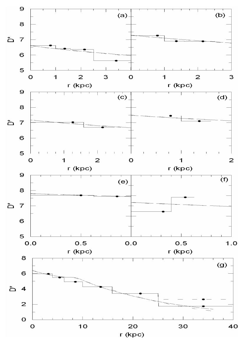
Figure 4: Logarithmic space density functions for dwarfs and sub-giants for six consecutive absolute magnitude intervals: (a) (2 3], (b) (3 4], (c) (4 5], (d) (5 6], (e) (6 7], (f) (7 8]; and for late-type giants (g). Thin solid and dashed lines represent model gradient of GW and BRK, respectively. The last histogram section ($25.12<r\leq 39.81$ kpc) with dashed line corresponds to the density for stars in excess.

However there is some difference between GW model and the observed density function for late type giants (Fig. 4g), extending up to $r\approx 40$ kpc ($z\approx 7$ kpc distance to the Galactic plane). Actually there are 35 stars in excess in the last distance interval which cannot be adopted as dwarfs due to the agreement of the luminosity function with the ones cited above. It is interesting that the same stars do show an excess in the comparision between BRK model and the observed density function. Although the gradients for two models do not fit in every distance interval, i.e. the gradient for the model of BRK is slight above the model gradient of GW at $r\approx 16$ kpc and it is below for the distance interval $r\geq 26$ kpc, they present the same local space density. We do not have enough information for the exact identification of these stars in excess. They may be related to the fact that a number of stars have been eliminated because they have been assigned a too faint metallicity ($[Fe/H]<-3$ dex) or they may be extra-galactic objects. If the stars mentioned in the first case were not eliminated the observed densities in the preceding distance intervals would be increased and there would not be appeared stars in excess in the last distance interval. In this case the local space density would be closer the the one of Gliese (1969). The second case seems also a solution for the problematic 35 stars, because the number of extra-galactic objects increases when one goes to faint magnitudes. Unfortunately the identification of the extra-galactic objects in this field could not be carried out by the University of Minnesota due to its low Galactic latitude ($b=+10^{\circ}.3$). If we omit these stars in excess, we obtain a logarithmic local space density $D^{*}(0)=6.40$ between those of Gliese (1969) and Fenkart (1989c), i.e. $\odot=6.64$ and $D^{*}(0)=6.29$, respectively. The errors for the density functions are given in Tables 1 and 2, and in Fig. 5 in standard deviations.

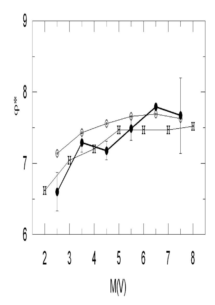
Figure 5: Luminosity function for SA 133 resulting from comparison of observed histograms with the model gradient GW ($\bullet$), and confronted to the luminosity functions of GJ ($\odot$), and JW (H).

4 Metallicity distribution

A gaussian fit to the metallicity distribution for dwarfs and sub-giants (Fig. 6a) shows a high and narrow peak at $[Fe/H]=+0.13$ dex and a long metal-poor tail, though with less contribution to the total metallicity, expected for a low-latitude field to the galactic centre direction. Contrary to dwarfs and sub-giants, metallicity distribution for late-type giants which extend up to $r=25$ kpc relative to the Sun or $z=4.5$ kpc above the galactic plane thus forming a sub-sample of different population types is multi-modal (Fig. 6b). A gaussian fit to Fig. 6b gives two peaks at $[Fe/H]=+0.12$, $-0.83$ dex, and additionally a flat metal-poor tail extending down to $[Fe/H]=-3$ dex.

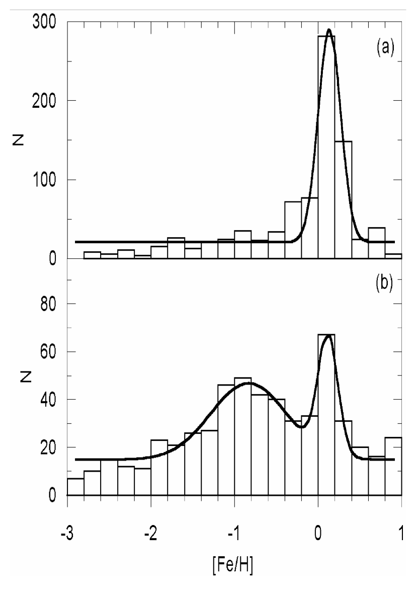
Figure 6: Metallicity distribution for dwarfs and sub-giants (a), and late-type giants (b). Curves in (a) and (b) are the fitted gaussian distributions.

Each histogram in Fig 7a-c is fitted a gaussian curve with a mean $<[Fe/H]>=-0.14$, $-0.78$, and $-1.10$ dex. $z$-heights shown in the panels are $<z>=0.96$, $1.72$, and $2.20$ kpc, respectively. One can notice that a systematic shift from metal rich stars to the metal poor ones in Fig. 7a-c, where the mean metallicity as a function of $z$ distance is displayed.

Comparison of the mean metal abundances and $<z>$ distances with any of these panels gives metallicity gradients as follows
$d[Fe/H]/dz=[(-0.78)-(-0.14)]/(1.72-0.96)=-0.84$ dex kpc^-1
$d[Fe/H]/dz=[(-1.10)-(-0.14)]/(2.20-0.96)=-0.77$ dex kpc^-1
$d[Fe/H]/dz=[(-1.10)-(-0.78)]/(2.20-1.72)=-0.67$ dex kpc^-1

The gaussian of Fig. 7d shows a peak at $<[Fe/H]>=-1.35$ dex, with a $<z>=3$ kpc, which reveal three metallicity gradients close to each other but different than cited above, when compared with the data in each former panels. The mean of these metallicity gradients, i.e. $d[Fe/H]/dz=-0.45$ dex kpc^-1, give the indication that metallicity gradient is less steep in the outward of the Galaxy.

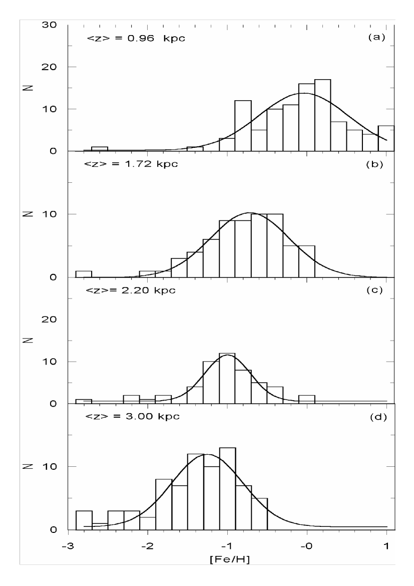
Figure 7: Metallicity distributions for late-type giants for four $z$-intervals which reveal a metallicity gradient into the direction of the Galactic centre. Curves in each panel are the fitted gaussian distributions.

The mean $z$-distance 1 kpc corresponding to a mean distance 5.7 kpc in the Galactic plane lies in the dominant region of thin disk, and the corresponding metallicity gradient, $d[Fe/H]/dz$ = -0.84 dex kpc^-1, is close to the one given by Trefzger, Pel, & Gabi (1995) ($d[Fe/H]/dz$ = -0.55 $\pm$ 0.10 dex kpc^-1) up to $z$ = 0.9 kpc for a field investigated by means of Walraven $VBLUW$ photometry. These authors claim a less steep gradient, -0.23 $\pm$ 0.04 dex kpc^-1, for $z<4$ kpc, however. The metallicity gradient for thin disk, deduced from the investigation of seven fields by Rong et al. (2001), very recently, is $d[Fe/H]/dz>-0.6$ dex kpc^-1, not contradicting with our results, within the limits of accuracy. Stars in the third and fourth panels ($<z>$ = 2.2 and 3 kpc) in our work sample the galactic halo for which metallicity gradient is not controversial. Thus, the metallicity gradient for stars in the second panel ($<z>$ = 1.72 kpc) to be discussed, for the region occupied by these stars is dominant by thick disk. Such a metallicity gradient contradicts some formation histories postulated for the formation of the (classical) thick disk. Until recent years this component of our Galaxy was assumed to have a mean metal abundance $[Fe/H]\sim-0.60$ dex, a scale-height $H\leq 1$ kpc, and its space number density 2 - 8 % of the thin disk in the solar neighbourhood. Additionally, and more important, it was argued that the stars of thick disk were formed from a merger into the Galaxy (cf. Norris 1996 and references within), a formation mechanism unlikely to leave an abundance gradient. Some recent works suggested that the thick disk is more important component of the Galaxy, extending up to $\sim 3-5$ kpc from the galactic plane (Majewski 1993) with a metal-poor (Norris 1996) and a metal-rich tail (Carney 2000; Karaali et al. 2000; Karaali et al. 2004). Hence a revision of the formation scenario of the thick disk may be required. Furthermore, the works of Reid & Majewski (1993) and Chiba & Yoshii (1998) also suggest a metallicity gradient for the thick disk.

5 Conclusion

The agreement of the luminosity function resulting from the comparison of GW model with the logarithmic space density functions for stars with $2<M(V)\leq 8$ mag, and the logarithmic space density function for late-type giants with the same model (and also with the model BRK) confirm the separation of dwarfs and evolved stars in our field.

There is a concentration at $[Fe/H]=+0.13$ dex and a long tail down to $[Fe/H]\sim-3$ dex for the metallicity distribution for dwarfs and sub-giants as expected for a low latitude field into the galactic centre direction with a short apparent limiting magnitude, i.e. $V_{o}$=16.5 mag. Whereas late-type giants which lie up to large distances relative to the Sun or up to large $z$-heights from the galactic plane have multi-modal metallicity distribution. However, the weighted mean metal-abundances of late-type giants in our sample is $<[Fe/H]>=-0.7$ dex, rather close to the one claimed by Morrison & Harding (1993), i.e. $-0.8$ dex, who investigated only the K giants in two square degree field almost symmetric to ours relative to the galactic plane ($l=350^{\circ}$, $b=-10^{\circ}$) and to Harding’s (1996) finding, $<[Fe/H]>=-0.8$ dex, for G and K giants.

In this work, we observed metallicity gradient in each of the populations. This is different than the one usually expected: the metallicity gradient may appear when there is a mixing of populations for which the relative proportion of the populations changes along the line of sight. In such case it results in a gradient which may not be present in each of the populations. However, in the present data there is a variable proportion of the populations when $z$ is increasing, indicating a gradient in the populations. Additionally, it is rather steep in the regions dominated by thin and thick disks, i.e. $d[Fe/H]/dz=-0.75$ dex kpc^-1. As cited in Section 4, Reid & Majewski (1993) and Chiba & Yoshii (1998) also suggest a metallicity gradient for the thick disk. All these works would have implications on the discussion about the scenario of formation of the thick disk. However, we recognize that there are significant statistical uncertainties in our resuls, due to photographic data. It is also probable that the direction of our field ($l=6^{\circ}.5$) may play a specific role on our results.

- [1] Ak, S. G., Karaali, S., & Buser, R.: 1998, A&AS, 131, 345
- [2] Bahcall, J. N.: 1986, ARA&A, 24, 577
- [3] Becker, W.: 1965, ZA, 62, 54
- [4] Becker, W., & Svopoulos, S.: 1976, A&AS, 23, 97
- [5] Becker, W., & Fang, C.: 1982, A&A, 49, 61
- [6] Becker, W., & Hassan, S.M.: 1982, A&A, 47, 247
- [7] Becker, W., Morales-Duran, C., Ebner, E., Esin-Yilmaz, F., Fenkart, R., Hartl, H., & Spaenhauer, A.: 1982. Photometric Catalogue for Stars in Selected Areas and other Fields in the - Systems (VIII)
- [8] Burnstein, D., & Heiles, C.: 1982, AJ, 87, 1165
- [9] Buser, R., Rong, J., & Karaali, S.: 1998, A&A, 331, 934 (BRK)
- [10] Buser, R., Rong, J., & Karaali, S.: 1999, A&A, 348, 98
- [11] Carney, B. W.: 1979, ApJ, 233, 211
- [12] Carney, B. W.: 2000, The Galactic Halo: from Globular Clusters to Field Stars. Liége Intr. Astr. Coll. Edts. A. Noel et al., p. 287
- [13] Chen, B., Stoughton, C., Smith, J. A., Uomoto, A., Pier, J. R., Yanny, B., Ivezic, Z., York, D. G., Anderson, J. E., Annis, J., Brinkmann, J., Csabai, I. Fukugita, M., Hindsley, R., Lupton, R., Munn, J. A., and the SDSS Collaboration: 2001, ApJ, 553, 184
- [14] Chiba, M., & Yoshii, Y.: 1998, AJ, 115, 168
- [15] Del Rio, G., & Fenkart, R. P.: 1987, A&AS 68, 397
- [16] Fenkart, R. P., Topaktaş, L., Boydag, S., & Kandemir, G.: 1986, A&AS, 63, 49
- [17] Fenkart, R. P., & Karaali, S.: 1987, A&AS, 69, 33
- [18] Fenkart, R. P.: 1989a, A&AS, 78, 217
- [19] Fenkart, R. P.: 1989b, A&AS, 79, 51
- [20] Fenkart, R. P.: 1989c, A&AS, 80, 89
- [21] Fenkart, R. P.: 1989d, A&AS, 81, 187
- [22] Fenkart, R. P., & Karaali, S.: 1990, A&AS, 83, 481
- [23] Gilmore, G., & Reid, N.: 1983, MNRAS, 202, 1025
- [24] Gilmore, G., & Wyse, R. F. G.: 1985, AJ, 90, 2015 (GW)
- [25] Gilmore, G., Wyse, R. F. G., & Jones, J. B.: 1995, AJ, 109, 1095
- [26] Gliese, W.: 1969, Veröff. Astron. Rechen-Inst. Heidelberg, No:22
- [27] Gliese, W., & Jahreiss, H.: 1992, Nearby Stars Preliminary 3 rd. version Astron. Rechen-Inst. Heidelberg (GJ)
- [28] Harding, P.: 1996, in Formation of the Galactic Halo, ed. H. Morrison, & A. Sarajedeni (San Fransisco, ASP), Vol.92, p.152.
- [29] Hersperger, T.: 1973, A&A, 22, 195
- [30] Hesser, J. W., Harris, W. E., Vandenberg, D. A., Allwright, J. W. B., Shott, P., & Stetson, P. B.: 1987, PASP, 99, 739
- [31] Jahreiss, H., & Wielen, R.: 1997, ESASP 402, 675, eds. Battrick, B., Perryman, M. A. C., & Bernacca, P. L. (JW)
- [32] Karaali, S.: 1992, VIII. Nat. Astron. Symp. Eds. Z. Aslan and O. Gölbaşı, Ankara - Turkey, p.202
- [33] Karaali, S., Karataş, Y., Bilir, S., Ak, S. G., & Gilmore, G. F.: 2000, The Galactic Halo: from Globular Clusters to Field Stars. Liége Intr. Astr. Coll. Edts. A. Noel et al., p. 353
- [34] Karaali, S., Ak, S. G., Bilir, S., Karataş, Y., & Gilmore, G.: 2003, MNRAS, 343, 1013
- [35] Karaali, S., Bilir, S., & Buser, R.: 2004, PASA (accepted)
- [36] Karataş, Y., Karaali, S., & Buser, R.: 2001, A&A, 373, 895
- [37] Laird, J. B., Carney, B. W., & Latham, D. W.: 1988, AJ, 95, 1843 (LCL)
- [38] Lejeune, Th., Cuisinier, F., & Buser, R.: 1997, A&AS, 125, 229
- [39] Majewski, S. R.: 1993, ARA&A, 31, 575
- [40] Mermilliod, J. C., & Mermilliod, M.: 1994 Catalogue of Mean UBV Data on Stars, VI, 1387 p, Springer-Verlag Berlin Heidelberg New York
- [41] Montgomery, K. A., Marschall, L. A., & Janes, K. A.: 1993, AJ, 106, 181
- [42] Morrison, H. L., & Harding, P.: 1993, PASP, 105, 977
- [43] Norris, J. E.: 1996, ASP Conf. Ser. Vol. 92, p.14, Eds. H. L. Morrison & A. Sarajedini
- [44] Reid, N., & Majewski, S. R.: 1993, ApJ, 409, 635
- [45] Richer, H. B., & Fahlman, G. G.: 1987, ApJ, 316, 189
- [46] Robin, A. C., Reylé, C., & Crézé, M.: 2000, A&A, 359, 103
- [47] Robin, A. C., Reylé, C., Derriére, S., & Picaud, S.: 2003, A&A, 409, 523
- [48] Rong, J., Buser, R., & Karaali, S.: 2001, A&A, 365, 431
- [49] Sandage, A.: 1969, ApJ, 158, 1115
- [50] Schlegel, D. J., Finkbeiner, D. P., & Davis, M.: 1998, ApJ, 500, 525
- [51] Siegel, M. H., Majewski, S. R., Reid, I. N., & Thompson, I. B.: 2002, ApJ, 578, 151
- [52] Stetson, P. B., & Harris, W. E.: 1988, AJ, 96, 909
- [53] Trefzger, Ch., Pel, J. W., & Gabi, S.: 1995, A&A, 304, 381