The Physics of Gamma-Ray Bursts

Abstract

Gamma-Ray Bursts (GRBs), short and intense pulses of low energy $\gamma$-rays , have fascinated astronomers and astrophysicists since their unexpected discovery in the late sixties. During the last decade, several space missions: BATSE (Burst and Transient Source Experiment) on Compton Gamma-Ray Observatory, BeppoSAX and now HETE II (High-Energy Transient Explorer), together with ground optical, infrared and radio observatories have revolutionized our understanding of GRBs showing that they are cosmological, that they are accompanied by long lasting afterglows and that they are associated with core collapse Supernovae. At the same time a theoretical understanding has emerged in the form of the fireball internal-external shocks model. According to this model GRBs are produced when the kinetic energy of an ultra-relativistic flow is dissipated in internal collisions. The afterglow arises when the flow is slowed down by shocks with the surrounding circum-burst matter. This model has numerous successful predictions like the prediction of the afterglow itself, the prediction of jet breaks in the afterglow light curve and of an optical flash that accompanies the GRBs themselves. In this review I focus on theoretical aspects and on physical processes believed to take place in GRBs.

I INTRODUCTION

Gamma-Ray Bursts (GRBs) are short and intense pulses of soft $\gamma$-rays . The bursts last from a fraction of a second to several hundred seconds. GRBs arrive from cosmological distances from random directions in the sky. The overall observed fluences range from $10^{-4}$ergs/cm² to $10^{-7}$ergs/cm² (the lower limit depends, of course, on the characteristic of the detectors and not on the bursts themselves). This corresponds to isotropic luminosity of $10^{51}-10^{52}$ergs/sec, making GRBs the most luminous objects in the sky. However, we know today that most GRBs are narrowly beamed and the corresponding energies are “only” around $10^{51}$ergs Frail et al. (2001); Panaitescu and Kumar (2001); Piran et al. (2001), making them comparable to Supernovae in the total energy release.

The GRBs are followed by afterglow - lower energy, long lasting emission in the X-ray, optical and radio. The radio afterglow was observed in some cases several years after the bursts. The accurate afterglow positions enabled the identification of host galaxies in almost all cases when afterglow was detected and this in turn enabled the determination of the corresponding redshifts that range from 0.16 (or possibly even down to 0.0085) to 4.5. Within the host galaxies there is evidence that (long duration) GRBs arise within star forming regions and there is evidence that they follow the star formation rate.

While not all observed features are understood there is an overall agreement between the observations and the fireball model. According to the fireball model GRBs are produced when the kinetic energy of an ultra-relativistic flow is dissipated. The GRB itself is produced by internal dissipation within the flow while the afterglow is produced via external shocks with the circum-burst medium. I will focus in this review on this model.

The numerous observations of the GRB and the observations of the afterglow constrain the fireball model that describes the emitting regions. The evidence on nature of the inner engine that powers the GRB and produces the ultra-relativistic flow is however, indirect. The energetic requirements and the time scales suggest that GRB involve the formation of the black hole via a catastrophic stellar collapse event or possibly a neutron star merger. Additional indirect evidence arises from the requirement of the fireball model of long (several dozen seconds) activity of the inner engine. This hints towards an inner engine built on an accreting black hole. On the other hand, the evidence of association of GRBs with star forming regions indicates that GRBs progenitors are massive stars. Finally, the appearance of Supernova bumps in the afterglow light curve (most notably in GRB 030329) suggest association with Supernovae and stellar collapse.

I review here the theory of GRB, focusing as mentioned earlier on the fireball internal-external shocks model. I begin in §II with a brief discussion of the observations. I turn in §III to some generally accepted properties of GRB models - such as the essential ultra-relativistic nature of this phenomenon. Before turning to a specific discussion of the fireball model I review in §IV several relativistic effects and in §V the physical process, such as synchrotron emission or particle acceleration in relativistic shocks that are essential ingredients of this model. In §VI I turn to a discussion of the prompt emission and the GRB. In §VII I discuss modelling the afterglow emission. I consider other related phenomenon - such as TeV $\gamma$-rays emission, high energy neutrinos, Ultra High energy cosmic rays and gravitational radiation in §VIII. Finally, I turn in §IX to examine different ‘inner engines’ and various aspects related to their activity. I conclude with a discussion of open questions and observational prospects.

While writing this review I realized how large is the scope of this field and how difficult it is to cover all aspects of this interesting phenomenon. Some important aspects had to be left out. I also did not attempt to give a complete historical coverage of the field. I am sure that inadvertently I have missed many important references. I refer the reader to several other recent review papers Fishman and Meegan (1995); Piran (1999); van Paradijs et al. (2000); Piran (2000); Mészáros (2001); Hurley et al. (2002e); Mészáros (2002); Galama and Sari (2002) that discuss these and other aspects of GRB theory and observations from different points of view.

II OBSERVATIONS

I begin with a short review of the basic observed properties of GRBs. This review is brief as a complete review requires a whole paper by itself. I refer the reader to several review papers for a detailed summary of the observations Fishman and Meegan (1995); van Paradijs et al. (2000); Hurley et al. (2002e); Galama and Sari (2002). I divide this section to three parts. I begin with the prompt emission - the GRB itself. I continue with properties of the afterglow. I conclude with a discussion of the rates of GRBs, the location of the bursts within their host galaxies and the properties of the host galaxies.

II.1 Prompt Emission

I begin with a discussion of the GRB itself, namely the $\gamma$-rays and any lower-energy emission that occurs simultaneously with them. This includes X-ray emission that generally accompanies the $\gamma$-ray emission as a low energy tail. In some cases, called X-ray flashes (XRFs), the $\gamma$-rays signal is weak and all that we have is this X-ray signal. Prompt (operationally defined as the time period when the $\gamma$-ray detector detects a signal above background) longer-wavelength emission may also occur at the optical and radio but it is harder to detect. However, so far optical flashes was observed In three cases Akerlof et al. (1999); Fox et al. (2003b); Li et al. (2003) simultaneously with the $\gamma$-ray emission.

II.1.1 Spectrum

The spectrum is non thermal. The energy flux peaks at a few hundred keV and in many bursts there is a long high energy tail extending in cases up to GeV. The spectrum varies strongly from one burst to another. An excellent phenomenological fit for the spectrum was introduced by Band et al. (1993) using two power laws joined smoothly at a break energy $(\tilde{\alpha}-\tilde{\beta})E_{0}$:

$$N(\nu)=N_{0}\cases{\big{(}{h\nu})^{\tilde{\alpha}}\exp(-{h\nu\over E_{0}})&for $h\nu<(\tilde{\alpha}-\tilde{\beta})E_{0}$ ;\cr\big{[}{(\tilde{\alpha}-\tilde{\beta})E_{0}}\big{]}^{(\tilde{\alpha}-\tilde{\beta})}\big{(}{h\nu}\big{)}^{\tilde{\beta}}\exp(\tilde{\beta}-\tilde{\alpha}),&for $h\nu>(\tilde{\alpha}-\tilde{\beta})E_{0},$\cr}\ .$$ (1)

I denote the spectral indices here as $\tilde{\alpha}$ and $\tilde{\beta}$ to distinguish them from the afterglow parameters ($\alpha$ and $\beta$) discussed later. There is no particular theoretical model that predicts this spectral shape. Still, this function provides an excellent fit to most of the observed spectra. For most observed values of $\tilde{\alpha}$ and $\tilde{\beta}$, $\nu F_{\nu}\propto\nu^{2}N(\nu)$ peaks at $E_{p}=(\tilde{\alpha}+2)E_{0}$. For about 10% of the bursts the upper slope is larger than -2 and there is no peak for $\nu F_{\nu}$ within the observed spectrum. Another group of bursts, NHE bursts, (no high energy) Pendleton et al. (1997) does not have a hard component (which is reflected by a very negative value of $\tilde{\beta}$). The “typical” energy of the observed radiation is $E_{p}$. $E_{p}$ defined in this way should not be confused with the commonly used hardness ratio which is the ratio of photons observed in two BATSE channels: Channel 3 (100-300keV) counts divided by Channel 2 (50-100keV) counts. The break frequency and the peak flux frequencies are lower on average for bursts with lower observed flux Mallozzi et al. (1995, 1998).

Band et al. (1993) present a small catalogue of the spectra of 52 bright bursts which they analyze in terms of the Band function. Preece et al. (2000) present a larger catalogue with 156 bursts selected for either high flux or fluence. They consider several spectral shape including the Band function.

Fig. 1 shows the distribution of observed values of the break energy, $(\tilde{\alpha}-\tilde{\beta})E_{0}$, in a sample of bright bursts Preece et al. (2000). Most of the bursts are the range $100\,{\rm keV}<(\tilde{\alpha}-\tilde{\beta})E_{0}<400\,{\rm keV}$, with a clear maximum in the distribution around $(\tilde{\alpha}-\tilde{\beta})E_{0}\sim 250$keV. There are not many soft GRBs - that is, GRBs with peak energy in the tens of keV range. However, the discovery Heise et al. (2001) of XRFs - X-ray flashes with similar temporal structure to GRBs but lower typical energies - shows that the low peak energy cutoff is not real and it reflects the lower sensitivity of BATSE in this range Kippen et al. (2002).

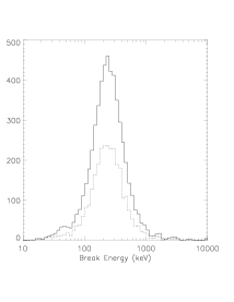
Figure 1: Distribution of the observed values of the break energy $(\tilde{\alpha}-\tilde{\beta})E_{0}$ in a sample of bright bursts Preece et al. (2000)

. The solid line represents the whole sample while the dashed line represent a subset of the data.

Similarly, it is debatable whether there is a real paucity in hard GRBs and there is an upper cutoff to the GRB hardness or it just happens that the detection is optimal in this (a few hundred keV) band. BATSE triggers, for example, are based mostly on the count rate between 50keV and 300keV. BATSE is, therefore, less sensitive to harder bursts that emit most of their energy in the MeV range. Using BATSE’s observation alone one cannot rule out the possibility that there is a population of harder GRBs that emit equal power in total energy which are not observed because of this selection effect Piran and Narayan (1996); Cohen et al. (1997); Lloyd and Petrosian (1999); Higdon and Lingenfelter (1998). More generally, a harder burst with the same energy as a soft one emits fewer photons. Furthermore, the spectrum is generally flat in the high energy range and it decays quickly at low energies. Therefore it is intrinsically more difficult to detect a harder burst. A study of the SMM (Solar Maximum Mission) data Harris and Share (1998) suggests that there is a deficiency (by at least a factor of 5) of GRBs with hardness above 3MeV, relative to GRBs peaking at $\sim$0.5MeV, but this data is consistent with a population of hardness that extends up to 2MeV.

Overall the narrowness of the hardness distribution is very puzzling. First, as I stressed earlier it is not clear whether it is real and not a result of an observational artifact. If it is real then on one hand there is no clear explanation to what is the physical process that controls the narrowness of the distribution (see however Guetta et al. (2001a)). On the other hand cosmological redshift effects must broaden this distribution and it seem likely (but not demonstrated yet) that if the GRB distribution extends to z=10 as some suggest Lamb and Reichart (2000); Ciardi and Loeb (2000); Bromm and Loeb (2002); Lloyd-Ronning et al. (2002) then such a narrow distribution requires an intrinsic correlation between the intrinsic hardness of the burst and its redshift, namely that the intrinsic hardness increases with the redshift. There is some evidence for such a correlation between $E_{p}$ and the observed peak flux Mallozzi et al. (1995, 1998). More recently Amati et al. (2002) reported on a correlation between $E_{p}$ and the isotropic equivalent energy seen in 12 BeppoSAX bursts that they have analyzed. They also report on a correlation between $E_{p}$ and the redshift as, the bursts with higher isotropic equivalent energy are typically more distant. These three different correlations are consistent with each other if the observed peak flux of bursts is determined by their intrinsic luminosity more than by the distance of the bursts. In such a case (because of the larger volume at larger distances) the observed more distant bursts are on average brighter than nearer ones (see also §II.3).

Even though the burst hardness distribution shows a single population a plot of the hardness vs temporal duration shows that short bursts (see Fig. 4) are typically harder Dezalay et al. (1996); Kouveliotou et al. (1996). The correlation is significant. Another interesting sub-group of bursts is the NHE (no high energy) bursts - bursts with no hard component that is no emission above 300keV Pendleton et al. (1997). This group is characterized by a large negative value of $\beta$, the high energy spectral slope. The NHE bursts have luminosities about an order of magnitude lower than regular bursts and they exhibit an effectively homogeneous intensity distribution with $\langle V/V_{max}\rangle=0.53\pm 0.029$. As I discuss later in §II.1.2 most GRB light curves are composed of many individual pulses. It is interesting that in many bursts there are NHE pulses combined with regular pulses.

EGRET (The Energetic Gamma Ray Experiment Telescope) the high energy $\gamma$-rays detector on Compton - GRO detected seven GRBs with photon energies ranging from 100 MeV to 18 GeV Dingus and Catelli (1998). In some cases this very high energy emission is delayed more than an hour after the burst Hurley (1994); Sommer et al. (1994). No high-energy cutoff above a few MeV has been observed in any GRB spectrum. Recently, González et al. (2003) have combined the BATSE (30keV -2Mev) data with the EGRET data for 26 bursts. In one of these bursts, GRB 941017 (according to the common notation GRBs are numbered by the date), they have discovered a high energy tail that extended up to 200 MeV and looked like a different component. This high energy component appeared 10-20 sec after the beginning of the burst and displayed a roughly constant flux with a relatively hard spectral slope ($F_{\nu}\propto\nu^{0}$) up to 200 sec. At late time (150 after the trigger) the very high energy (10-200 MeV) tail contained 50 times more energy than the “main” $\gamma$-rays energy (30keV-2MeV) band. The TeV detector, Milagrito, discovered (at a statistical significance of 1.5e-3 or so, namely at 3$\sigma$) a TeV signal coincident with GRB 970417 Atkins et al. (2000, 2003). If true this would correspond to a TeV fluence that exceeds the low energy $\gamma$-rays fluence. However no further TeV signals were discovered from other 53 bursts observed by Milagrito Atkins et al. (2000) or from several bursts observed by the more sensitive Milagro McEnery (2002). One should recall however, that due to the attenuation of the IR background TeV photons could not be detected from $z>0.1$. Thus even if most GRBs emit TeV photons those photons won’t be detected on Earth.

Another puzzle is the low energy tail. Cohen et al. (1997) analyze several strong bursts and find that their low energy slope is around 1/3 to -1/2. However, Preece et al. (1998, 2002) suggest that about 1/5 of the bursts have a the low energy power spectrum, $\alpha$, steeper than 1/3 (the synchrotron slow cooling low energy slope). A larger fraction is steeper than -1/2 (the fast cooling synchrotron low energy slope). However, this is not seen in any of the HETE spectrum whose low energy resolution is somewhat better. All HETE bursts have a low energy spectrum that is within the range 1/3 and -1/2 Barraud et al. (2003). As both BATSE and HETE use NaI detectors that have a poor low energy resolution Cohen et al. (1997), this problem might be resolved only when a better low energy spectrometer will be flown.

II.1.2 Temporal Structure

The duration of the bursts spans five orders, ranging from less than 0.01sec to more than 100sec. Common measures for the duration are $T_{90}$ ($T_{50}$) which correspond to the time in which 90% (50%) of the counts of the GRB arrives. As I discuss below (see §II.1.3) the bursts are divided to long and short bursts according to their $T_{90}$. Most GRBs are highly variable, showing 100% variations in the flux on a time scale much shorter than the overall duration of the burst. Fig 2 depicts the light curve of a typical variable GRB (GRB 920627). The variability time scale, $\delta t$, is determined by the width of the peaks. $\delta t$ is much shorter (in some cases by a more than a factor of $10^{4}$) than $T$, the duration of the burst. Variability on a time scale of milliseconds has been observed in some long bursts Nakar and Piran (2002c); McBreen et al. (2001). However, only $\sim 80$% of the bursts show substantial substructure in their light curves. The rest are rather smooth, typically with a FRED (Fast Rise Exponential Decay) structure.

Fenimore and Ramirez-Ruiz (2001) (see also Reichart et al. (2001)) discovered a correlation between the variability and the luminosity of the bursts. This correlation (as well as the lag-luminosity relation discussed later) allow us to estimate the luminosity of bursts that do not have a known redshift.

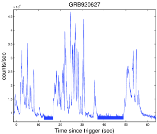
Figure 2: The light curve of GRB 920627. The total duration of the burst is 52sec, while typical pulses are 0.8sec wide. Two quiescent periods lasting $\sim$10 seconds are marked by horizontal solid bold lines.

The bursts seem to be composed of individual pulses, with a pulse being the “building blocks” of the overall light curve. Individual pulses display a hard to soft evolution with the peak energy decreasing exponentially with the photon fluence Liang and Kargatis (1996); Norris et al. (1996); Ford et al. (1995). The pulses have the following temporal and spectral features. (i) The light curve of an individual pulse is a FRED - fast rise exponential decay - with an average rise to decay ratio of 1:3 Norris et al. (1996). (ii) The low energy emission is delayed compared to the high energy emission Norris et al. (1996). Norris et al. (2000) have found that these spectral lags are anti-correlated with the luminosity of the bursts: Luminous bursts have long lags. This lag luminosity relation provides another way to estimate the luminosity of a burst from its (multi-spectra) light curve. (iii) The pulses’ low energy light curves are wider compared to the high energy light curves. The width goes as $\sim E^{-0.4}$Fenimore et al. (1995a). (iv) There is a Width-Symmetry-Intensity correlation. High intensity pulses are (statistically) more symmetric (lower decay to rise ratio) and with shorter spectral lags Norris et al. (1996). (v) There is a Hardness-Intensity correlation. The instantaneous spectral hardness of a pulse is correlated to the instantaneous intensity (the pulse become softer during the pulse decay) Borgonovo and Ryde (2001).

Both the pulse widths, $\delta t$, and the pulse separation,$\Delta t$ , have a rather similar log-normal distributions. However, the pulse separation, distribution, reveals has an excess of long intervals Nakar and Piran (2002c). These long intervals can be classified as quiescent periods Ramirez-Ruiz and Merloni (2001), relatively long periods of several dozen seconds with no activity. When excluding these quiescent periods both distributions are log-normal with a comparable parameters Nakar and Piran (2002c); Quilligan et al. (2002). The average pulse interval, $\bar{\Delta}t=1.3sec$ is larger by a factor 1.3 then the average pulse width $\bar{\delta}t=1sec$. One also finds that the pulse widths are correlated with the preceding interval Nakar and Piran (2002c). Ramirez-Ruiz and Fenimore (2000) found that the pulses’ width does not vary along the bursts.

One can also analyze the temporal behavior using the traditional Fourier transform method to analyze. The power density spectra (PDS) of light curves shows a power law slope of $\sim-5/3$ and a sharp break at 1Hz Beloborodov et al. (2000).

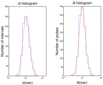
Figure 3: The pulse width distribution (right) and the distribution of intervals between pulses (left) (from Nakar and Piran (2002c)).

The results described so far are for long bursts. the variability of short ($T<2$sec) bursts is more difficult to analyze. The duration of these bursts is closer to the limiting resolution of the detectors. Still most ($\sim 66\%$) short bursts are variable with $\delta t/T<0.1$ Nakar and Piran (2002b). These variable bursts are composed of multiple subpulses.

II.1.3 Populations

Long and Short Bursts The clearest classification of bursts is based on their duration. Kouveliotou et al. (1993) have shown that GRB can be divided to two distinct groups: long burst with $T_{90}>2$sec and short bursts with $T_{90}<2$sec. Note that it was suggested Mukherjee et al. (1998); Horváth (1998) that there is a third intermediate class with $2.5{\rm sec}<T_{90}<7$sec. However, it is not clear if this division to three classes is statistically significant Hakkila et al. (2000).

An interesting question is whether short bursts could arise from single peaks of long bursts in which the rest of the long burst is hidden by noise. Nakar and Piran (2002b) have shown that in practically all long bursts the second highest peak is comparable in height to the first one. Thus, if the highest peak is above the noise so should be the second one. Short bursts are a different entity. This is supported by the observation that short bursts are typically harder Dezalay et al. (1996); Kouveliotou et al. (1996). The duration-hardness distribution (see Fig. 4) shows clearly that there are not soft short bursts.

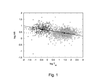
Figure 4: The hardness-duration correlation for BATSE bursts. HR is the ratio of fluence between BATSE channels 3 and 2. Squares represent short burst and circle long bursts. The solid line is a regression line for the whole sample. The two dotted lines are the regresions lines for the short and long samples respectively (from Qin et al. (2000).)

The spatial distribution of the observed short bursts is clearly different from the distribution of the observed long one. A measure of the spatial distribution is the average ratio $\langle V/V_{max}\rangle\equiv\langle(C/C_{min})^{-3/2}\rangle$, where $C$ is the count rate and $C_{min}$ is the minimal rate required for triggering. In a uniform Eucleadian sample this ratio equals $0.5$ regardless of the luminosity function. One of the first signs of a cosmological origin of GRBs was the deviation of this value from 0.5 for the BATSE sample Meegan et al. (1992). The the $\langle V/V_{max}\rangle$ of the BATSE short bursts sample Mao et al. (1994); Piran (1996); Katz and Canel (1996) is significantly higher than $\langle V/V_{max}\rangle$ of the long bursts sample. Note that more recently Schmidt (2001a) suggested that the two values are similar and the distribution of long and short bursts is similar. However, Guetta and Piran (2003) finds $\langle V/V_{max}\rangle_{long}=0.282$ and $\langle V/V_{max}\rangle_{long}=0.390$ (I discuss this point further in §II.3.3). This implies that the population of observed short bursts is nearer on average than the population of the observed long ones. This is not necessarily a statement on the location of short vs. the location of long bursts. Instead it simply reflects the fact that it is more difficult to detect a short burst. For a short burst one has to trigger on a shorter (and hence noisier) window the detector (specifically BATSE that triggers on 64 ms for short bursts and on 1 sec for long ones) is less sensitive to short bursts. I discuss later, in §II.3.3, the question of rates of long vs. short bursts.

So far afterglow was detected only from long bursts. It is not clear whether this is an observational artifact or a real feature. However, there was no X-ray afterglow observed for the only well localized short hard burst: GRB020531 Hurley et al. (2002b). Chandra observations show an intensity weaker by at least a factor of 100-300 than the intensity of the X-ray afterglow from long bursts at a similar time Butler et al. (2002). Afterglow was not observed in other wavelength as well Klotz et al. (2003)

As identification of hosts and redshifts depend on the detection of afterglow this implies that nothing is known about the distribution, progenitors, environment etc.. of short burst. These bursts are still waiting for their afterglow revolution.

X-ray Flashes (XRFs) are X-ray bursts with a similar temporal structure to GRBs but lower typical energies. Heise et al. (2001) discovered these flushes by comparing GRBM (GRB Monitor) with sensitivity above 40 keV and WFC (Wide Field Camera) triggering on BeppoSAX. In 39 cases the WFCs were triggered without GRBM triggering implying that these flashed do not have any hard component and most of their flux is in X-ray . The duration of 17 of these transients (out of the 39 transients), denoted X-ray flashes (XRFs), is comparable to the duration of the X-ray emission accompanying GRBs. The peak fluxes of the XRFs are similar to the X-ray fluxes observed during GRBs in the WFCs ($\sim 10^{-8}$ergs/sec/cm²) but their peak energy is clearly below 40 keV. These finding confirmed the detection of Strohmayer et al. (1998) of 7 GRBs with $E_{p}<10$keV and 5 additional GRBs with $E_{p}<50$keV in the GINGA data.

Barraud et al. (2003) analyze 35 bursts detected on HETE II. They find that XRFs lie on the extension of all the relevant GRB distributions. Namely there is a continuity from GRBs to XRFs. Detailed searches in the BATSE data revealed that some of these bursts have also been detected by BATSE Kippen et al. (2002). Using the complete search in 90% of the WFC data available, Heise (2003) find that the observed frequency of XRFs is approximately half of the GRB-frequency: In 6 years of BeppoSAX observations they have observed 32 XRFs above a threshold peak-luminosity of $5\times 10^{-9}$erg/s/cm² in the 2-25 keV range compared with 54 GRBs (all GRBs above BATSE thresholds are observed if in the field of view).

By now Soderberg et al. (2002) discovered optical afterglow from XRF 020903 and they suggest that the burst was at $z=0.25$. They also suggest a hint of an underlying SN signal (see §II.3.4) peaking between  7-24 days after the initial XRF trigger. Afterglow was discovered from XRF 030723as well Fox et al. (2003a).

II.1.4 Polarization

Recently, Coburn and Boggs (2003) reported on a detection of a very high ($80\%\pm 20\%$) linear polarization during the prompt $\gamma$-ray emission of GRB 021206. This burst was extremely powerful. The observed fluence of GRB 021206 was $1.6\cdot 10^{-4}ergs/cm^{2}$ at the energy range of 25-100Kev Hurley et al. (2002c, d). This puts GRB 021206 as one of the most powerful bursts, and the most powerful one (a factor of 2-3 above GRB990123) after correcting for the fact that it was observed only in a narrow band (compared to the wide BATSE band of 20-2000keV). Coburn and Boggs (2003) analyzed the data recorded by the Reuven Ramaty High Energy Solar Spectroscopic Imager (RHESSI). The polarization is measured in this detector by the angular dependence of the number detection of simultaneous pairs of events that are most likely caused by a scattering of the detected $\gamma$-rays within the detector. The data data analysis is based on 12 data points which are collected over 5sec. Each of these points is a sum of several independent observations taken at different times. Thus the data is some kind of convolution of the polarization over the whole duration of the burst.

Coburn and Boggs (2003) test two hypothesis. First they test the null hypothesis of no polarization. This hypothesis is rejected at a confidence level of $5.7\sigma$. Second they estimate the modulation factor assuming a constant polarization during the whole burst. The best fit to the data is achieved with $\Pi=(80\pm 20)\%$. However, Coburn and Boggs (2003) find that the probability that $\chi^{2}$ is greater than the value obtained with this fit is 5%, namely the model of constant polarization is consistent with the analysis and observations only at the 5% level.

Rutledge and Fox (2003) reanalyzed this data and pointed out several inconsistencies within the methodology of Coburn and Boggs (2003). Their upper limit on the polarization (based on the same data) is $\sim 4\%$. In their rebuttle Boggs and Coburn (2003) point out that the strong upper limit (obtained by Rutledge and Fox (2003) is inconsistent with the low S/N estimated by these authors. However, they do not provide a clear answer to the criticism of the methodology raised by Rutledge and Fox (2003). This leaves the situation, concerning the prompt polarization from this burst highly uncertain.

II.1.5 Prompt Optical Flashes

The Robotic telescope ROTSE (Robotic Optical Transient Search Experiment) detected a 9th magnitude optical flash that was concurrent with the GRB emission from GRB 990123 Akerlof et al. (1999). The six snapshots begun 40sec after the trigger and lasted until three minutes after the burst. The second snapshot that took place 60sec after the trigger recorded a 9th magnitude flash. While the six snapshots do not provide a “light curve” it is clear that the peak optical flux does not coincide with the peak $\gamma$-rays emission that takes place around the first ROTSE snapshot. This suggests that the optical flux is not the “low energy tail” of the $\gamma$-rays emission. Recently, Fox et al. (2003b) reported on a detection of 15.45 magnitude optical signal from GRB 021004 193 sec after the trigger. This is just 93 seconds after the 100 sec long burst stopped being active. Shortly afterwards Li et al. (2003) reported on a detection of 14.67 magnitude optical signal from GRB 021211 105 sec after the trigger. Finally, Price et al. (2003) detected a 12th magnitude prompt flash, albeit this is more than 1.5 hours after the trigger. Similar prompt signal was not observed from any other burst in spite of extensive searches that provided upper limits. Kehoe et al. (2001) searched 5 bright bursts and found single-image upper limits ranging from 13th to 14th magnitude around 10 sec after the initial burst detection and from 14 to 15.8 magnitudes one hour later. These upper limits are consistent with the two recent detections which are around 15th mag. The recent events of rapid detection suggest that we should expect many more such discoveries in the near future.

II.1.6 The GRB-Afterglow Transition - Observations

There is no direct correlation between the $\gamma$-ray fluxes and the X-ray (or optical) afterglow fluxes. The extrapolation of the X-ray afterglow fluxes backwards generally does not fit the $\gamma$-ray fluxes. Instead they fit the late prompt X-ray signal. These results are in nice agreement with the predictions of the Internal - External shocks scenario in which the two phenomena are produced by different effects and one should not expect a simple extrapolation to work.

The expected GRB afterglow transition have been observed in several cases. The first observation took place (but was not reported until much latter) already in 1992 Burenin et al. (1999). BeppoSAX data shows a rather sharp transition in the hardness that takes place several dozen seconds after the beginning of the bursts. This transition is seen clearly in the different energy bands light curves of GRB990123 and in GRB980923 Giblin et al. (1999). Connaughton (2002) have averaged the light curves of many GRBs and discovered long and soft tails: the early X-ray afterglow. Additional evidence for the transition from the GRB to the afterglow can be observed in the observations of the different spectrum within the GRB Preece et al. (2002).

II.2 The Afterglow

Until 1997 there were no known counterparts to GRBs in other wavelengths. On Feb 28 1997 the Italian-Dutch satellite BeppoSAX detected X-ray afterglow from GRB 970228 Costa et al. (1997). The exact position given by BeppoSAX led to the discovery of optical afterglow van Paradijs et al. (1997). Radio afterglow was detected in GRB 970508 Frail et al. (1997). By now more than forty X-ray afterglows have been observed (see http://www.mpe.mpg.de/$\sim$jcg/grb.html for a complete up to date tables of well localized GRBs with or without afterglow. Another useful page is: http://grad40.as.utexas.edu/grblog.php). About half of these have optical and radio afterglow (see Fig 8). The accurate positions given by the afterglow enabled the identification of the host galaxies of many bursts. In twenty or so cases the redshift has been measured. The observed redshifts range from 0.16 for GRB 030329 (or 0.0085 for GRB 980425) to a record of 4.5 (GRB 000131). Even though the afterglow is a single entity I will follow the astronomical wavelength division and I will review here the observational properties of X-ray , optical and radio afterglows.

II.2.1 The X-ray afterglow

The X-ray afterglow is the first and strongest, but shortest signal. In fact it seems to begin already while the GRB is going on (see §II.1.6 for a discussion of the GRB-afterglow transition). The light curve observed several hours after the burst can usually be extrapolated to the late parts of the prompt emission.

The X-ray afterglow fluxes from GRBs have a power law dependence on $\nu$ and on the observed time $t$ Piro (2001): $f_{\nu}(t)\propto\nu^{-\beta}t^{-\alpha}$ with $\alpha\sim 1.4$ and $\beta\sim 0.9$. The flux distribution, when normalized to a fixed hour after the burst has a rather narrow distribution. A cancellation of the k corrections and the temporal decay makes this flux, which is proportional to $(1+z)^{\beta-\alpha}$ insensitive to the redshift. Using 21 BeppoSAX bursts Piro (2001) Piran et al. (2001) find that the 1-10keV flux, 11 hours after the burst is $5\times 10^{-13}$ergs/cm^-2sec. The distribution is log-normal with $\sigma_{f_{x}}\approx 0.43\pm 0.1$ (see fig. 5). De Pasquale et al. (2002) find a similar result for a larger sample. However, they find that the X-ray afterglow of GRBs with optical counterparts is on average 5 times brighter than the X-ray afterglow of dark GRBs (GRBs with no detected optical afterglow). The overall energy emitted in the X-ray afterglow is generally a few percent of the GRB energy. Berger et al. (2003) find that the X-ray luminosity is indeed correlated with the opening angle and when taking the beaming correction into account they find that $L_{X}=f_{b}L_{X,iso}$, is approximately constant, with a dispersion of only a factor of 2.

Figure 5: The distribution of X-ray fluxes (2-10 keV) at t=11 hours after the GRB in 21 afterglows observed by BeppoSAX (from Piran et al. (2001)). The sample includes all the fast observations performed by BeppoSAX on GRB from January 1997 to October 1999. No X-ray afterglow was detected in GB990217 to the limiting instrumental sensitivity of $10^{-13}$ erg cm^-2 s^-1, 6 hours after the burst. In the case of GB970111 a candidate was detected, but evidence of fading behaviour is marginal, so both cases are considered as upper limits (indicated by the arrow).

X-ray lines were seen in 7 GRBs: GRB 970508 Piro et al. (1999), GRB 970828 Yoshida et al. (1999), GRB 990705 Amati et al. (2000), GRB 991216 Piro et al. (2000), GRB 001025a Watson et al. (2002), GRB 000214 Antonelli et al. (2000a) and GRB 011211 Reeves et al. (2002). The lines were detected using different instruments: BeppoSAX, ASCA (Advanced Satellite for Cosmology and Astrophysics) , Chandra and XMM-Newton. The lines were detected around 10 hours after the burst. The typical luminosity in the lines is around $10^{44}-10^{45}$ergs/sec, corresponding to a total fluence of about $10^{49}$ergs. Most of the lines are interpreted as emission lines of Fe K$\alpha$. However, there are also a radiative-recombination-continuum line edge and K$\alpha$ lines of lighter elements like Si, S, Ar and Ca (all seen in the afterglow of GRB 011211 Reeves et al. (2002)). In one case (GRB 990705, Amati et al. (2000)) there is a transient absorption feature within the prompt X-ray emission, corresponding also to Fe K$\alpha$. The statistical significance of the detection of these lines is of some concern (2-5 $\sigma$), and even thought the late instruments are much more sensitive than the early ones all detections remain at this low significance level. Rutledge and Sako (2003) and Sako et al. (2003) expressed concern about the statistical analysis of the data showing these lines and claim that none of the observed lines is statistically significant. The theoretical implications are far reaching. Not only the lines require, in most models, a very large amount of Iron at rest (the lines are quite narrow), they most likely require Ghisellini et al. (2002) a huge energy supply ($>10^{52}$ergs), twenty time larger than the typical estimated $\gamma$-rays energy ($\sim 5\cdot 10^{50}$ergs).

II.2.2 Optical and IR afterglow

About 50% of well localized GRBs show optical and IR afterglow. The observed optical afterglow is typically around 19-20 mag one day after the burst (See fig 6). The signal decays, initially, as a power law in time, $t^{-\alpha}$ with a typical value of $\alpha\approx 1.2$ and large variations around this value. In all cases the observed optical spectrum is also a power law $\nu^{-\beta}$. Generally absorption lines are superimposed on this power law. The absorption lines correspond to absorption on the way from the source to earth. Typically the highest redshift lines are associated with the host galaxy, providing a measurement of the redshift of the GRB. In a few cases emission lines, presumably from excited gas along the line of site were also observed.

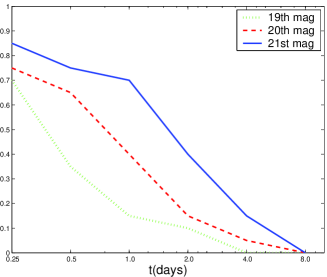
Figure 6: The fraction of bursts with optical afterglow above three limiting magnitudes as a function of time (compared to the total number of bursts with optical afterglow).

Technical difficulties led a gap of several hours between the burst and the detection of the optical afterglow, which could be found only after an accurate position was available. The rapid localization provided by HETE II helped to close this gap and an almost complete light curve from 193 sec after the trigger ($\approx 93$ sec after the end of the burst) is available now for GRB021004 Fox et al. (2003b).

Many afterglow light curves show an achromatic break to a steeper decline with $\alpha\approx 2$. The classical example of such a break was seen in GRB 990510 Harrison et al. (1999); Stanek et al. (1999) and it is shown here in Fig. 7. It is common to fit the break with the phenomenological formula: $F_{\nu}(t)=f_{*}(t/t_{*})^{-\alpha_{1}}\{1-\exp[-(t/t_{*})^{(\alpha_{1}-\alpha_{2})}](t/t_{*})^{(\alpha_{1}-\alpha_{2})}\}$. This break is commonly interpreted as a jet break that allows us to estimate the opening angle of the jet Rhoads (1999); Sari et al. (1999) or the viewing angle within the standard jet model Rossi et al. (2002) (see §II.4 below).

Figure 7: The optical light curves of GRB990510. A fit for the observed optical light curves is obtained with $\alpha_{1}=0.82\pm 0.02$, $\alpha_{2}=2.18\pm 0.05$ and $t_{*}=1.2\pm 0.08$ days (from Harrison et al. (1999)).

The optical light curve of the first detected afterglow (from GRB 970228) could be seen for more than half a year Fruchter et al. (1998). In most cases the afterglow fades faster and cannot be followed for more than several weeks. At this stage the afterglow becomes significantly dimer than its host galaxy and the light curve reaches a plateau corresponding to the emission of the host.

In a several cases: e.g. GRB 980326 Bloom et al. (1999), GRB 970228 Reichart (1999) GRB 011121 Bloom et al. (2002b); Garnavich et al. (2003) red bumps are seen at late times (several weeks to a month). These bumps are usually interpreted as evidence for an underlying SN. A most remarkable Supernova signature was seen recently in GRB 030329 Stanek et al. (2003a); Hjorth et al. (2003). This supernova had the same signature as SN98bw that was associated with GRB 990425 (see §II.3.4).

Finally, I note that varying polarization at optical wavelengths has been observed in GRB afterglows at the level of a few to ten percent Covino et al. (1999); Wijers et al. (1999); Rol et al. (2000); Covino et al. (2002); Bersier et al. (2003); Greiner et al. (2003). These observations are in agreement with rough predictions (Sari (1999b); Ghisellini and Lazzati (1999)) of the synchrotron emission model provided that there is a deviation from spherical symmetry (see §V.6 below).

II.2.3 Dark GRBs

Only $\sim 50\%$ of well-localized GRBs show optical transients (OTs) successive to the prompt gamma-ray emission, whereas an X-ray counterpart is present in 90% of cases (see Fig. 8). Several possible explanations have been suggested for this situation. It is possible that late and shallow observations could not detect the OTs in some cases; several authors argue that dim and/or rapid decaying transients could bias the determination of the fraction of truly obscure GRBs (Fynbo et al., 2001; Berger et al., 2002). However, recent reanalysis of optical observations (Reichart and Yost, 2001; Ghisellini et al., 2001; Lazzati et al., 2002) has shown that GRBs without OT detection (called dark GRBs, FOAs Failed Optical Afterglows, or GHOSTs, Gamma ray burst Hiding an Optical Source Transient) have had on average weaker optical counterparts, at least 2 magnitudes in the R band, than GRBs with OTs. Therefore, they appear to constitute a different class of objects, albeit there could be a fraction undetected for bad imaging.

The nature of dark GRBs is not clear. So far three hypothesis have been put forward to explain the behavior of dark GRBs. First, they are similar to the other bright GRBs, except for the fact that their lines of sight pass through large and dusty molecular clouds, that cause high absorption Reichart and Price (2002). Second, they are more distant than GRBs with OT, at $z\geq 5$ (Fruchter et al., 1999; Lamb and Reichart, 2000), so that the Lyman break is redshifted into the optical band. Nevertheless, the distances of a few dark GRBs have been determined and they do not imply high redshifts (Djorgovski et al., 2001a; Antonelli et al., 2000b; Piro et al., 2002). A third possibility is that the optical afterglow of dark GRBs is intrinsically much fainter (2-3 mag below) than that of other GRBs.

De Pasquale et al. (2002) find that GRBs with optical transients show a remarkably narrow distribution of flux ratios, which corresponds to an average optical-to-x spectral index $0.794\pm 0.054$. They find that, while 75% of dark GRBs have flux ratio upper limits still consistent with those of GRBs with optical transients, the remaining 25% are 4 - 10 times weaker in optical than in X-rays. This result suggests that the afterglows of most dark GRBs are intrinsically fainter in all wavelength relative to the afterglows of GRBs with observed optical transients. As for the remaining 25% here the spectrum (optical to X-ray ratio) must be different than the spectrum of other afterglows with a suppression of the optical band.

II.2.4 Radio afterglow

Radio afterglow was detected in $\sim 50$ % of the well localized bursts. Most observations are done at about 8 GHz since the detection falls off drastically at higher and lower frequencies. The observed peak fluxes are at the level of 2 mJy. A turnover is seen around $0.2$ mJy and the undetected bursts have upper limits of the order of 0.1 mJy. As the localization is based on the X-ray afterglow (and as practically all bursts have X-ray afterglow) almost all these bursts were detected in X-ray . $\sim 80$ % of the radio-afterglow bursts have also optical afterglow. The rest are optically dark. Similarly $\sim 80$% of the optically observed afterglow have also a radio component (see fig 8).

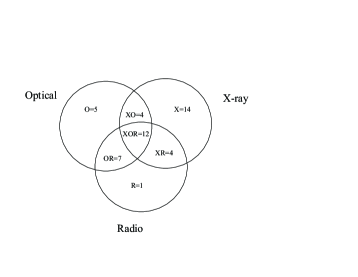
Figure 8: Venn diagram of the distribution of 47 Afterglows observed in different wavelength between 1997-2001 (from a talk given by D. Frail at the Sackler GRB workshop, Harvard, May 2001

Several bursts (GRBs 980329, 990123, 91216, 000926, 001018, 010222, 011030, 011121) were detected at around one day. Recent radio observations begin well before that but do not get a detection until about 24 hrs after a burst. The earliest radio detection took place in GRB 011030 at about 0.8 days after the burst Taylor et al. (2001). In several cases (GRBs 990123, 990506, 991216, 980329 and 020405) the afterglow was detected early enough to indicate emission from the reverse shock and a transition from the reverse shock to the forward shock.

The radio light curve of GRB 970508 (see fig 9) depicts early strong fluctuations (of order unity) in the flux Frail et al. (1997). Goodman (1997) suggested that these fluctuations arise due to scintillations and the decrease (with time) in the amplitude of the fluctuations arises from a transition from strong to weak scintillations. Frail et al. (1997) used this to infer the size of the emitting region of GRB 970508 at $\sim 4$ weeks after the burst as $\sim 10^{17}$cm. This observations provided the first direct proof of relativistic expansion in GRBs.

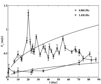
Figure 9: Light curves of the radio afterglow of GRB970508 at 4.86GHz and 1.43GHz, compared with the predictions of the adiabatic fireball model (from Frail et al. (1997)).

The self-absorbed frequencies fall in the centimeter to meter wave radio regime and hence the lower radio emission is within the self-absorption part of the spectrum (see §V.3.3 later). In this case the spectrum rises as $\nu^{2}$ Katz and Piran (1997). The spectral shape that arises from a the fact that the system is optically thick enables us (using similar arguments to those of a simple black body emission) to determine the size of the emitting region. In GRB 990508 this has lead to $\sim 10^{17}$cm. A comparable estimate to the one derived from scintillations.

The long-lived nature of the radio afterglow allows for unambiguous calorimetry of the blast wave to be made when its expansion has become sub-relativistic and quasi-spherical. The light curves evolves on a longer time scale in the radio. Some GRB afterglows have been detected years after the burst even after the relativistic-Newtonian transition (see §VII.4). At this stage the expansion is essentially spherical and this enables a direct ”calorimetric” estimate of the total energy within the ejecta Waxman et al. (1998).

II.3 Hosts and Distribution

II.3.1 Hosts

By now (early 2004) host galaxies have been observed for all but 1 or 2 bursts with optical, radio or X-ray afterglow localization with arcsec precision Hurley et al. (2002e). The no-host problem which made a lot of noise in the nineties has disappeared. GRBs are located within host galaxies (see Djorgovski et al. (2001b, d) and Hurley et al. (2002e) for detailed reviews). While many researchers believe that the GRB host population seem to be representative of the normal star-forming field galaxy population at a comparable redshifts, others argue that GRB host galaxies are significantly bluer than average and their star formation rate is much higher than average.

The host galaxies are faint with median apparent magnitude $R\approx 25$. Some faint hosts are at $R\approx 29$. Down to $R\approx 25$ the observed distribution is consistent with deep field galaxy counts. Jimenez et al. (2001) find that the likelihood of finding a GRB in a galaxy is proportional to the galaxy’s luminosity.

The magnitude and redshift distribution of GRB host galaxies are typical for normal, faint field galaxies, as are their morphologies Odewahn et al. (1998); Holland (2001); Bloom et al. (2002a); Hurley et al. (2002e); Djorgovski et al. (2001d). While some researchers argue that the broad band optical colors of GRB hosts are not distinguishable from those of normal field galaxies at comparable magnitudes and redshifts Bloom et al. (2002a); Sokolov et al. (2001), others Fruchter et al. (1999) asserts that the host galaxies are unusually blue and that they are strongly star forming. Le Floc’h et al. (2003) argues that R-K colors of GRB hosts are unusually blue and the hosts may be of low metallicity and luminosity. This suggests Le Floc’h (2004) that the hosts of GRBs might be different from the cites of the majority of star forming galaxies that are luminous, reddened and dust-enshrouded infrared starbursts (Elbaz and Cesarsky (2003) and references therein). Le Floc’h (2004) also suggests that this difference might rise due to an observational bias and that GRBs that arise in dust-enshrouded infrared starbursts are dark GRBs whose afterglow is not detectable due to obscuration. Whether this is tru or not is very relevant to the interesting question to which extend GRBs follow the SFR and to which extend they can be used to determine the SFR at high redshifts.

Totani (1997), Wijers et al. (1998) and Paczynski (1998) suggested that GRBs follow the star formation rate. As early as 1998 Fruchter et al. (1999) noted that all four early GRBs with spectroscopic identification or deep multicolor broadband imaging of the host (GRB 970228 GRB 970508, GRB 971214, and GRB 980703) lie in rapidly star-forming galaxies. Within the host galaxies the distribution of GRB-host offset follows the light distribution of the hosts Bloom et al. (2002a). The light is roughly proportional to the density of star formation. Spectroscopic measurements suggest that GRBs are within Galaxies with a higher SFR. However, this is typical for normal field galaxy population at comparable redshifts Hurley et al. (2002a). There are some intriguing hints, in particular the flux ratios of [Ne III] 3859 to [OII] 3727 are on average a factor of 4 to 5 higher in GRB hosts than in star forming galaxies at low redshifts Djorgovski et al. (2001d). This may represent an indirect evidence linking GRBs with massive star formation. The link between GRBs and massive stars has been strengthened with the centimeter and submillimeter discoveries of GRB host galaxies Berger et al. (2001); Frail et al. (2002) undergoing prodigious star formation (SFR$\sim 10^{3}$ M_⊙ yr^-1), which remains obscured at optical wavelengths.

Evidence for a different characteristics of GRB host galaxies arise from the work of Fynbo et al. (2002, 2003) who find that GRB host galaxies “always” show Lyman alpha emission in cases where a suitable search has been conducted. This back up the claim for active star formation and at most moderate metallicity in GRB hosts. It clearly distinguishes GRB hosts from the Lyman break galaxy population, in which only about 1/4 of galaxies show strong Lyman alpha.

II.3.2 The Spatial Distribution

BATSE’s discovery that the bursts are distributed uniformly on the sky Meegan et al. (1992) was among the first indication of the cosmological nature of GRBs. The uniform distribution indicated that GRBs are not associated with the Galaxy or with “local” structure in the near Universe.

Recently there have been several claims that sub-groups of the whole GRB population shows a deviation from a uniform distribution. Mészáros et al. (2000b, a), for example, find that the angular distribution of the intermediate sub-group of bursts (more specifically of the weak intermediate sub-group) is not random. Magliocchetti et al. (2003) reported that the two-point angular correlation function of 407 short BATSE GRBs reveal a $\sim 2\sigma$ deviation from isotropy on angular scales $2^{o}-4^{o}$. This results is consistent with the possibility that observed short GRBs are nearer and the angular correlation is induced by the large scale structure correlations on this scale. These claims are important as they could arise only if these bursts are relatively nearby. Alternatively this indicates repetition of these sources Magliocchetti et al. (2003). Any such deviation would imply that these sub-groups are associated with different objects than the main GRB population at least that these subgroup are associated with a specific feature, such as a different viewing angle.

Cline et al. (2003) studied the shortest GRB population, burst with a typical durations several dozen ms. They find that there is a significant angular asymmetry and the $\langle V/V_{max}\rangle$ distribution provides evidence for a homogeneous sources distribution. They suggest that these features are best interpreted as sources of a galactic origin. However, one has to realize that there are strong selection effects that are involved in the detection of this particular subgroup.

II.3.3 GRB rates and the isotropic luminosity function

There have been many attempts to determine the GRB luminosity function and rate from the BATSE peak flux distribution. This was done by numerous using different levels of statistical sophistication and different physical assumptions on the evolution of the rate of GRBs with time and on the shape of the luminosity function.

Roughly speaking the situation is the following. There are now more than 30 redshift measured. The median redshift is $z\approx 1$ and the redshift range is from 0.16 (or even 0.0085 if the association of GRB 980425 with SN 98bw should be also considered) to 4.5 (for GRB 000131). Direct estimates from the sample of GRBs with determined redshifts are contaminated by observational biases and are insufficient to determine the rate and luminosity function. An alternative approach is to estimates these quantities from the BATSE peak flux distribution. However, the observed sample with a known redshifts clearly shows that the luminosity function is wide. With a wide luminosity function, the rate of GRB is only weakly constraint by the peak flux distribution. The analysis is further complicated by the fact that the observed peak luminosity, at a given detector with a given observation energy band depends also on the intrinsic spectrum. Hence different assumptions on the spectrum yield different results. This situation suggest that there is no point in employing sophisticated statistical tools (see however, Loredo and Wasserman (1995); Piran (1999) for a discussion of these methods) and a simple analysis is sufficient to obtain an idea on the relevant parameters.

I will not attempt to review the various approaches here. A partial list of calculations includes Piran (1992); Cohen and Piran (1995); Fenimore and Bloom (1995); Loredo and Wasserman (1995); Horack and Hakkila (1997); Loredo and Wasserman (1998); Piran (1999); Schmidt (1999, 2001a, 2001b); Sethi and Bhargavi (2001). Instead I will just quote results of some estimates of the rates and luminosities of GRBs. The simplest approach is to fit $\langle V/V_{max}\rangle$, which is the first moment of the peak flux distribution. Schmidt (1999, 2001a, 2001b) finds using $\langle V/V_{max}\rangle$ of the long burst distribution and assuming that the bursts follow the Porciani and Madau (2001) SFR2, that the present local rate of long observed GRBs is $\approx~{}0.15{\rm Gpc}^{-3}{\rm yr}^{-1}$ Schmidt (2001a). Note that this rate from Schmidt (2001a) is smaller by a factor of ten than the earlier rate of Schmidt (1999)! This estimate corresponds to a typical (isotropic) peak luminosity of $\sim 10^{51}$ergs/sec. These are the observed rate and the isotropic peak luminosity.

Recently Guetta et al. (2003b) have repeated these calculations . They use both the Rowan-Robinson (1999) SFR formation rate:

$$R_{GRB}(z)=\rho_{0}\left\{\begin{array}[]{ll}10^{0.75z}&z<1\\ 10^{0.75z_{\rm peak}}&z>1.\end{array}\right.\;,$$

and SFR2 from Porciani and Madau (2001). Their best fit luminosity function (per logarithmic luminosity interval, $d\log L$) is:

$$\Phi_{o}(L)=c_{o}\left\{\begin{array}[]{ll}(L/L^{*})^{\alpha}&L^{*}/30<L<L^{*}\\ (L/L^{*})^{\beta}&L^{*}erg/sec<L<30L^{*}\end{array}\right.;,$$ (2)

and 0 otherwise with a typical luminosity, $L^{*}=1.1\times 10^{51}$ergs/sec, $\alpha=-0.6$ and $\beta=-2$, and $c_{o}$ is a normalization constant so that the integral over the luminosity function equals unity. The corresponding local GRB rate is $\rho_{0}=0.44$Gpc^-1yr^-1. There is an uncertainty of a factor of $\sim 2$ in the typical energy, $L^{*}$, and in the local rate. I will use these numbers as the “canonical” values in the rest of this review.

The observed (BATSE) rate of short GRBs is smaller by a factor of three than the rate of long ones. However, this is not the ratio of the real rates as :(i) The BATSE detector is less sensitive to short bursts than to long ones; (ii) The true rate depends on the spatial distribution of the short bursts. So far no redshift was detected for any short bursts and hence this distribution is uncertain. For short bursts we can resort only to estimates based on the peak flux distribution. There are indications that $\langle V/V_{max}\rangle$ of short burst is larger (and close to the Eucleadian value of 0.5) than the $\langle V/V_{max}\rangle$ value of long ones (which is around 0.32). This implies that the observed short bursts are nearer to us that the long ones Mao et al. (1994); Katz and Canel (1996); Tavani (1998) possible with all observed short bursts are at $z<0.5$. However, Schmidt (2001a) finds for short bursts $\langle V/V_{max}\rangle=0.354$, which is rather close to the value of long bursts. Assuming that short GRBs also follow the SFR he obtains a local rate of $0.075{\rm Gpc}^{-3}{\rm yr}^{-1}$ - a factor of two below the rate of long GRBs! The (isotropic) peak luminosities are comparable. This results differs from a recent calculation of Guetta and Piran (2003) who find for short bursts $\langle V/V_{max}\rangle=0.390$ and determine from this a local rate of $1.7{\rm Gpc}^{-3}{\rm yr}^{-1}$ which is about four times the rate of long bursts. This reflects the fact that the observed short GRBs are significantly nearer than the observed long ones.

These rates and luminosities are assuming that the bursts are isotropic. Beaming reduces the actual peak luminosity increases the implied rate by a factor $f_{b}^{-1}=2/\theta^{2}$. By now there is evidence that GRBs are beamed and moreover the total energy in narrowly distributed Frail et al. (2001); Panaitescu and Kumar (2001). There is also a good evidence that the corrected peak luminosity is much more narrowly distributed than the isotropic peak luminosity van Putten and Regimbau (2003); Guetta et al. (2003b). The corrected peak luminosity is $L_{peak}(\theta^{2}/2)\sim const$. Frail et al. (2001) suggest that the true rate is larger by a factor of 500 than the observed isotropic estimated rate. However, Guetta et al. (2003b) repeated this calculation performing a careful average over the luminosity function and find that that true rate is only a factor of $\sim 75\pm 25$ times the isotropically estimate one. Over all the true rate is: $33\pm 11h_{65}^{3}{\rm Gpc}^{-3}{\rm yr}^{-1}$.

With increasing number of GRBs with redshifts it may be possible soon to determine the GRB redshift distribution directly from this data. However, it is not clear what are the observational biases that influence this data set and one needs a homogenous data set in order to perform this calculation. Alternatively one can try to determine luminosity estimators Norris et al. (2000); Fenimore and Ramirez-Ruiz (2001); Schaefer et al. (2001); Schaefer (2003) from the subset with known redshifts and to obtain, using them a redshift distribution for the whole GRB sample. Lloyd-Ronning et al. (2002) find using the Fenimore and Ramirez-Ruiz (2001) sample that this method implies that (i) The rate of GRBs increases backwards with time even for $z>10$, (ii) The Luminosity of GRBs increases with redshift as $(1+z)^{1.4\pm 0.5}$; (iii) Hardness and luminosity are strongly correlated. It is not clear how these features, which clearly depend on the inner engine could depend strongly on the redshift. Note that in view of the luminosity-angle relation (see §II.4 below) the luminosity depends mostly on the opening angle. An increase of the luminosity with redshift would imply that GRBs were more narrowly collimated at earlier times.

II.3.4 Association with Supernovae

The association of GRBs with star forming regions and the indications that GRBs follow the star formation rate suggest that GRBs are related to stellar death, namely to Supernovae Paczynski (1998). Additionally there is some direct evidence of association of GRBs with Supernovae.

GRB 980425 and SN98bw: The first indication of an association between GRBs and SNes was found when SN 98bw was discovered within the error box of GRB 980425 Galama et al. (1998). This was an usual type Ic SN which was much brighter than most SNs. Typical ejection velocities in the SN were larger than usual ($\sim 2\cdot 10^{4}km/sec$) corresponding to a kinetic energy of $2-5^{52}$ ergs, more than ten times than previously known energy of SNes, Iwamoto et al. (1998). Additionally radio observations suggested a component expanding sub relativistically with $v\sim 0.3c$ Kulkarni et al. (1998). Thus, 1998bw was an unusual type Ic supernovae, significantly more powerful than comparable SNes. This may imply that SNs are associated with more powerful SNes. Indeed all other observations of SN signature in GRB afterglow light curves use a SN 98bw templates. The accompanying GRB, 980425 was also unusual. GRB 980425 had a smooth FRED light curve and no high energy component in its spectrum. Other bursts like this exist but they are rare. The redshift of SN98bw was 0.0085 implying an isotropic equivalent energy of $\sim 10^{48}$ergs. Weaker by several orders of magnitude than a typical GRB.

The BeppoSAX Wide Field Cameras had localized GRB980425 with a 8 arcmin radius accuracy. In this circle, the BeppoSAX NFI (Narrow Field Instrument) had detected two sources, S1 and S2. The NFI could associate with each of these 2 sources an error circle of 1.5 arcmin radius. The radio and optical position of SN1998bw were consistent only with the NFI error circle of S1, and was out of the NFI error circle of S2. Therefore, Pian et al. (2000) identified S1 with X-ray emission from SN1998bw, although this was of course no proof of association between SN and GRB. It was difficult, based only on the BeppoSAX NFI data, to characterize the behavior and variability of S2 and it could not be excluded that S2 was the afterglow of GRB980425. The XMM observations of March 2002 Pian et al. (2003) seem to have brought us closer to the solution. XMM detects well S1, and its flux is lower than in 1998: the SN emission has evidently decreased. Concerning the crucial issue, S2: XMM, having a better angular resolution than BeppoSAX NFIs, seems to resolve S2 in a number of sources. In other words, S2 seems to be not a single source, but a group of small faint sources. Their random variability (typical fluctuations of X-ray sources close to the level of the background) may have caused the flickering detected for S2. This demolishes the case for the afterglow nature of S2, and strengthens in turn the case for association between GRB980425 and SN1998bw.

Red Bumps: The late red bumps (see §II.2.2) have been discovered in several GRB light curves Bloom et al. (1999); Reichart (1999); Bloom et al. (2002b); Garnavich et al. (2003). These bumps involve both a brightening (or a flattening) of the afterglow as well as a transition to a much redder spectrum. These bumps have been generally interpreted as due to an underlining SN Bloom et al. (1999). In all cases the bumps have been fit with a template of SN 1998bw, which was associated with GRB 980425. Esin and Blandford (2000) proposed that these bumps are produced by light echoes on surrounding dust (but see Reichart (2001)). Waxman and Draine (2000) purposed another alternative explanation based on dust sublimation.

For most GRBs there is only an upper limit to the magnitude of the bump in the light curve. A comparison of these upper limits (see Fig. 10) with the maximal magnitudes of type Ibc SNe shows that the faintest GRB-SN non-detection (GRB 010921) only probes the top $\sim$40th-percentile of local Type Ib/Ic SNe. It is clear that the current GRB-SNe population may have only revealed the tip of the iceberg; plausibly, then, SNe could accompany all long-duration GRBs.

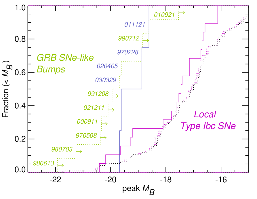
Figure 10: Comparison of the peak magnitudes of GRB-SNe with those of local Type Ib/Ic SNe. The solid cumulative histogram to the left is for those GRBs with a believable detection of a SN bump; the brightness of all other claimed GRB-SN peaks or reported upper-limits are shown as a dotted histogram. The solid histogram to the right is for those local Ibc SNe for which the SN was observed before peak; all others were discovered after peak. The faintest GRB-SN non-detection (010921) only probes the top $\sim$40th-percentile of local Type Ib/Ic SNe. It is clear that the current GRB-SNe population may have only revealed the tip of the iceberg; plausibly, then, SNe could accompany all long-duration GRBs, from Bloom (2003)

GRB 030329 and CN 2003dh: The confirmation of SN 98bw like bump and the confirmation of the GRB-SN association was dramatically seen recently Stanek et al. (2003b); Hjorth et al. (2003) in the very bright GRB 030329 that is associated with SN 2003dh Chornock et al. (2003). The bump begun to be noticed six days after the bursts and the SN 1999bw like spectrum dominated the optical light curve at later times (see Fig. 11. The spectral shapes of 2003dh and 1998bw were quite similar, although there are also differences. For example II.4 estimated a somewhat larger expansion velocity for 2003dh. Additionally the X-ray signal was much brighter (but this could be purely afterglow).

For most researchers in the field this discovery provided the final conclusive link between SNe and GRBs (at least with long GRBs). As the SN signature coincides with the GRB this observations also provides evidence against a Supranova interpretation, in which the GRB arises from a collapse of a Neutron star that takes place sometime after the Supernova in which the Neutron star was born - see IX.5 . (unless there is a variety of Supranova types, some with long delay and others with short delay between the first and the second collapses) the spectral shapes of 2003dh and 1998bw were quite similar, although there are also differences. For example there is a slightly larger expansion velocity for 2003dh. It is interesting that while not as week as GRB 990425, the accompanying GRB 99030329 was significantly weaker than average. The implied opening angle reveals that the prompt $\gamma$-ray energy output, $E_{\gamma}$, and the X-ray luminosity at $10\;$hr, $L_{X}$, are a factor of $\sim 20$ and $\sim 30$, respectively, below the average value around which most GRBs are narrowly clustered (see II.4 below).

Figure 11: Evolution of the GRB 030329/SN2004dh spectrum, from April 1.13 UT (2.64 days after the burst), to April 8.13 UT (6.94 days after the burst). The early spectra consist of a power law continuum ($F_{\nu}\propto\nu^{-0.9}$) with narrow emission lines originating from HII regions within the host galaxy at redshift z=0.168. Spectra taken after April 5 show the development of broad peaks characteristic of a supernova (from Stanek et al. (2003b).

It is interesting to compare SN 1999bw and SN 2003dh. Basically, at all epochs Matheson et al. (2003) find that the best fit to spectra of 2003dh is given by 1998bw at about the same age . The light curve is harder, as the afterglow contribution is significant, but using spectral information they find that 2003dh had basically the same light curve as 1998bw. Mazzali et al. (2003) model the spectra and find again that it was very similar to 1998bw. They find some differences, but some of that might be due to a somewhat different approach to spectral decomposition, which gives somewhat fainter supernova.

X-ray lines: The appearance of iron X-ray lines (see §II.2.1) has been interpreted as additional evidence for SN. One has to be careful with this interpretation as the iron X-ray lines are seen as if emitted by matter at very low velocities and at rather large distances. This is difficult to achieve if the supernova is simultaneous with the GRB, as the SN bumps imply. This X-ray lines might be consistent with the Supranova model Vietri and Stella (1998) in which the SN takes place month before the GRB. However, in this case there won’t be a SN bump in the light curve! Rees and Mészáros (2000); Mészáros and Rees (2001a) and Kumar and Narayan (2003) suggest alternative interpretations which do not require a Supranova.

II.4 Energetics

Before redshift measurements were available the GRB energy was estimated from the BATSE catalogue by fitting an (isotropic) luminosity function to the flux distribution (see e.g Cohen and Piran (1995); Loredo and Wasserman (1998); Schmidt (1999, 2001a, 2001b); Guetta et al. (2003b) and many others). This lead to a statistical estimate of the luminosity function of a distribution of bursts.

These estimates were revolutionized with the direct determination of the redshift for individual bursts. Now the energy could be estimated directly for specific bursts. Given an observed $\gamma$-ray fluence and the redshift to a burst one can easily estimate the energy emitted in $\gamma$-rays, $E_{\gamma,iso}$ assuming that the emission is isotropic (see Bloom et al. (2001) for a detailed study including k corrections). The inferred energy, $E_{\gamma,iso}$ was the isotropic energy, namely the energy assuming that the GRB emission is isotropic in all directions. The energy of the first burst with a determined redshift, GRB 970508, was around $10^{51}$ergs. However, as afterglow observations proceeded, alarmingly large values (e.g. $3.4\times 10^{54}$ergs for GRB990123) were measured for $E_{\gamma,iso}$. The variance was around three orders of magnitude.

However, it turned out Rhoads (1999); Sari et al. (1999) that GRBs are beamed and $E_{\gamma,iso}$ would not then be a good estimate for the total energy emitted in $\gamma$-rays. Instead: $E_{\gamma}\equiv(\theta^{2}/2)E_{\gamma,iso}$. The angle, $\theta$, is the effective angle of $\gamma$-ray emission. It can be estimated from $t_{b}$, the time of the break in the afterglow light curve Sari et al. (1999):

$$\theta=0.16(n/E_{k,iso,52})^{1/8}t_{b,days}^{3/8}=0.07(n/E_{k,\theta,52})^{1/6}t_{b,days}^{1/2},$$ (3)

where $t_{b,days}$ is the break time in days. $E_{k,iso,52}$ is “isotropic equivalent” kinetic energy, discussed below, in units of $10^{52}$ergs, while $E_{k,\theta,52}$ is the real kinetic energy in the jet i.e: $E_{k,\theta,52}=(\theta^{2}/2)E_{k,iso,52}$. One has to be careful which of the two energies one discusses. In the following I will usually consider, unless specifically mentioned differently, $E_{k,iso,52}$, which is also related to the energy per unit solid angle as: $E_{k,iso,52}/4\pi$. The jet break is observed both in the optical and in the radio frequencies. Note that the the observational signature in the radio differs from that at optical and X-ray Sari et al. (1999); Harrison et al. (1999) (see Fig. 25) and this provides an additional confirmation for this interpretation.

Frail et al. (2001) estimated $E_{\gamma}$ for 18 bursts, finding typical values around $10^{51}$ergs (see also Panaitescu and Kumar (2001)). Bloom et al. (2003) find ${E}_{\gamma}=1.33\times 10^{51}\,h_{65}^{-2}$ erg and a burst–to–burst variance about this value $\sim 0.35$ dex, a factor of 2.2. This is three orders of magnitude smaller than the variance in the isotropic equivalent $E_{\gamma}$. A compilation of the beamed energies from Bloom et al. (2003), is shown in Figs 12 and 13. It demonstrates nicely this phenomenon. The constancy of $E_{\gamma}$ is remarkable, as it involves a product of a factor inferred from the GRB observation (the $\gamma$-rays flux) with a factor inferred from the afterglow observations (the jet opening angle). However, $E_{\gamma}$ might not be a good estimate for $E_{tot}$, the total energy emitted by the central engine. First, an unknown conversion efficiency of energy to $\gamma$-rays has to be considered: $E_{tot}=\epsilon^{-1}E_{\gamma}=\epsilon^{-1}(\theta^{2}/2)E_{\gamma,iso}$. Second, the large Lorentz factor during the $\gamma$-ray emission phase, makes the observed $E_{\gamma}$ rather sensitive to angular inhomogeneities of the relativistic ejecta Kumar and Piran (2000a). The recent early observations of the afterglow of GRB 021004 indicate that indeed a significant angular variability of this kind exists Nakar et al. (2003b); Nakar and Piran (2003a).

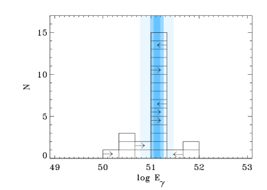
Figure 12: A histogram of GRB energies ($E_{\gamma}$) with three equal logarithmic spacings per decade. The histogram shows a narrow distribution of GRB energies about the standard energy ${E}_{\gamma}=1.33\cdot 10^{51}$ ergs , with an error of $\sigma=0.07$ dex. The observed burst–to–burst rms spread is $0.35$ dex (a factor of 2.23) about this value. Bands of 1, 2, and 5 $\sigma$ about the standard energy are shown. There are five identifiable outliers, which lie more than 5 $\sigma$ from the mean, however, there is currently no basis other than discrepant energy to exclude these bursts from the sample (Bloom et al. (2003).

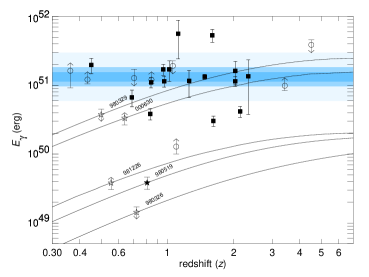
Figure 13: GRB energy release versus redshift. Bands of 1, 2, and 5 $\sigma$ about the mean energy ${E}_{\gamma}=1.33\cdot 10^{51}$ ergs are shown. Plotted are the trajectories of five GRBs with no known spectroscopic redshift (labeled with star symbols). While the energies of GRB 980329 and GRB 000630 could be consistent with the standard value at redshifts beyond $z\sim 1.5$, at no redshift could the energies of GRB 980326 and GRB 980519 be consistent citeBloomFrailKulkarni03.

The kinetic energy of the flow during the adiabatic afterglow phase, $E_{k}$ is yet another energy measure that arises. This energy (per unit solid angle) can be estimated from the afterglow light curve and spectra. Specifically it is rather closely related to the observed afterglow X-ray flux Kumar (2000); Freedman and Waxman (2001); Piran et al. (2001). As this energy is measured when the Lorentz factor is smaller it is less sensitive than $E_{\gamma}$ to angular variability. The constancy of the X-ray flux Piran et al. (2001) suggest that this energy is also constant. Estimates of $E_{k,\theta}$ Panaitescu and Kumar (2001) show that $\bar{E}_{\gamma}\approx 3\bar{E}_{k,\theta}$, namely the observed “beamed” GRB energy is larger than the estimated “beamed” kinetic energy of the afterglow. Frail et al. (2001), however, find that $\bar{E}_{\gamma}\approx\bar{E}_{k,\theta}$, namely that the two energies are comparable.

An alternative interpretation to the observed breaks is that we are viewing a “universal” angle dependent, namely, “structured” jet - from different viewing angles Lipunov et al. (2001); Rossi et al. (2002); Zhang and Mészáros (2002). The observed break corresponds in this model to the observing angle $\theta$ and not to the opening angle of the jet. This interpretation means that the GRB beams are wide and hence the rate of GRBs is smaller than the rate implied by the usual beaming factor. On the other hand it implies that GRBs are more energetic. Guetta et al. (2003b) estimate that this factor (the ratio of the fixed energy of a “structured” jet relative to the energy of a uniform jet to be $\sim 7$. However they find that the observing angle distribution is somewhat inconsistent with the simple geometric one that should arise in universal structured jets (see also Perna et al. (2003); Nakar et al. (2003a)). The energy-angle relation discussed earlier require (see §VII.9 below) an angle dependent jet with $E(\theta)\propto\theta^{-2}$.

Regardless of the nature of the jet (universal structured jet or uniform with a opening angle that differs from one burst to another) at late time it becomes non relativistic and spherical. With no relativistic beaming every observer detects emission from the whole shell. Radio observations at this stage enable us to obtain a direct calorimetric estimate of the total kinetic energy of the ejecta at late times Frail et al. (2000b) Estimates performed in several cases yield a comparable value for the total energy.

If GRBs are beamed we should expect orphan afterglows (see §VII.11): events in which we will miss the GRB but we will observe the late afterglow that is not so beamed. A comparison of the rate of orphan afterglows to GRBs will give us a direct estimate of the beaming of GRBs (and hence of their energy). Unfortunately there are not even good upper limits on the rate of orphan afterglows. Veerswijk (2003) consider the observations within the Faint Sky Variability Survey (FSVS) carried out on the Wide Field Camerea on teh 2.5-m Isacc Newton Telescope on La Palma. This survey mapped 23 suare degree down to a limiting magnitude of about V=24. They have found one object which faded and was not detected after a year. However, its colors suggest that it was a supernova and not a GRB. Similarly, Vanden Berk et al. (2002) find a single candidate within the Sloan Digital Sky Survey. Here the colors were compatible with an afterglow. However, later it was revealed that this was a variable AGN and not an orphan afterglow. As I discuss later this limits are still far to constrain the current beaming estimates (see §VII.11).

One exception is for late radio emission for which there are some limits Perna and Loeb (1998); Levinson et al. (2002). Levinson et al. (2002) show that the number of orphan radio afterglows associated with GRBs that should be detected by a flux-limited radio survey is smaller for a smaller jet opening angle $\theta$. This might seen at first sight contrary to expectation as narrower beams imply more GRBs. But, on the other hand, with narrower beams each GRB has a lower energy and hence its radio afterglow is more difficult to detect. Overall the second factor wins. Using the results of FIRST and NVSS surveys they find nine afterglow candidates. If all candidates are associated with GRBs then there is a lower limit on the beaming factor of $f^{-1}_{b}\equiv(\theta^{2}/2)>13$. If none are associated with GRBs they find $f^{-1}_{b}>90$. This give immediately a corresponding upper limit on the average energies of GRBs. Guetta et al. (2003b) revise this values in view of a recent estimates of the correction to the rate of GRBs to: $f^{-1}_{b}=40$.

When considering the energy of GRBs one has to remember the possibility, as some models suggest, that an additional energy is emitted which is not involved in the GRB itself or in the afterglow. van Putten and Levinson (2001), for example, suggest that a powerful Newtonian wind collimates the less powerful relativistic one. The “standard jet” model also suggests a large amount of energy emitted sideways with a lower energy per solid angle and a lower Lorentz factors. It is interesting to note that the calorimetric estimates mentioned earlier limit the total amount of energy ejected regardless of the nature of the flow. More generally, typically during the afterglow matter moving with a lower Lorentz factor emits lower frequencies. Hence by comparing the relative beaming of afterglow emission in different wavelength one can estimate the relative beaming factors, $f^{-1}_{b}(E)$, at different wavelength and hence at different energies. Nakar and Piran (2003b) use various X-ray searches for orphan X-ray afterglow to limit the (hard) X-ray energy to be at most comparable to the $\gamma$-rays energy. This implies that the total energy of matter moving at a Lorentz factor of $\sim 40$ is at most comparable to the energy of matter moving with a Lorentz factor of a few hundred and producing the GRB itself. At present limits on optical orphan afterglow are insufficient to set significant limits on matter moving at slower rate, while as mentioned earlier radio observations already limit the overall energy output.

These observations won’t limit, of course, the energy emitted in gravitational radiation, neutrinos, Cosmic Rays or very high energy photons that may be emitted simultaneously by the source and influence the source’e energy budget without influencing the afterglow.

III THE GLOBAL PICTURE - GENERALLY ACCEPTED INGREDIENTS

There are several generally accepted ingredients in practically all current GRB models.

Relativistic Motion: Practically all current GRB models involve a relativistic motion with a Lorentz factor, $\Gamma>100$. This is essential to overcome the compactness problem (see §IV.1 below). At first this understanding was based only on theoretical arguments. However, now there are direct observational proofs of this concept: It is now generally accepted that both the radio scintillation Goodman (1997) and the lower frequency self-absorption Katz and Piran (1997) provide independent estimates of the size of the afterglow, $\sim 10^{17}$cm, two weeks after the burst. These observations imply that the afterglow has indeed expanded relativistically. Sari and Piran (1999b) suggested that the optical flash accompanying GRB 990123 provided a direct evidence for ultra-relativistic motion with $\Gamma\sim 100$. Soderberg and Ramirez-Ruiz (2003) find a higher value: $1000\pm 100$. However, these interpretations are model dependent.

The relativistic motion implies that we observe blue shifted photons which are significantly softer in the moving rest frame. It also implies that when the objects have a size $R$ the observed emission arrives on a typical time scale of $R/c\Gamma^{2}$ (see §IV.2). Relativistic beaming also implies that we observe only a small fraction ($1/\Gamma$) of the source. As I discussed earlier (see §II.4 and also IV.3) this has important implications on our ability to estimate the total energy of GRBs.

While all models are based on ultra-relativistic motion, none explains convincingly (this is clearly a subjective statement) how this relativistic motion is attained. There is no agreement even on the nature of the relativistic flow. While in some models the energy is carried out in the form of kinetic energy of baryonic outflow in others it is a Poynting dominated flow or both.

Dissipation In most models the energy of the relativistic flow is dissipated and this provides the energy needed for the GRB and the subsequent afterglow. The dissipation is in the form of (collisionless) shocks, possibly via plasma instability. There is a general agreement that the afterglow is produced via external shocks with the circumburst matter (see VII). There is convincing evidence (see e.g. Fenimore et al. (1996); Sari and Piran (1997b); Ramirez-Ruiz and Fenimore (2000); Piran and Nakar (2002) and §VI.1 below) that in most bursts the dissipation during the GRB phase takes place via internal shocks, namely shocks within the relativistic flow itself. Some (see e.g. Dermer and Mitman (1999); Heinz and Begelman (1999); Ruffini et al. (2001); Dar (2003)) disagree with this statement.

Synchrotron Radiation: Most models (both of the GRB and the afterglow) are based on Synchrotron emission from relativistic electrons accelerated within the shocks. There is a reasonable agreement between the predictions of the synchrotron model and afterglow observations Wijers and Galama (1999a); Granot et al. (1999a); Panaitescu and Kumar (2001). These are also supported by measurements of linear polarization in several optical afterglows (see §II.2.2). As for the GRB itself there are various worries about the validity of this model. In particular there are some inconsistencies between the observed special slopes and those predicted by the synchrotron model (see Preece et al. (2002) and §II.1.1). The main alternative to Synchrotron emission is synchrotron-self Compton Waxman (1997b); Ghisellini and Celotti (1999) or inverse Compton of external light Shemi (1994); Brainerd (1994); Shaviv and Dar (1995); Lazzati et al. (2003). The last model requires, of course a reasonable source of external light.

Jets and Collimation: Monochromatic breaks appear in many afterglow light curves. These breaks are interpreted as “jet breaks” due to the sideways beaming of the relativistic emission Panaitescu and Mészáros (1999); Rhoads (1999); Sari et al. (1999) (when the Lorentz factor drops below $1/\theta_{0}$ the radiation is beamed outside of the original jet reducing the observed flux) and due to the sideways spreading of a beamed flow Rhoads (1999); Sari et al. (1999). An alternative interpretation is of a viewing angles of a “universal structured jet” Lipunov et al. (2001); Rossi et al. (2002); Zhang and Mészáros (2002) whose energy varies with the angle. Both interpretations suggest that GRBs are beamed. However, they give different estimates of the overall rate and the energies of GRBs (see §VII.9 below). In either case the energy involved with GRBs is smaller than the naively interpreted isotropic energy and the rate is higher than the observed rate.

A (Newborn) Compact Object If one accepts the beaming interpretation of the breaks in the optical light curve the total energy release in GRBs is $\sim 10^{51}$ergs Frail et al. (2001); Panaitescu and Kumar (2001). It is higher if, as some models suggest, the beaming interpretation is wrong or if a significant amount of additional energy (which does not contribute to the GRB or to the afterglow) is emitted from the source. This energy, $\sim 10^{51}$ergs, is comparable to the energy released in a supernovae. It indicates that the process must involve a compact object. No other known source can release so much energy within such a short time scale. The process requires a dissipation of $\sim 0.1m_{\odot}$ within the central engine over a period of a few seconds. The sudden appearance of so much matter in the vicinity of the compact object suggest a violent process, one that most likely involves the birth of the compact object itself.

Association with Star Formation and SNe: Afterglow observations, which exist for a subset of relatively bright long bursts, show that GRBs arise within galaxies with a high star formation rate (see Djorgovski et al. (2001c) and §II.3.1). Within the galaxies the bursts distribution follows the light distribution Bloom et al. (2002a). This has lead to the understanding that (long) GRB arise from the collapse of massive stars (see §IX.4). This understanding has been confirmed by the appearance of SN bumps in the afterglow light curve (see §II.3.4 earlier) and in particular by the associations of SN 1999bw with GRB 980425 and of SN 2003dh with GRB 030329.

Summary: Based on these generally accepted ideas one can sketch the following generic GRB model: GRBs are a rare phenomenon observed within star forming regions and associated with the death of massive stars and the birth of compact objects. The $\gamma$-rays emission arises from internal dissipation within a relativistic flow. This takes place at a distances of $\sim 10^{13}-10^{15}$cm from the central source that produces the relativistic outflow. Subsequent dissipation of the remaining energy due to interaction with the surrounding circumburst matter produces the afterglow. The nature of the “inner engine” is not resolved yet, however, a the association with SN (like 1998bw and 2003dh) shows that long GRBs involve a a collapsing star. Much less is known on the origin of short GRBs.

IV RELATIVISTIC EFFECTS

IV.1 Compactness and relativistic motion

The first theoretical clues to the necessity of relativistic motion in GRBs arose from the Compactness problem Ruderman (1975). The conceptual argument is simple. GRBs show a non thermal spectrum with a significant high energy tail (see §II.1.1). On the other hand a naive calculation implies that the source is optically thick. The fluctuations on a time scale $\delta t$ imply that the source is smaller than $c\delta t$. Given an observed flux $F$, a duration $T$, and an distance $d$ we can estimate the energy $E$ at the source. For a typical photon’s energy $\bar{E}_{\gamma}$ this yields a photon density $\approx 4\pi d^{2}F/\bar{E}_{\gamma}c^{3}\delta t^{2}$. Now, two $\gamma$-rays can annihilate and produce e⁺e^- pairs, if the energy in their CM frame is larger than $2m_{e}c^{2}$. The optical depth for pair creation is:

$$\tau_{\gamma\gamma}\approx{f_{e^{\pm}}\sigma_{T}4\pi d^{2}F\over\bar{E}_{\gamma}c^{2}\delta t}$$ (4)

where, $f_{e^{\pm}}$ is a numerical factor denoting the average probability that photon will collide with another photon whose energy is sufficient for pair creation. For typical values and cosmological distances, the resulting optical depth is extremely large $\tau_{e^{\pm}}\sim 10^{15}$ Piran (1995). This is, of course, inconsistent with the non-thermal spectrum.

The compactness problem can be resolved if the emitting matter is moving relativistically towards the observer. I denote the Lorentz factor of the motion by $\Gamma$. Two corrections appear in this case. First, the observed photons are blue shifted and therefore, their energy at the source frame is lower by a factor $\Gamma$. Second, the implied size of a source moving towards us with a Lorentz factor $\Gamma$ is $c\delta t\Gamma^{2}$ (see §IV.2 below). The first effect modifies $f_{e^{\pm}}$ by a factor $\Gamma^{-2\alpha}$ where $\alpha$ is the photon’s index of the observed $\gamma$-rays (namely the number of observed photons per unit energy is proportional to $E^{-\alpha}$.). The second effect modifies the density estimate by a factor $\Gamma^{-4}$ and it influences the optical depth as $\Gamma^{-2}$. Together one finds that for $\alpha\sim 2$ one needs $\Gamma\gtrsim 100$ to obtain an optically thin source.

The requirement that the source would be optically thin can be used to obtain direct limits from specific bursts on the minimal Lorentz factor within those bursts Krolik and Pier (1991); Fenimore et al. (1993); Woods and Loeb (1995); Piran (1995); Baring and Harding (1997); Piran (1999); Lithwick and Sari (2001). A complete calculation requires a detailed integration over angular integrals and over the energy dependent pair production cross section. The minimal Lorentz factor depends also on the maximal photon energy, $E_{\rm max}$, the upper energy cutoff of the spectrum. Lithwick and Sari (2001) provide a detailed comparison of the different calculations and point our various flaws in some of the previous estimates. They find that:

$$\tau_{\gamma\gamma}={11\over 180}{\sigma_{T}d^{2}(m_{e}c^{2})^{-\alpha+1}{\cal F}\over c^{2}\delta T(\alpha-1)}({E_{\rm max}\over m_{e}c^{2}})^{\alpha-1}\Gamma^{2\alpha+2}(1+z)^{2\alpha-2}\ ,$$ (5)

where the high end of the observed photon flux is given by ${\cal F}E^{-\alpha}$ (photons per cm² per sec per unit photon energy). A lower limit on $\Gamma$ is obtained by equating Eq. 5 to unity.

IV.2 Relativistic time effects

Consider first a source moving relativistically with a constant velocity along a line towards the observer and two photons emitted at $R_{1}$ and $R_{2}$. The first photon (emitted at $R_{1}$) will reach the observer at time $(R_{2}-R_{1})/v-(R_{2}-R_{1})/c$ before the second photon (emitted at $R_{2}$). For $\Gamma\gg 1$ this equals $\approx(R_{2}-R_{1})/2c\Gamma^{2}$. This allows us to associate an “observer time” $R/2c\Gamma^{2}$ with the distance $R$ and for this reason I have associated a scale $c\delta t\Gamma^{-2}$ with fluctuations on a time scale $\delta t$ in the optical depth equation earlier (see §IV.1). This last relation should be modified if the source moves a varying velocity (v=v(R)). Now

$$\delta t_{12}\approx\int_{R_{1}}^{R_{2}}\frac{dR}{2c\Gamma^{2}(R)}\ ,$$ (6)

which reduces to

$$T_{R}\approx R/2c\Gamma^{2}\ ,$$ (7)

for motion with a constant velocity. The difference between a constant velocity source and a decelerating source introduces a numerical factor of order eight which is important during the afterglow phase Sari (1997).

Consider now a relativistically expanding spherical shell, or at least a shell that is locally spherical (on a scale larger than $1/\Gamma$). Emission from parts of the shell moving at angle $\theta$ relative to the line of sight to the observer will arrive later with a time delay $R(1-cos\theta)/c$. For small angles this time delay equals $R\theta^{2}/2c$. As the radiation is beamed with an effective beaming angle $\approx 1/\Gamma$ most of the radiation will arrive within a typical angular time scale:

$$T_{ang}\equiv R/2c\Gamma^{2}\ .$$ (8)

The combination of time delay and blueshift implies that if the emitted spectrum is a power law spectrum with a spectral index $\alpha$ then the observed signal from the instantaneous emission of a thin shell will decay at late time as a power law with $t^{-(2-\alpha)}$ Fenimore et al. (1996); Nakar and Piran (2003b). The observed pulse from an instantaneous flash from a thin shell is shown in Fig. 14.

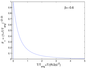
Figure 14: The observed pulse from an instantaneous flash from a spherical relativistic thin shell moving relativistically and emitting emitting with a power low $\nu^{-0.6}$.

As I discuss later (see §VI.1) the similarity between the angular time scale and the radial time scale plays a crucial role in GRB models.

IV.3 Relativistic Beaming and the Patchy Shell Model

The radiation from a relativistic source is beamed with a typical beaming angle $1/\Gamma$. This implies that if the source that is expanding radially with an ultra-relativistic speed a given observer “sees” radiation only from a region that is within $\Gamma^{-1}$ from its line of sight to the source. If the radius of the emitting region is $R$ the observer will see radiation from a region of size $R/\Gamma$. Since $\Gamma$ is extremely large during the GRB we observe emission only from a small fraction of the emitting shell. It is possible, and even likely, that the conditions within the small region that we observe will be different from the average ones across the shell. This means that the conditions that we infer won’t reflect the true average conditions within this particular GRB.

An interesting point related to the internal shocks (discussed later) model in this context is the following. According to the internal shocks model individual pulses are obtained by collisions between individual shells. Here the inhomogeneity of individual shells could be wiped out when the contributions of different hot spots from different shells is added. Alternatively the “inner engine” may produce a consistent angular pattern in which the hot spot is in the same position in all shells and in this case averaging won’t lead to a cancellation of the patchy shell structure.

Within the internal-external model the GRB is produced by internal shocks in which only the relative motion within the flow is dissipated. The bulk Lorentz factor remains unchanged. During the afterglow the shell is slowed down by external shocks. As the Lorentz factor decreases with time (see Eq. VII.1) we observe a larger and larger fraction of the emitting region until $\Gamma\approx\theta^{-1}$, where $\theta$ is the angular size of the whole emitting region - the GRB jet, see §VII.8. This has several inevitable implications. If the initial relativistic flow is inhomogenous on a small angular scale then different observers looking at the same GRB (from different viewing angles) will see different $\gamma$-rays light curves. A strong burst to one observer might look weak to another one if it is located at an angle larger than $1/\Gamma$ from the first. The two observers will see similar conditions later on, during the afterglow, as then they will observe the same angular regions. This has the following implications: (i) Given that the GRB population originate from some ‘typical’ distribution we expect that fluctuation between different bursts at early time during the GRB will be larger than fluctuations observed at late times during the afterglow Kumar and Piran (2000a). A direct consequence of this behaviour is the appearance of a bias in the observations of GRBs. As we are more likely to detect stronger events we will tend to identify bursts in which a ‘hot spot‘ was pointing towards us during the GRB phase. If the original GRB shells are inhomogenous this would inevitably lead to a bias in the estimates of the GRB emission as compared to the kinetic energy during the afterglow. (ii) As the afterglow slows down we observe a larger and larger region. The angular structure would produces a variability in the light curve with a typical time scale of t, the observed time. These fluctuations will decay later as the Lorentz factor decreases and the observations are averaged over a larger viewing angle. Nakar et al. (2003b) have suggested that this is the source of the early fluctuations in the light curve of GRB 021004. Nakar and Oren (2003) modelled this process with a numerical simulation. They find that the flucutation light curve of GRB 021004 can be nicely fitted by this model and that it also explains the correlated fluctuations in the polarization (see also Granot (2003)).

V PHYSICAL PROCESSES

The observed prompt emission must be generated by energetic particles that have been accelerated within the collisionless shocks. The most likely process is synchrotron emission, even though there is some evidence that a simple synchrotron spectra does not fit all bursts Preece et al. (2002) (but see however, Barraud et al. (2003) who finds consistency with the synchrotron model). I consider here, the different physical ingredient that determine the emission process: particle acceleration, magnetic field amplification, synchrotron emission and inverse Compton emission that could be relevant in some cases.

V.1 Relativistic Shocks

Shocks involve sharp jumps in the physical conditions. Conservation of mass, energy and momentum determine the Hugoniot shock jump conditions across the relativistic shocks for the case when the upstream matter is cold (see e.g. Blandford and McKee (1976)):

$$n_{2}=4\Gamma n_{1}$$ (9)

$$e_{2}=4\Gamma n_{1}m_{p}c^{2}$$

$$\Gamma_{sh}^{2}=2\Gamma^{2}$$

where $n_{1,2}$,$e_{1,2}$ are the number density and the energy density (measured in the local rest frame) of the matter upstream (region 1) and downstream (region 2). I have assumed that the energy density in region 1 is very small compared to the rest mass density. $\Gamma$ is the Lorentz factor of the fluid just behind the shock and $\Gamma_{sh}$ is the Lorentz factor of the shock front (both measured in the rest frame of the upstream fluid). The matter is compressed by a factor $\Gamma$ across a relativistic shock. The pressure, or the internal energy density behind the shock is of order $\Gamma^{2}n_{1}m_{p}c^{2}$. Thus, in the shock’s rest frame the relative “thermal” energy per particle (downstream) is of the same order of the kinetic energy per particle (ahead of the shock) upstream. Put differently the shock converts the ‘ordered’ kinetic energy to a comparable random kinetic energy. In an ultra-relativistic shock the downstream random velocities are ultra-relativistic.

Similar jump conditions can be derived for the Magnetic fields across the shock. The parallel magnetic field (parallel to the shock front) $B_{||}$ is compressed and amplified:

$$B_{||2}=\Gamma B_{||1}$$ (10)

The perpendicular magnetic field $B_{\bot}$ remains unchanged.

The energy distribution of the (relativistic) electrons and the magnetic field behind the shock are needed to calculate the Synchrotron spectrum. In principle these parameters should be determined from the microscopic physical processes that take place in the shocks. However, it is difficult to estimate them from first principles. Instead I define two dimensionless parameters, $\epsilon_{B}$ and $\epsilon_{e}$, that incorporate our ignorance and uncertainties Paczynski and Rhoads (1993); Piran (1994); Sari et al. (1996). It is commonly assumed that these energies are a constant fraction of the internal energy behind the shock (see however, Daigne and Mochkovitch (2003)). I denote by $\epsilon_{e}$ and by $\epsilon_{B}$ the ratio between these energies and the total internal energy:

$$e_{e}\equiv\epsilon_{e}e=4\Gamma^{2}_{sh}\epsilon_{e}n_{1}m_{p}c^{2}$$ (11)

$$e_{B}=B^{2}/8\pi\equiv\epsilon_{B}e=4\Gamma^{2}_{sh}\epsilon_{B}n_{1}m_{p}c^{2}$$

One usually assumes that these factors, $\epsilon_{e,B}$, are constant through out the burst evolution. One may even expect that they should be constant from one burst to another (as they reflect similar underlying physical processes). However, it seems that a simple model that assumes that these parameters are constant during the prompt burst cannot reproduce the observed spectrum Daigne and Mochkovitch (2003). This leads to explorations of models in which the equipartition parameters $\epsilon_{e,B}$ depend on the physical conditions within the matter.

In GRBs, as well as in SNRs the shocks are collisionless. The densities are so small so that mean free path of the particles for collisions is larger than the typical size of the system. However, one expects that ordered or random magnetic fields or alternatively plasma waves will replace in these shocks the role of particle collisions. One can generally use in these cases the Larmour radius as a typical shock width. A remarkable feature of the above shock jump conditions is that as they arise from general conservation laws they are independent of the detailed conditions within the shocks and hence are expected to hold within collisionless shocks as well. See however Mitra (1996) for a discussion of the conditions for collisionless shocks in GRBs.

V.2 Particle Acceleration

It is now generally accepted that Cosmic rays (more specifically the lower energy component below $10^{15}$eV) are accelerated within shocks in SNRs is the Galaxy (see e.g. Gaisser (1991)). A beautiful demonstration of this effect arises in the observation of synchrotron emission from Supernova remnants, which shows X-ray emission from these accelerated particles within the shocks.

The common model for particle shock acceleration is the Diffuse Shock Acceleration (DSA) model. According to this model the particles are accelerated when they repeatedly cross a shock. Magnetic field irregularities keep scattering the particles back so that they keep crossing the same shock. The competition Fermi (1949) between the average energy gain, $E_{f}/E_{i}$ per shock crossing cycle (upstream-downstream and back) and the escape probability per cycle, $P_{esc}$ leads to a power-law spectrum $N(E)dE\propto E^{-p}dE$ with

$$p=1+ln[1/(1-P_{esc})]/ln[\langle E_{f}/E_{i}\rangle].$$ (12)

Note that within the particle acceleration literature this index $p$ is usually denoted as $s$. Our notation follows the common notation within the GRB literature.

Blandford and Eichler (1987) review the theory of DSA in non-relativistic shocks. However, in GRBs the shocks are relativistic (mildly relativistic in internal shocks and extremely relativistic in external shocks). Acceleration in ultra relativistic shocks have been discussed by several groups Heavens and Drury (1988); Bednarz and Ostrowski (1998); Gallant and Achterberg (1999a); Achterberg et al. (2001); Kirk et al. (2000); Vietri (2002) In relativistic shocks the considerations are quite different from those in non-relativistic ones. Using the relativistic shock jump conditions (Eq. V.1 and kinematic considerations one can find (see Vietri (1995); Gallant and Achterberg (1999b); Achterberg et al. (2001)) that the energy gain in the first shock crossing is of the order $\Gamma^{2}_{sh}$. However, subsequent shock crossing are not as efficient and the energy gain is of order unity $\langle E_{f}/E_{i}\rangle\approx 2$ Gallant and Achterberg (1999b); Achterberg et al. (2001).

The deflection process in the upstream region is due to a large scale smooth background magnetic field perturbed by MHD fluctuations. A tiny change of the particle’s momentum in the upstream region is sufficient for the shock to overtake the particle. Within the downstream region the momentum change should have a large angle before the particle overtakes the shock and reaches the upstream region. As the shock moves with a sub-relativistic velocity ($\approx c/\sqrt{3}$) relative to this frame it is easy for a relativistic particle to overtake the shock. A finite fraction of the particles reach the upstream region. Repeated cycles of this type (in each one the particles gain a factor of $\sim 2$ in energy) lead to a power-law spectrum with $p\approx 2.2-2.3$ (for $\Gamma_{sh}\gg 1$). Like in non-relativistic shock this result it fairly robust and it does not depend on specific assumptions on the scattering process. It was obtained by several groups using different approaches, including both numerical simulations and analytic considerations. The insensitivity of this result arises, naturally from the logarithmic dependence in equation 12 and from the fact that both the denominator and the numerator are of order unity. This result agrees nicely with what was inferred from GRB spectrum Sari and Piran (1997a) or with the afterglow spectrum Panaitescu and Kumar (2001). Ostrowski and Bednarz (2002) point out, however, that this result requires highly turbulent conditions downstream of the shock. If the turbulence is weaker the resulting energy spectrum could be much steeper. Additionally as internal shocks are only mildly relativistic the conditions in these shocks might be different.

The maximal energy that the shock accelerated particles can be obtained by comparing the age of the shock $R/c$ (in the upstream frame) with the duration of an acceleration cycle. For a simple magnetic deflection, this later time is just half of the Larmour time, $E/Zq_{e}B$ (in the same frame). The combination yields:

$$E_{max}\approx Zq_{e}BR=10^{20}{\rm eV}B_{3}R_{15}\ ,$$ (13)

where the values that I have used in the last equality reflect the conditions within the reverse external shocks where UHECRs (Ultra High Energy Cosmic Rays) can be accelerated (see §VIII.3 below). For particle diffusion in a random upstream field (with a diffusion length $l$) one finds that $R$ in the above equation is replaced by $\sqrt{Rl/3}$.

The acceleration process has to compete with radiation losses of the accelerated particles. Synchrotron losses are inevitable as they occur within the same magnetic field that is essential for deflecting the particles. Comparing the energy loss rate with the energy gain one obtain a maximal energy of:

$$E_{max}\approx mc^{2}\left({4\pi q_{e}\Gamma_{sh}\over\sigma_{T}B}\right)^{1/2}\approx 5\cdot 10^{17}{\rm eV}(m/m_{p})\Gamma_{100}^{1/2}B^{-1/2}.$$ (14)

The corresponding Lorentz factor is of the order of $10^{8}$ for $\Gamma_{sh}=100$ and $B=1$ Gauss. Note that this formula assumes that the acceleration time is the Larmour time and hence that the synchrotron cooling time is equal to the Larmour time. Obviously it should be modified by a numerical factor which is mostly likely of order unity.

V.3 Synchrotron

Synchrotron radiation play, most likely, an important role in both the GRB and its afterglow. An important feature of synchrotron emission is its polarization (see §V.6). Observations of polarization in GRB afterglows and in one case in the prompt emission support the idea that synchrotron emission is indeed taking place there (note however that IC also produces polarized emission). I review here the basic features of synchrotron emission focusing on aspects relevant to GRBs. I refer the reader to Rybicki and Lightman (1979) for a more detailed discussion.

V.3.1 Frequency and Power

The typical energy of synchrotron photons as well as the synchrotron cooling time depend on the Lorentz factor $\gamma_{e}$ of the relativistic electron under consideration and on the strength of the magnetic field . If the emitting material moves with a Lorentz factor $\Gamma$ the photons are blue shifted. The characteristic photon energy in the observer frame is given by:

$$(h\nu_{syn})_{obs}=\frac{\hbar q_{e}B}{m_{e}c}\gamma_{e}^{2}\Gamma,$$ (15)

where $q_{e}$ is the electron’s charge.

The power emitted, in the local frame, by a single electron due to synchrotron radiation is:

$$P_{syn}=\frac{4}{3}\sigma_{T}cU_{B}\gamma_{e}^{2}\ ,$$ (16)

where $U_{B}\equiv B^{2}/8\pi\equiv\epsilon_{B}e$ is the magnetic energy density and $\sigma_{T}$ is the Thompson cross section. The cooling time of the electron in the fluid frame is then $\gamma_{e}m_{e}c^{2}/P$. The observed cooling time $t_{syn}$ is shorter by a factor of $\Gamma$:

$$t_{syn}(\gamma_{e})=\frac{3m_{e}c}{4\sigma_{T}U_{B}\gamma_{e}\Gamma}.$$ (17)

Substituting the value of $\gamma_{e}$ from equation 15 into the cooling rate Eq. 17 one obtains the cooling time scale as a function of the observed photon energy:

$$t_{syn}(\nu)=\frac{3}{\sigma_{T}}\sqrt{\frac{2\pi cm_{e}q_{e}}{B^{3}\Gamma}}\nu^{-1/2}$$ (18)

Since $\gamma_{e}$ does not appear explicitly in this equation $t_{syn}$ at a given observed frequency is independent of the electrons’ energy distribution within the shock. This is provided, of course, that there are electrons with the required $\gamma_{e}$ so that there will be emission in the frequency considered. As long as there is such an electron the cooling time is “universal”. This equation shows a characteristic scaling of $t_{syn}(\nu)\propto\nu^{-1/2}$. This is not very different from the observed relation $\delta T\propto\nu^{-0.4}$ Fenimore et al. (1995b). However, it is unlikely that cooling and not a physical process determines the temporal profile.

The cooling time calculated above sets a lower limit to the variability time scale of a GRB since the burst cannot possibly contain spikes that are shorter than its cooling time. Observations of GRBs typically show asymmetric spikes in the intensity variation, where a peak generally has a fast rise and a slower decay. A plausible explanation of this observation is that the shock heating of the electrons happens rapidly (though episodically), and that the rise time of a spike is related to the heating time. The decay time is then set by the cooling, so that the widths of spikes directly measure the cooling time. However, it seems that there are problems with this simple explanation. First when plugging reasonable parameters one finds that the decay time as implied by this equation is too short. Second, if the cooling time is long the shocked region would suffer adiabatic losses and this would reduce the efficiency of the process. Thus it is unlikely that the pulse shapes can be explained by Synchrotron physics alone.

V.3.2 The Optically thin Synchrotron Spectrum

The instantaneous synchrotron spectrum of a single relativistic electron with an initial energy $\gamma_{e}m_{e}c^{2}$ is approximately a power law with $F_{\nu}\propto\nu^{1/3}$ up to $\nu_{syn}(\gamma_{e})$ and an exponential decay above it. The peak power occurs at $\nu_{syn}(\gamma_{e})$, where it has the approximate value

$$P_{\nu,max}\approx\frac{P(\gamma_{e})}{\nu_{syn}(\gamma_{e})}=\frac{m_{e}c^{2}\sigma_{T}}{3q_{e}}\Gamma B.$$ (19)

Note that $P_{\nu,max}$ does not depend on $\gamma_{e}$, whereas the position of the peak does.

If the electron is energetic it will cool rapidly until it will reach $\gamma_{e,c}$, the Lorentz factor of an electron that cools on a hydrodynamic time scale. For a rapidly cooling electron we have to consider the time integrated spectrum. For an initial Lorentz factor $\gamma_{e}$: $F_{\nu}\propto\nu^{-1/2}$ for $\nu_{syn}(\gamma_{e,c})<\nu<\nu_{syn}(\gamma_{e})$.

To calculate the overall spectrum due to the electrons one needs to integrate over the electron’s Lorentz factor distribution. I consider first, following Sari et al. (1998a), a power-law distribution a power index $p$ and a minimal Lorentz factor $\gamma_{e,min}$. This is, of course, the simplest distribution and as discussed in §V.2 this is the expected distribution of shock accelerated particles:

$$N(\gamma_{e})\sim\gamma_{e}^{-p}\ \ \ {\rm for}\ \gamma_{e}>\gamma_{e,min}\;.$$ (20)

The condition $p>2$ is required so that the energy does not diverge at large $\gamma_{e}$ (Dai and Cheng (2001); Bhattacharya (2001) consider also distributions with $2>p>1$ with a maximal energy cutoff, see below). The minimum Lorentz factor, $\gamma_{e,min}$, of the distribution is related to the electron’s energy density $e_{e}$ and the electron’s number density $n_{e}$ as:

$$\gamma_{e,min}={p-2\over p-1}{e_{e}\over n_{e}m_{e}c^{2}}={p-2\over p-1}\langle\gamma_{e}\rangle.$$ (21)

The minimal Lorentz factor plays an important role as it characterizes the ‘typical’ electron’s Lorentz factor and the corresponding ‘typical’ synchrotron frequency, $\nu_{m}\equiv\nu_{syn}(\gamma_{e,min})$. Interestingly the upper energy cutoff (which essentially exists somewhere) does not play a critical role in the spectrum for $p>2$. Of course it will lead to a high frequency cutoff of the spectrum around $\nu_{syn}$ that corresponds to this energy. However, quite generally, this happens at the high energy tail far from where the peak flux or the peak energy are emitted.

A simple modification of the above idea arises if only a fraction, $\xi_{e}$, of the electrons is accelerated to high energies and the rest of the electrons remain cold Bykov and Meszaros (1996); Guetta et al. (2001a). If a small fraction of electrons shares the energy $e_{e}$ then the typical Lorentz factor would be $\xi_{e}^{-1}\gamma_{e,min}$, where $\gamma_{e,min}$ is calculated from Eq. 21 above. All the corresponding places where $\gamma_{e,min}$ is used should be modified according to this factor. At the same time fewer electrons will be radiating. This will introduce a factor $\xi_{e}$ that should multiply the total emitted flux. In the following discussion I will not add this factors into the analysis. Similarly in situations when multiple pair are formed Ghisellini and Celotti (1999) the electron’s energy is shared by a larger number of electron. In this case $\xi_{e}$ is larger than unity and similar modifications of the spectrum applies.

The lowest part of the spectrum (strictly speaking the lowest part of the optically thin spectrum, as at very low frequencies self absorption sets in, see §V.3.3 below) is always the sum of the contributions of the tails of all the electron’s emission: $F_{\nu}\propto\nu^{1/3}$. This is typical to synchrotron Meszaros and Rees (1993); Katz (1994); Cohen et al. (1997) and is independent of the exact shape of the electron’s distribution. Tavani (1996b, a), for example obtain such a low energy spectrum both for a Gaussian or for a Gaussian and a high energy power-law tail. The observation of bursts (about 1/5 of the bursts) with steeper spectrum at the lower energy part, i.e. below the “synchrotron line of death” Preece et al. (1998, 2002) is one of the problems that this model faces. The problem is even more severe as in order that the GRB will be radiating efficiently, otherwise the efficiency will be very low, it must be in the fast cooling regime and the relevant low energy spectrum will be $\propto\nu^{-1/2}$ Cohen et al. (1997); Ghisellini et al. (2000). However, as stressed earlier (see §refsec:spec-obs) this problem is not seen in any of the HETE spectrum whose low energy tail is always in the proper synchrotron range with a slope Barraud et al. (2003) and it might be an artifact of the low energy resolution of BATSE in this energy range Cohen et al. (1997).

On the other hand the most energetic electrons will always be cooling rapidly (independently of the behavior of the “typical electron”). These electrons emit practically all their energy $m_{e}c^{2}\gamma$, at their synchrotron frequency. The number of electrons with Lorentz factors $\sim\gamma$ is $\propto\gamma^{1-p}$ and their energy $\propto\gamma^{2-p}$. As these electrons cool, they deposit most of their energy into a frequency range $\sim\nu_{syn}(\gamma)\propto\gamma^{2}$ and therefore $F_{\nu}\propto\gamma^{-p}\propto\nu^{-p/2}$. Thus the uppermost part of the spectrum will satisfy:

$$F_{\nu}=N[\gamma(\nu)]m_{e}c^{2}\gamma(\nu)d\gamma/d\nu\propto\nu^{-p/2}.$$ (22)

In the intermediate frequency region the spectrum differs between a ‘slow cooling’ if the ‘typical’ electrons with $\gamma_{e,min}$ do not cool on a hydrodynamic time scale and ‘fast cooling’ if they do. The critical parameter that determines if the electrons are cooling fast or slow is $\gamma_{e,c}$, the Lorentz factor of an electron that cools on a hydrodynamic time scale. To estimate $\gamma_{e,c}$ compare $t_{syn}$ (Eq. 17) with $t_{hyd}$, the hydrodynamic time scale (in the observer’s rest frame):

$$\gamma_{e,c}={{3m_{e}c}\over{4\sigma_{T}U_{B}\Gamma t_{hyd}}}$$ (23)

For fast cooling $\gamma_{e,min}<\gamma_{e,c}$, while $\gamma_{e,min}>\gamma_{e,c}$ for slow cooling. In the following discussion two important frequencies play a dominant role:

$$\nu_{m}\equiv\nu_{syn}(\gamma_{e,min})\ ;$$ (24)

$$\nu_{c}\equiv\nu_{syn}(\gamma_{e,c})\ .$$

These are the synchrotron frequencies of electrons with $\gamma{e,min}$ and with $\gamma_{e,c}$.

Fast cooling ($\gamma_{e,c}<\gamma_{e,min}$): The typical electron is cooling rapidly hence $\nu_{c}<\nu_{m}$. The low frequency spectrum $F_{\nu}\propto\nu^{1/3}$ extends up to $\nu_{c}$. In the intermediate range between, $\nu_{c}$ and $\nu_{m}$, we observe the energy of all the cooling electrons. The energy of an electron $\propto\gamma$, and its typical frequency $\propto\gamma^{2}$ the flux per unit frequency is $\propto\gamma^{-1}\propto\nu^{-1/2}$. Overall the observed flux, $F_{\nu}$, is given by:

$$F_{\nu}\propto\cases{(\nu/\nu_{c})^{1/3}F_{\nu,max},&$\nu<\nu_{c}$,\cr(\nu/\nu_{c})^{-1/2}F_{\nu,max},&$\nu_{c}<\nu<\nu_{m}$,\cr(\nu_{m}/\nu_{c})^{-1/2}(\nu/\nu_{m})^{-p/2}F_{\nu,max},&$\nu_{m}<\nu$,\cr}$$ (25)

where $\nu_{m}\equiv\nu_{syn}(\gamma_{e,min}),\nu_{c}\equiv\nu_{syn}(\gamma_{e,c})$ and $F_{\nu,max}$ is the observed peak flux. The peak flux is at $\nu_{c}$ $F_{\nu,max}\equiv N_{e}P_{\nu,max}/4\pi D^{2}$ (where D is the distance to the source and I ignore cosmological corrections). The power emitted is simply the power given to the electrons, that is $\epsilon_{e}$ times the power generated by the shock, $dE/dt$:

$$P_{fast}=\epsilon_{e}{dE\over dt}.$$ (26)

The peak energy emitted (which corresponds to the peak of $\nu F_{\nu}$) is at $\nu_{m}$. The resulting spectrum is shown in Fig. 23.

Slow cooling ($\gamma_{e,c}>\gamma_{e,min}$): Now only the high energy tail of the distribution (those electrons above $\gamma_{e,c}$) cools efficiently. The electrons with $\gamma_{e}\sim\gamma_{e,min}$, which form the bulk of the population, do not cool. Now $f_{\nu}\propto\nu^{1/3}$ up to $\nu_{m}$, and $F_{\nu}\propto\nu^{-p/2}$ above $\nu_{c}$. In the intermediate region between these two frequencies:

$$F_{\nu}=N[(\gamma(\nu)]P[(\gamma(\nu)]d\gamma/d\nu\propto\nu^{-(p-1)/2},$$ (27)

where $\gamma(\nu)$ is the Lorentz factor for which the synchrotron frequency equals $\nu$, $N[\gamma]$ is the number of electrons with a Lorentz factor $\gamma$ and $P[\gamma]$ the power emitted by an electron with $\gamma$. Overall one finds:

$$F_{\nu}\propto\cases{(\nu/\nu_{m})^{1/3}F_{\nu,max},&$\nu<\nu_{m}$,\cr(\nu/\nu_{m})^{-(p-1)/2}F_{\nu,max},&$\nu_{m}<\nu<\nu_{c}$,\cr\left(\nu_{c}/\nu_{m}\right)^{-(p-1)/2}\left(\nu/\nu_{c}\right)^{-p/2}F_{\nu,max},&$\nu_{c}<\nu$.\cr}$$ (28)

The peak flux is at $\nu_{m}$ while the peak energy emitted is at $\nu_{c}$. The emitted power is determined by the ability of the electrons to radiate their energy:

$$P_{slow}=N_{e}P_{syn}(\gamma_{e,min})$$ (29)

where, $N_{e}$ is the number of electrons in the emitting region and $P_{syn}(\gamma_{e,min})$, the synchrotron power of an electron with $\gamma_{e,min}$, is given by Eq. 16.

Typical spectra corresponding to fast and slow cooling are shown in Fig. 23. The light curve depends on the hydrodynamic evolution, which in turn determines the time dependence of $\nu_{m},\nu_{c}$ and $F_{\nu,max}$. The spectra presented here are composed of broken power laws. Granot and Sari (2002) present a more accurate spectra in which the asymptotic power law segments are connected by smooth curves. They fit the transitions by $[(\nu/\nu_{b})^{-n\beta_{1}}+(\nu/\nu_{b})^{-n\beta_{2}}]^{-1/n}$. The parameter $n$ estimates the smoothness of the transition with $n\approx 1$ for all transitions.

Fast cooling must take place during the GRB itself: the relativistic shocks must emit their energy effectively - otherwise there will be a serious inefficiency problem. Additionally the pulse won’t be variable if the cooling time is too long. The electrons must cool rapidly and release all their energy. It is most likely that during the early stages of an external shock (that is within the afterglow phase - provided that it arises due to external shocks) there will be a transition from fast to slow cooling Meszaros and Rees (1997); Waxman (1997b); Meszaros et al. (1998a); Waxman (1997a); Katz and Piran (1997).

Tavani (1996b, a) discusses the synchrotron spectrum from a Gaussian electron distribution and from a Gaussian electron distribution with a high energy tail. As mentioned earlier the Gaussian (thermal) distribution has a typical low frequency $\nu^{1/3}$ spectrum. However, as expected, there is a sharp exponential cutoff at high frequencies. Without a high energy tail this spectrum does not fit the observed GRB spectra of most GRBs (see §II.1.1). Note, however, that it may fit a small subgroup with a NHE Pendleton et al. (1997). With an electron distribution composed of a Gaussian and an added high energy tail the resulting spectra has the typical $\nu^{1/3}$ component and an additional high energy tail which depends on the electrons power law index. Such a spectra fits several observed GRB spectra Tavani (1996b, a).

Another variant is the synchrotron spectrum from a power-law electron distribution with $1<p<2$ Bhattacharya (2001); Dai and Cheng (2001). In this case there must be a high energy cutoff $\gamma_{e,max}$ and the ‘typical’ electron’s energy corresponds to this upper cutoff. A possible cutoff can arise from Synchrotron losses at the energy where the acceleration time equals to the energy loss time (see e.g. de Jager et al. (1996) and the discussion in §V.2):

$$\gamma_{e,Max}\approx 4\times 10^{7}B^{-1/2}\ .$$ (30)

The resulting “typical” Lorentz factor $\gamma_{e,min}$ differs now from the one given by Eq. 21. Dai and Cheng (2001); Bhattacharya (2001) find that it is replaced with:

$$\gamma_{e,min}=\left[\left(\frac{2-p}{p-1}\right)\left(\frac{m_{p}}{m_{e}}\right)\epsilon_{e}\Gamma\gamma_{e,Max}^{p-2}\right]^{1/(p-1)}\ .$$ (31)

The resulting spectrum is now similar to the one obtained for fast or slow cooling with the new critical frequencies $\nu_{m}$ given by plugging the result of Eq. 31 into Eq. V.3.2.

V.3.3 Synchrotron Self-Absorption

At low frequencies synchrotron self-absorption may take place. It leads to a steep cutoff of the low energy spectrum, either as the commonly known $\nu^{5/2}$ or as $\nu^{2}$. To estimate the self absorption frequency one needs the optical depth along the line of sight. A simple approximation is: $\alpha^{\prime}_{\nu^{\prime}}R/\Gamma$ where $\alpha^{\prime}_{\nu^{\prime}}$ is the absorption coefficient Rybicki and Lightman (1979):

$$\alpha^{\prime}_{\nu^{\prime}}={(p+2)\over 8\pi m_{e}\nu^{\prime 2}}\int^{\infty}_{\gamma_{min}}d\gamma_{e}P^{\prime}_{\nu^{\prime},e}(\gamma_{e}){n(\gamma_{e})\over\gamma_{e}}\ \ .$$ (32)

The self absorption frequency $\nu_{a}$ satisfies: $\alpha^{\prime}_{\nu^{\prime}_{0}}R/\Gamma=1$. It can be estimates only once we have a model for the hydrodynamics and how do $R$ and $\gamma$ vary with time Wijers and Galama (1999a); Granot et al. (1999c).

The spectrum below the the self-absorption frequency depends on the electron distribution. One obtains the well known Rybicki and Lightman (1979), $\nu^{5/2}$ when the synchrotron frequency of the electron emitting the self absorbed radiation is inside the self absorption range. One obtains $\nu^{2}$ if the radiation within the self-absorption frequency range is due to the low energy tail of electrons that are radiating effectively at higher energies. For this latter case, which is more appropriate for GRB afterglow (for slow cooling with $\nu_{m}<\nu_{c}$) Paczynski and Rhoads (1993); Meszaros and Rees (1993); Katz (1994); Katz and Piran (1997):

$$F_{\nu}\propto\nu^{2}[k_{B}T_{e}/(\Gamma m_{p}c^{2})]{R^{2}},$$ (33)

where $R$ is the radius of the radiating shell and the factor $k_{B}T_{e}/(\Gamma m_{p}c^{2})$ describes the degree of electron equipartition in the plasma shock-heated to an internal energy per particle $m_{p}c^{2}$ and moving with Lorentz factor $\gamma$.

The situation is slightly different for a shock heated fast cooling i.e. if $\nu_{c}<\nu_{m}$ Granot et al. (2000). In this case we expect the electron’s distribution to be inhomogeneous, as electrons near the shock did not cool yet but electrons further downstream are cool. This leads to a new spectral range $\nu_{sa}<\nu<\nu_{sa^{\prime}}$ with $F_{\nu}\propto\nu^{11/8}$ (see Fig. 23).

Synchrotron self-absorption is probably irrelevant during the GRB itself. Note, however, that under extreme conditions the self absorption frequency might be in the low X-ray and this may explain the steep low energy spectra seen in some bursts. These extreme conditions are needed in order to make the system optically thick to synchrotron radiation but keeping it optically thin to Thompson scattering and pair creation Granot et al. (2000). Self absorption appears regularly during the afterglow and is observed typically in radio emission Katz (1994); Waxman (1997a); Katz and Piran (1997); Wijers and Galama (1999a); Granot et al. (1999c). The expected fast cooling self-absorbed spectra may arise in the early radio afterglow. So far it was not observed.

V.4 Inverse Compton

Inverse Compton (IC) scattering may modify our analysis in several ways. IC can influence the spectrum even if the system is optically thin (as it must be) to Compton scattering (see e.g. Rybicki and Lightman (1979)). In view of the high energies involved a photon is IC scattered only once. After a single IC scattering the photon’s energy is so high that in the electron’s rest frame it is above the Klein-Nishina energy ($m_{e}c^{2}\sim 0.5$Mev), and the decrease in the Compton cross section in this energy range makes a second scattering unlikely. Note that in some cases (e.g. in forward external shocks) even the first scattering may suffer from this problem. The effect of IC depends on the Comptonization parameter $Y=\gamma^{2}\tau_{e}$. For fast cooling one can show Sari et al. (1996) that $Y$ satisfies:

$$Y={\epsilon_{e}/U_{B}}~{}~{}~{} \ \ {\rm if}\ \ U_{e}\ll U_{B}$$ (34)

$$Y=\sqrt{U_{e}/U_{B}} \ \ {\rm if}\ \ U_{e}\gg U_{B},$$

where $U_{e}$ and $U_{B}$ are the energy densities of the electron’s and of the magnetic field respectively. IC is unimportant if $Y<1$ and in this case it can be ignored.

If $Y>1$, which corresponds to $U_{e}>U_{B}$ (or to $\epsilon_{e}>\epsilon_{B}$) and to $Y=\sqrt{U_{e}/U_{B}}$, then a large fraction of the low energy synchrotron radiation will be up scattered by IC and a large fraction of the energy will be emitted via the IC processes. Those IC photons might be too energetic, that is their energy may be far beyond the observed energy range. In this case IC will not influence the observed spectra directly. However, as IC will take a significant fraction of the energy of the cooling electrons it will influence the observations in two ways: it will shorten the cooling time (the emitting electrons will be cooled by both synchrotron and IC process). Second, assuming that the observed $\gamma$-ray photons results from synchrotron emission, IC will influence the overall energy budget and reduce the efficiency of the production of the observed radiation. I turn now to each of this cases.

An IC scattering boosts the energy of the photon by a factor $\gamma^{2}_{e}$. Typical synchroton photon that have been scattered once by IC will be observed at the energy:

$$(h\nu_{IC})_{obs}=\frac{\hbar q_{e}B}{m_{e}c}\gamma_{e}^{4}\Gamma.$$ (35)

The electrons are cooled both by synchrotron and by IC. The latter is more efficient and the cooling is enhanced by the Compton parameter $Y$. The cooling time scale is:

$$t_{IC}={\frac{6\pi c^{3/4}\sqrt{U_{B}/U_{e}}\hbar^{1/4}m_{e}^{3/4}{q_{e}}^{1/4}}{B^{7/4}(h\nu)^{1/4}\Gamma^{3/4}\sigma_{T}}}$$ (36)

The conditions needed to produce the observed emission using IC are probably not fulfilled in either external or internal shocks (see however Ghisellini and Celotti (1999) and the discussion in §V.5 below). However even if IC does not produce the observed $\gamma$-ray photons it still influences the process if $Y>1$. First it will add an ultra high energy component to the GRB spectrum. This component will typically be at around $\gamma_{e}^{2}$ times the observed $\sim 100$KeV photons, namely at the GeV-TeV range (see e.g. Vietri (1997); Bottcher and Dermer (1998) and the discussion in §VIII.1). This component might have been already observed in some GRBs during the early afterglow (see §II.1.1). Inverse Compton will also speed up the cooling of the emitting regions and shorten the cooling time, $t_{syn}$ estimated earlier (Eq. 18) by a factor of $Y$. At the same time this also reduces the efficiency (for producing the observed $\gamma$-rays) by the same factor.

V.5 Quasi-Thermal Comptonization

Ghisellini and Celotti (1999) suggested that the prompt GRB emission arises in a quasi-thermal Comptonization process. In their model the optical depth within the emitting region (of internal shocks) is of order unity leading to a copious pair production. The system is optically thick to synchrotron emission. The self-absorbed synchrotron emission is the seed for an Inverse Compton emission produced by the pairs. The effective Compton paramter in the new system, $\tilde{Y}$, is:

$$\tilde{Y}\equiv 4\tau({kT^{\prime}\over m_{e}c^{2}})(1+\tau)[1+4({kT^{\prime}\over m_{e}c^{2}})],$$ (37)

where $T^{\prime}$ is the effective temperature of the pair and $\tau$ is the total cross section for scattering. The pairs act as a thermostat controlling the effective temperature within the emitting region to 30-300kev Svensson (1982, 1984). The resulting spectrum from this model is a flat spectrum $F_{\nu}\propto\nu^{0}$ between the $h\nu_{sa}\Gamma$ and $kT^{\prime}\Gamma$ Ghisellini and Celotti (1999). The spectrum will evolve rapidly during the burst while the pairs are being created and the effective temperature decreases.

V.6 Polarization from Relativistically Moving Sources

Polarization can provide information on both the emission process and on the geometry of the emitting regions. Usually the observed polarization is obtained by first integrating the Stokes parameters of the radiation emitted by the individual electrons over the electron’s distribution. This yields the local polarization. Then we integrate over the emitting region to obtain the global polarization. In GRBs (both in the prompt emission and in the afterglow) the emitting regions move relativistically towards the observed. The implied Lorentz transformations play a very important role in the second integration as they change the direction of propagation of the photons and hence the direction of the local polarization. The final results are sometimes surprising and counter intuitive. For example even if the intrinsic (local) emission is 100% polarized in the same direction the integration over the emitting region would reduce this to  70% polarization. I consider polarization from synchrotron emission here, but the results can be easily applied to IC as well. I apply the results derived in this section to the possible polarization from the prompt emission and from the afterglow in the corresponding sections §VI.5 and VII.10.

As an example I consider synchrotron emission. Synchrotron emission is polarized with and the intrinsic local polarization level depends on the spectral index of the energy distribution of the emitting electrons, $p$, Rybicki and Lightman (1979). For typical values ($2<p<3$) it can reach 75%. The polarization vector is perpendicular to the magnetic field and, of course, to the direction of the emitted radiation. The formalism can be easily adopted also to Inverse Compton for which the intrinsic local polarization is higher and could reach 100% when the photons are scattered at 90^o.

Consider first a case where the magnetic field is uniform locally (over a regions of angular size $\Gamma^{-1}$). This could happen, for example, if we have an ordered magnetic field along the $\phi$ direction and the observer is more than $\Gamma^{-1}$ away from the symmetry axis. This would be the case within internal shocks if the magnetic field is dragged from the source or within several Poynting flux dominated models. The locally emitted polarization is uniform and is in the plane of the sky and perpendicular to the direction of the magnetic field. In a Newtonian system it would combine so that the observed polarization equals the emitted one. However, the Lorentz transformations induce their own signature on the observed polarization Granot and Königl (2003); Granot (2003). This is depicted in Fig. 15. It is clear from this figure that the polarization vector varies along the observed region (whose angular size is $1/\Gamma$. Consequently the observed global polarization will be smaller than the local polarization.

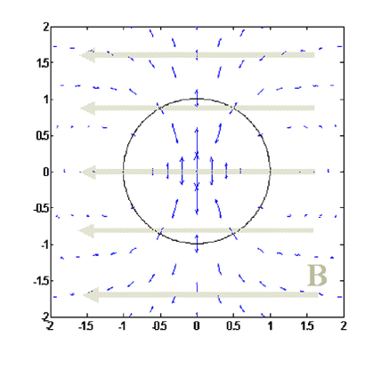
Figure 15: Polarization from a uniform magentic field (following Granot and Königl (2003)). The circle marks the and angle where the matter moves at an angle $\Gamma^{-1}$ from the observer. Note that the polarization is maximal along the line perpendicular to the uniform field but it vanished in the other direction near the $\Gamma^{-1}$ circle.

The observed stokes parameters are weighted averages of the local stokes parameters at different regions of the shell. The instantaneous polarization is calculated using the instantaneous observed flux $F_{\nu}(y,T)\propto(1+y)^{-(3+\alpha)}$, with $\alpha$ the relevant spectral index at this segment, as the weights, where $y\equiv(\Gamma\theta)^{2}$ and $T$ is the observer time. The time integrated polarization is calculated using the fluences as weights: $\int^{\infty}_{0}F_{\nu}(y,T)dT\propto(1+y)^{-(2+\alpha)}$.

The fluxes depend on how the intensity varies with the magnetic field. For $I_{\nu}\propto B^{0}$, which is relevant for fast cooling (and the prompt GRB), the time integrated stokes parameters (note that $V=0$ as the polarization is linear) and polarization are given by:

$$\frac{\left\{\begin{array}[]{c}Q\\ U\\ \end{array}\right\}}{I}=\Pi_{synch}\frac{\int_{0}^{2\pi}\int_{0}^{\infty}(1+y)^{-(2+\alpha)}\left\{\begin{array}[]{c}\cos(2\theta_{p})\\ \sin(2\theta_{p})\\ \end{array}\right\}dyd\phi}{\int_{0}^{2\pi}\int_{0}^{\infty}(1+y)^{-(2+\alpha)}dyd\phi},$$ (38)

and the relative polarization is given by

$$\Pi=\frac{\sqrt{U^{2}+Q^{2}}}{I},$$ (39)

where $\theta_{p}=\phi+\arctan(\frac{1-y}{1+y}\cot\phi)$ Granot and Königl (2003) (see also Lyutikov et al. (2003)). For $\alpha=1$ Eqs. 38-39 yield a polarization level of $\Pi/\Pi_{synch}\approx 60\%$. I.e. 60% of the maximal synchrotron polarization, or an overall polarization of $\sim 45\%$. Taking the exact values of $\alpha$ and the dependence of $I_{\nu}$ on $B$ for fast cooling and $p=2.5$ results in an overall polarization of $\sim 50\%$ Granot and Königl (2003); Nakar et al. (2003c).

It turns out that one can get a polarized emission even from random magnetic field Gruzinov and Waxman (1999) and Medvedev and Loeb (1999). This happens if the system has non spherical geometry. Consider a two dimensional random magnetic field which is in the plane of the shock and assume that the correlation length of this magnetic field is very short compared to all other length scales in the system. The Lorentz transformation induce in this case a radial polarization pattern going out from the center (where the velocity of the matter is towards the observer and the polarization vanishes). This polarization pattern is shown in Fig. 16. It is clear that a simple integration over this pattern will lead to a vanishing polarization.

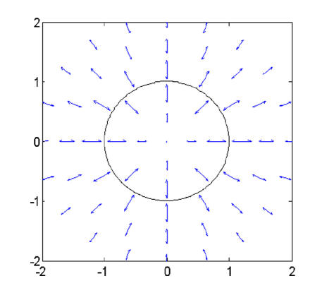
Figure 16: Polarization from a random magnetic field in the plane of the shock Nakar et al. (2003c). The solid circle marks the and angle where the matter moves at an angle $\Gamma^{-1}$ from the observer. Polarization can arise if we view a part of a jet (dashed line), or if the emission is dominated by hot spot (dashed - dotted regions) or if there is an overall gradient of the emissivity as would arise in the standard jet model.

However, a net polarization can arise in several cases if the overall symmetry is broken. Polarization will arise if (see Fig. 16):

• We observe a jet in an angle so that only a part of the jet is within an angle of $\Gamma^{-1}$.

• If the emission is nonuniform and there are stronger patches with angular size smaller than $\Gamma^{-1}$from which most of the emission arise.

• We observe a standard jet whose emission is angle dependent and this dependence is of the order of $\Gamma^{-1}$.

Gruzinov (1999); Ghisellini and Lazzati (1999); Sari (1999b); Waxman (2003) suggested that polarization can arise from a jet even if the magnetic field is random. Nakar et al. (2003c) considered a random magnetic field that remains planner in the plane of the shock (for a three dimensional random magnetic field the polarization essentially vanishes). For $I_{\nu}\propto B^{0}$ the degree of observed polarization of the emission emitted from a small region at angle $y$ is: $\Pi(y)/\Pi_{synch}=min(y,1/y)$. The overall time integrated stokes parameters are:

$$\frac{\left\{\begin{array}[]{c}Q\\ U\\ \end{array}\right\}}{I}=\Pi_{synch}\frac{\int_{0}^{2\pi}\int_{0}^{\infty}P^{\prime}_{\nu^{\prime},m}(1+y)^{-(2+\alpha)}\min(y,1/y)\left\{\begin{array}[]{c}\cos(2\phi)\\ \sin(2\phi)\\ \end{array}\right\}dyd\phi}{\int_{0}^{2\pi}\int_{0}^{\infty}P^{\prime}_{\nu^{\prime},m}(1+y)^{-(2+\alpha)}dyd\phi},$$ (40)

where $P^{\prime}_{\nu^{\prime},m}=P^{\prime}_{\nu^{\prime},m}(y,\phi)$ is the emitted power at the synchrotron frequency in the fluid rest frame. For a top-hat jet with sharp edges $P^{\prime}_{\nu^{\prime},m}$ is constant for any $y$ and $\phi$ within the jet and zero otherwise. For a structured jet $P^{\prime}_{\nu^{\prime},m}$ depends on the angle from the jet axis.

The maximal polarization is observed when one sees the edge of the jet. The probability to see the edge of a top-hat jet with sharp edges and an opening angle $\theta_{j}\Gamma\gg 1$ is negligible. On the other hand a jet with $\theta_{j}\Gamma\ll 1$ is not expected. Thus the only physical cases in which we can expect a large polarization are $1\lesssim\theta_{j}\Gamma<{\textrm{a few }}$.

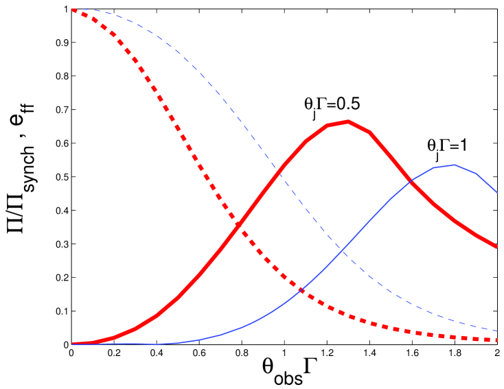
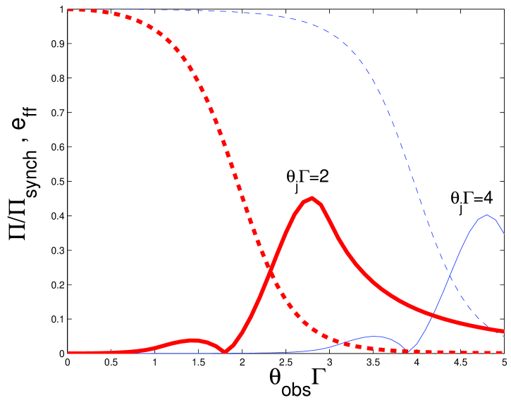
Figure 17: The time integrated polarization (solid line) and the efficiency (dashed line) as a function of $\theta_{obs}\Gamma$ for four different values of $\theta_{j}$ for a random magnetic field.

Fig. 17 depicts the time integrated polarization and the efficiency from sharp edged jets with different opening angles as a function of the angle between the jet axis and the line of sight, $\theta_{obs}$. The efficiency, $e_{ff}$ is defined to be the ratio between the observed fluence at $\theta_{obs}$ and the maximal possible observed fluence at $\theta_{obs}=0$. In all these cases the polarization is peaked above 40%, however the efficiency decrease sharply as the polarization increase. Thus the probability to see high polarization grows when $\theta_{j}$ decrease. The probability that $\theta_{obs}$ is such that the polarization is larger than $30\%$ ($\cdot\Pi_{synch}$) while $e_{ff}>0.1$ is 0.68, 0.41, 0.2 & 0.08 for $\theta_{j}\Gamma=0.5,1,2,4$ respectively. In reality this probability will be smaller, as the chance to observe a burst increases with its observed flux.

These later calculations also apply for IC emission Lazzati et al. (2003); Dar and De Rujula (2003). However, in this case the intrinsic local polarization is around 100% and hence one can reach a maximal polarization of $\sim 70$%.

Polarization could also arise if the magnetic field is uniform over random patches within a region of size $\Gamma^{-1}$. Here it is difficult, of course to estimate the total polarization without a detailed model of the structure of the jet Gruzinov and Waxman (1999).

VI THE GRB AND THE PROMPT EMISSION

I turn now to discussion of the theory of the GRB and the prompt emission. It is generally accepted that both the GRB and the afterglow arise due to dissipation of the kinetic energy of the relativistic flow. The relativistic motion can be dissipated by either external Mészáros and Rees (1992); Rees and Mészáros (1992); Katz (1994) or internal shocks Narayan et al. (1992); Paczynski and Xu (1994); Rees and Mészáros (1994). The first involve slowing down by the external medium surrounding the burst. This would be the analogue of a supernova remnant in which the ejecta is slowed down by the surrounding ISM. Like in SNRs external shocks can dissipate all the kinetic energy of the relativistic flow. On the other hand internal shocks are shocks within the flow itself. These take place when faster moving matter takes over a slower moving shell.

Sari and Piran (1997b) have shown that external shocks cannot produce variable bursts (see also Fenimore et al. (1996)). By variable I mean here, following Sari and Piran (1997b) that $\delta t\ll T$, where $T$ is the overall duration of the burst (e.g. $T_{90}$) and $\delta t$ is the duration of a typical pulse (see §II.1.2). As most GRBs are variable Sari and Piran (1997b) concluded that most GRBs are produced by internal shocks Rees and Mészáros (1994). Internal shocks can dissipate only a fraction of the kinetic energy. Therefore, they must be accompanied by external shocks that follow and dissipate the remaining energy. This leads to the internal-external shocks scenario Piran and Sari (1998). GRBs are produced by internal shocks within a relativistic flow. Subsequent external shocks between the flow and the circum-burst medium produce a smooth long lasting emission - the afterglow. Various observations (see §II.1.6) support this picture. I begin with the discussion with a comparison of internal vs. external shocks. I review then the prompt emission from internal shocks, then the prompt emission from external shocks (which includes contributions to the late part of long GRBs and the prompt optical flash). I also discuss the transition from the observations of one shock to the other.

VI.1 Internal vs. External Shocks

VI.1.1 General Considerations

Consider a “quasi” spherical relativistic emitting shell with a radius $R$, a width $\Delta$ and a Lorentz factor $\Gamma$. This can be a whole spherical shell or a spherical like section of a jet whose opening angle $\theta$ is larger than $\Gamma^{-1}$. Because of relativistic beaming an observer would observe radiation only from a region of angular size $\sim\Gamma^{-1}$. Consider now photons emitted at different points along the shock (see Fig. 18). Photons emitted by matter moving directly towards the observer (point A in Fig. 18) will arrive first. Photons emitted by matter moving at an angle $\Gamma^{-1}$ (point D in Fig. 18) would arrive after $t_{ang}=R/2c\Gamma^{2}$. This is also, $t_{R}$, the time of arrival of photons emitted by matter moving directly towards the observer but emitted at $2R$ (point C in Fig. 18). Thus, $t_{R}\approx t_{ang}$ Sari and Piran (1997b); Fenimore et al. (1996). This coincidence is the first part of the argument that rules out external shocks in variable GRBs.

Figure 18: Different time scale from a relativistic expanding shell in terms of the arrival times ($t_{i}$) of various photons: $t_{ang}=t_{D}-t_{A}$, $t_{R}=t_{C}-t_{A}$ and $t_{\Delta}=t_{B}-t_{A}$.

At a given point particles are continuously accelerated and emit radiation as long as the shell with a width $\Delta$ is crossing this point. The photons emitted at the front of this shell will reach the observer a time $t_{\Delta}=\Delta/c$ before those emitted from the rear (point B in Fig. 18). In fact photons are emitted slightly longer as it takes some time for the accelerated electrons to cool. However, for most reasonable parameters the cooling time is much shorter from the other time scales Sari et al. (1996) and I ignore it hereafter.

The emission from different angular points smoothes the signal on a time scale $t_{ang}$. If $t_{\Delta}\leq t_{ang}\approx t_{R}$ the resulting burst will be smooth with a width $t_{ang}\approx t_{R}$. The second part of this argument follows from the hydrodynamics of external shocks. I show later in §VI.3 (see also Sari and Piran (1997b)) that for external shocks $\Delta/c\leq R/c\Gamma^{2}\approx t_{R}\approx t_{ang}$ and for a spreading shell $\Delta\approx R/c\Gamma^{2}$. Therefore external shocks can produce only smooth bursts!

As we find only two time scales and as the emission is smoothed over a time scale $t_{ang}$, a necessary condition for the production of a variable light curve is that $t_{\Delta}=\Delta/c>t_{ang}$. In this case $t_{\Delta}$ would be the duration of the burst and $t_{ang}$ the variability time scale. This can be easily satisfied within internal shocks (see Fig 19). Consider an “inner engine” emitting a relativistic wind active over a time $t_{\Delta}=\Delta/c$ ($\Delta$ is the overall width of the flow in the observer frame). The source is variable on a scale $L/c$. Internal shocks will take place at $R_{s}\approx L\Gamma^{2}$. At this place the angular time and the radial time satisfy: $t_{ang}\approx t_{R}\approx L/c$. Internal shocks continue as long as the source is active, thus the overall observed duration $T=t_{\Delta}$ reflects the time that the “inner engine” is active. Note that now $t_{ang}\approx L/c<t_{\Delta}$ is trivially satisfied. The observed variability time scale in the light curve, $\delta t$, reflects the variability of the source $L/c$. While the overall duration of the burst reflects the overall duration of the activity of the “inner engine”.

Numerical simulations Kobayashi et al. (1997) have shown that not only the time scales are preserved but the source’s temporal behavior is reproduced on an almost one to one basis in the observed light curve. This can be explained now Nakar and Piran (2002a) by a simple toy model (see §VI.2.3 below).

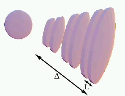
Figure 19: The internal shocks model (from Sari (1999a)) Faster. shells collide with slower ones and produce the observed $\gamma$ rays. The variability time scale is $L/c$ while the total duration of the burst is $\Delta/c$ .

VI.1.2 Caveats and Complications

Clearly the way to get around the previous argument is if $t_{ang}<t_{R}$. In this case one can identify $t_{R}$ with the duration of the burst and $t_{ang}$ as the variability time scale. The observed variability would require in this case that: $t_{ang}/t_{R}=\delta t/T$. For this the emitting regions must be smaller than $R/\Gamma$.

One can imagine an inhomogenous external medium which is clumpy on a scale $d\ll R/\Gamma$ (see Fig 20). Consider such a clump located at an angle $\theta\sim\Gamma^{-1}$ to the direction of motion of the matter towards the observer. The resulting angular time, which is the difference in arrival time between the first and the last photons emitted from this clump would be:$\sim d/c\Gamma$. Now $t_{ang}\sim{d/c\Gamma}<t_{R}$ and it seems that one can get around the argument presented before.

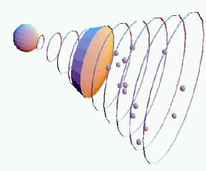
Figure 20: The clumpy ISM model (from Sari (1999a)). Note the small covering factor and the resulting “geometrical” inefficiency.

However, Sari and Piran Sari and Piran (1997b) have shown that such a configuration would be extremely inefficient. This third part of this argument rules out this caveat. The observations limit the size of the clumps to $d\approx c\Gamma\delta t$ and the location of the shock to $R\approx cT\Gamma^{2}$. The number of clumps within the observed angular cone with an opening angle $\Gamma^{-1}$ equals the number of pulses which is of the order $T/\delta t$. The covering factor of the clumps can be directly estimated in terms of the observed parameters by multiplying the number of clumps ($T/\delta t$) times their area $d^{2}=(\delta t\Gamma)^{2}$ and dividing by the cross section of the cone $(R/\Gamma)^{2}$. The resulting covering factor equals $\delta t/T\ll 1$. The efficiency of conversion of kinetic energy to $\gamma$-rays in this scenario is smaller than this covering factor which for a typical variable burst could be smaller than $10^{-2}$.

I turn now to several attempts to find a way around this result. I will not discuss here the feasibility of the suggested models (namely is it likely that the surrounding matter will be clumpy on the needed length scale Dermer and Mitman (1999), or can an inner engine eject “bullets” Heinz and Begelman (1999) with an angular width of $\sim 10^{-2}$ degrees and what keeps these bullets so small even when they are shocked and heated). I examine only the question whether the observed temporal structure can arise within these models.

VI.1.3 External Shocks on a Clumpy Medium sec:Clumpy

Dermer and Mitman (1999) claim that the simple efficiency argument of Sari and Piran (1997b) was flawed. They point out that if the direction of motion of a specific blob is almost exactly towards the observer the corresponding angular time will be of order $d^{2}/cR$ and not $d/{c\Gamma}$ used for a “generic” blob. This is narrower by a factor $d\Gamma/R$ than the angular time across the same blob that is located at a typical angle of $\Gamma^{-1}$. These special blobs would produce strong narrow peaks and will form a small region along a narrow cone with a larger covering factor. Dermer and Mitman (1999) present a numerical simulation of light curves produced by external shocks on a clumpy inhomogeneous medium with $\delta t/T\sim 10^{-2}$ and efficiency of up to $\sim 10$%.

A detailed analysis of the light curve poses, however, several problems for this model. While this result is marginal for bursts with $\delta t/T\sim 10^{-2}$ with a modulation of 50% it is insufficient for bursts with $\delta t/T\sim 10^{-3}$ or if the modulation is $\sim 100\%$. Variability on a time scale of milliseconds has been observed Nakar and Piran (2002b) in many long GRBs (namely $\delta t/T$ can be as small as $10^{-4}$.). Moreover, in this case one would expect that earlier pulses (that arise from blobs along the direction of motion) would be narrower than latter pulses. This is not seen in the observed bursts Ramirez-Ruiz and Fenimore (2000).

Finally the arrival time of individual pulses depends on the position of the emitting clumps relative to the observers. Two following pulses would arise from two different clumps that are rather distant from each other. There is no reason why the pulses and intervals should be correlated in any way. Recall (§II.1.2) that the duration of a pulse and the subsequent interval are correlated Nakar and Piran (2002c).

VI.1.4 The Shot-Gun Model

Heinz and Begelman (1999) suggested that the “inner engine” operates as a shot-gun emitting multiple narrow bullets with an angular size much smaller than $\Gamma^{-1}$ (see Fig 21). These bullets do not spread while propagating and they are slowed down rapidly by an external shock with a very dense circumburst matter. The pulses width is given by $t_{ang}$ or by the slowing down time. The duration of the burst is determined by the time that the “inner engine” emits the bullets.

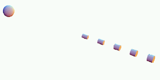
Figure 21: The shot-gun model (from Sari (1999a)). The inner engine emits narrow “bullets” that collide with the ISM.

This model can produce the observed variability and like in the internal shocks model the observed light curve represents also here the temporal activity of the source. However, in this model the width of the pulses is determined by the angular time or the hydrodynamic time or the cooling time of the shocked material. On the other hand the intervals between the pulses depend only on the activity of the inner engine. Again, there is no reason why the two distributions will be similar and why there should be a correlation between them (see §II.1.2 and Nakar and Piran (2002c)).

VI.1.5 Relativistic Turbulence

An interesting alternative to shocks as a way to dissipate kinetic energy is within plasma turbulence Smolsky and Usov (1996, 2000); Lyutikov and Blandford (2002, 2003). It has been suggested that in this case the kinetic energy of the shock is dissipated downstream to a combination of macroscopic (relativistic) random motion of plasma blobs with a Lorentz factor $\Gamma_{b}$. Within these blobs the particles have also a (relativistic) random velocity with a Lorentz factor $\Gamma_{p}$, such that: $\Gamma_{s}\approx\Gamma_{b}\Gamma_{p}$.

Relativistic turbulence may be the only way to produce variability in a situation that the matter is slowed down by the external medium and not by internal interaction. I stress that in this case the process is not described by regular shocks and hence some of the previous arguments do not hold. Two crucial open questions are i) Whether one can produce the observed correlations between pulses and intervals. ii) Why there is no spreading of pulses at later times, as would be expected if the emitting region is slowing down and increasing its radius.

VI.2 Internal Shocks

VI.2.1 Hydrodynamics of Internal Shocks

Internal shocks take place when a faster shell catches a slower one, namely at:

$$R_{int}\approx c\delta t\Gamma^{2}=3\times 10^{14}{\rm cm}\Gamma_{100}^{2}\tilde{\delta}t$$ (41)

where $\Gamma_{100}$ is the typical Lorentz factor in units of $10^{2}$ and $\tilde{\delta}t$ is the time difference between the emission of the two shells. I show later that $\tilde{\delta}t$ defined here is roughly equal to the observed fluctuations in the light curve of the burst $\delta t$. Clearly $R_{int}<R_{ext}$ must hold otherwise internal shocks won’t take place. $R_{ext}$ is defined as the location of efficient extraction of energy by external shocks (see §VI.3). If follows from the discussion in §VI.3 that the condition $R_{int}<R_{ext}$ implies:

$$\delta\Gamma^{2}<{\rm max}({l\over\Gamma^{2/3}},l^{3/4}\Delta^{1/4})$$ (42)

where $l$ is defined by Eq. 57 and it is typically of the order of $10^{18}$cm, while $\Delta$ is the width of the shell and it is of order $10^{12}$cm. Both conditions set upper limits on $\Gamma$ (of the order of a few thousands) for internal shocks. If the initial Lorentz factor is too large then internal shocks will take place at large radii and external shocks will take place before the internal shocks could take place. It is possible that this fact plays an important role in limiting the relevant Lorentz factors and hence the range of variability of $E_{p}$, the peak energy observed in GRBs.

Internal shocks are characterized by a comparable Lorentz factor of order of a few ($1<\Gamma<10$) reflecting the relative motion of the shells and by comparable densities $n$ in both shells. In this case, for an adiabatic index (4/3), the Loretz factor of the shocked region $\hat{\Gamma}$ satisfies:

$$\hat{\Gamma}=\sqrt{(\Gamma^{2}+1)/2}\ \ .$$ (43)

The shocked density $\hat{n}$ and energy $\hat{e}$ are:

$${\hat{n}}=(4{\hat{\Gamma}}+3)n\approx 4{\hat{\Gamma}}n\ \ ;\ \ {\hat{e}}={\hat{\Gamma}}{\hat{n}}m_{p}c^{2}\ .$$ (44)

Both shocks are mildly relativistic and their strength depends on the relative Lorentz factors of the two shells.

VI.2.2 The Efficiency of Internal Shocks

Consider collision between two shells with masses $m_{r}$ and $m_{s}$ that are moving at different relativistic velocities: $\Gamma_{r}\gtrsim\Gamma_{s}\gg 1$. The resulting bulk Lorentz factor, $\Gamma_{m}$ in an elastic collision is:

$$\Gamma_{m}\simeq\sqrt{\frac{m_{r}\Gamma_{r}+m_{s}\Gamma_{s}}{m_{r}/\Gamma_{r}+m_{s}/\Gamma_{s}}}.$$ (45)

The internal energy, ${\cal E}_{int}$, in the local frame and $E_{int}$, in the frame of an external observer, of the merged shell: $E_{int}=\Gamma_{m}{\cal E}_{int}$, is the difference of the kinetic energies before and after the collision:

$$E_{int}=m_{r}c^{2}(\Gamma_{r}-\Gamma_{m})+m_{s}c^{2}(\Gamma_{s}-\Gamma_{m}).$$ (46)

The conversion efficiency of kinetic energy into internal energy is Kobayashi et al. (1997):

$$\epsilon=1-{(m_{r}+m_{s})\Gamma_{m}\over(m_{r}\Gamma_{r}+m_{s}\Gamma_{s})}.$$ (47)

As can be expected a conversion of a significant fraction of the initial kinetic energy to internal energy requires that the difference in velocities between the shells will be significant: $\Gamma_{r}\gg\Gamma_{s}$ and that the two masses will be comparable $m_{r}\approx m_{s}$ Kobayashi et al. (1997); Daigne and Mochkovitch (1998).

Beloborodov (2000) considered internal shocks between shells with a lognormal distribution of $(\Gamma-1)/(\Gamma_{0}-1)$, where $\Gamma_{0}$ is the average Lorentz factor. The dimensionless parameter, $A$, measures the width of the distribution. He shows that the efficiency increases and reached unity when $A$ is of order unity, that is typical fluctuation in $\Gamma$ are by a factor of 10 compared to the average. Similarly numerical simulations of Guetta et al. (2001a) show that a significant fraction of the wind kinetic energy, on the order of 20%, can be converted to radiation, provided the distribution of Lorentz factors within the wind has a large variance and the minimum Lorentz factor is greater than $\approx 10^{2.5}L^{2/9}_{52}$, where $L_{52}$ is the (isotropic) wind luminosity in units of $10^{52}$ergs/sec.

Another problem that involves the efficiency of GRBs is that not all the internal energy generated is emitted. This depends further on $\epsilon_{e}$, the fraction of energy given to the electron. If this fraction is small and if there is no strong coupling between the electrons and the protons the thermal energy of the shocked particles (which is stored in this case mostly in the protons) will not be radiated away. Instead it will be converted again to kinetic energy by adiabatic cooling. Kobayashi and Sari (2001) consider a more elaborated model in which colliding shells that do not emit all their internal energy are reflected from each other, causing subsequent collisions and thereby allowing more energy to be emitted. In this case more energy is eventually emitted than what would have been emitted if we considered only the first collision. They obtain about 60% overall efficiency even if the fraction of energy that goes to electrons is small $\epsilon_{e}=0.1$. This is provided that the shells’ Lorentz factor varies between 10 and 10⁴.

VI.2.3 Light Curves from Internal Shocks

Both the similarity between the pulse width and the pulse separation distribution and the correlation between intervals and the subsequent pulses Nakar and Piran (2002c); Quilligan et al. (2002) arise naturally within the internal shocks model Nakar and Piran (2002a). In this model both the pulse duration and the separation between the pulses are determined by the same parameter - the interval between the emitted shells. I outline here the main argument (see Nakar and Piran (2002a) for details). Consider two shells with a separation $L$. The Lorentz factor of the slower outer shell is $\Gamma_{S}=\Gamma$ and of the Lorentz factor inner faster shell is $\Gamma_{F}=a\Gamma$ ($a>2$ for an efficient collision). Both are measured in the observer frame. The shells are ejected at $t_{1}$ and $t_{2}\approx t_{1}+L/c$. The collision takes place at a radius $R_{s}\approx 2\Gamma^{2}L$ (Note that $R_{s}$ does not depend on $\Gamma_{2}$). The emitted photons from the collision will reach the observer at time (omitting the photons flight time, and assuming transparent shells):

$$t_{o}\approx t_{1}+R_{s}/(2c\Gamma^{2})\approx t_{1}+L/c\approx t_{2}\ .$$ (48)

The photons from this pulse are observed almost simultaneously with a (hypothetical) photon that was emitted from the “inner engine” together with the second shell (at $t_{2}$). This explains why various numerical simulations Kobayashi et al. (1997); Daigne and Mochkovitch (1998); Panaitescu et al. (1999) find that for internal shocks the observed light curve replicates the temporal activity of the source.

In order to determine the time between the bursts we should consider multiple collisions. It turns out that there are just three types of collisions, (i), (ii) and (iii), that characterize the system and all combinations of multiple collisions can be divided to these three types. Consider four shells emitted at times $t_{i}$ ($i=1,2,3,4$) with a separation of the order of $L$ between them. In type (i) there are two collisions - between the first and the second shells and between the third and the fourth shells. The first collision will be observed at $t_{2}$ while the second one will be observed at $t_{4}$. Therefore, $\Delta t\approx t_{4}-t_{2}\approx 2L/c$. A different collision scenario (ii) occurs if the second and the first shells collide, and afterward the third shell takes over and collide with them (the forth shell does not play any roll in this case). The first collision will be observed at $t_{2}$ while the second one will be observed at $t_{3}$. Therefore, $\Delta t\approx t_{3}-t_{2}\approx L/c.$ Numerical simulations Nakar and Piran (2002a) show that more then 80% of the efficient collisions follows one of these two scenarios ((i) or (ii)). Therefore one can estimate:

$$\Delta t\approx L/c\ .$$ (49)

Note that this result is independent of the shells’ masses.

A third type of a multiple collision (iii) arises if the third shell collides first with the second shell. Then the merged shell will collide with the first one (again the fourth shell does not participate in this scenario). In this case the two pulses merge and will arrive almost simultaneously, at the same time with a (hypothetical) photon that would have been emitted from the inner engine simultaneously with the third (fastest) shell. $t\sim t_{3}$. Only a 20% fraction exhibits this type of collision.

The pulse width is determined by the angular time (ignoring the cooling time): $\delta t=R_{s}/(2c\Gamma^{2}_{s})$ where $\Gamma_{s}$ is the Lorentz factor of the shocked emitting region. If the shells have an equal mass ($m_{1}=m_{2}$) then $\Gamma_{s}=\sqrt{a}\Gamma$ while if they have equal energy ($m_{1}=am_{2}$) then $\Gamma_{s}\approx\Gamma$. Therefore:

$$\delta t\approx\left\{\begin{array}[]{r@{\quad\quad}l}R_{s}/2a\Gamma^{2}c\approx L/ac&\rm{equal\ mass},\\ R_{s}/2\Gamma^{2}c\approx L/c&\rm{equal\ energy}.\end{array}\right.$$ (50)

The ratio of the Lorentz factors $a$, determines the collision’s efficiency. For efficient collision the variations in the shells Lorentz factor (and therefore $a$) must be large.

It follows from Eqs. 49 and 50 that for equal energy shells the $\Delta t$-$\delta t$ similarity and correlation arises naturally from the reflection of the shells initial separation in both variables. However, for equal mass shells $\delta t$ is shorter by a factor of $a$ than $\Delta t$. This shortens the pulses relative to the intervals. Additionally, the large variance of $a$ would wipe off the $\Delta t$-$\delta t$ correlation. This suggests that equal energy shells are more likely to produce the observed light curves.

VI.3 External Shocks

VI.3.1 Hydrodynamics

Consider the situation when a cold relativistic shell (whose internal energy is negligible compared to the rest mass) moves into the cold ISM. Generally, two shocks form: an outgoing shock that propagates into the ISM or into the external shell, and a reverse shock that propagates into the inner shell, with a contact discontinuity between the shocked material (see Fig. 22).

There dual shocks system is divided to four distinct regions (see Fig. 22): the ambient matter at rest (denoted by the subscript 1), the shocked ambient matter which has passed through the forward shock (subscript 2 or f), the shocked shell material which has passed through the reverse shock (subscript 3 or r), and the unshocked material of the shell (subscript 4). The nature of the emitted radiation and the efficiency of the cooling processes depend on the conditions in the shocked regions 2 and 3. Both regions have the same energy density $e$. The particle densities $n_{2}$ and $n_{3}$ are, however, different and hence the effective “temperatures,” i.e. the mean Lorentz factors of the random motions of the shocked protons and electrons, are different.

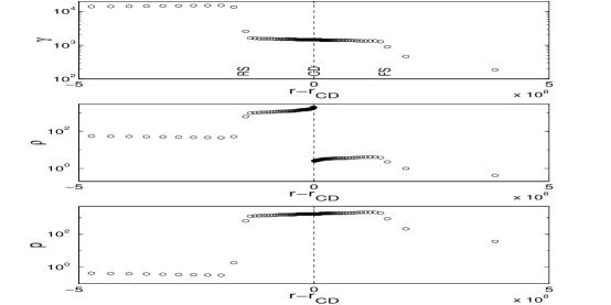
Figure 22: The Lorentz factor $\Gamma$, the density $\rho$ and the pressure $p$ in the shocks. There are four regions: the ISM (region 1), the shocked ISM (region 2), the shocked shell (region 3) and the un-shocked shell (region 4), which are separated by the forward shock (FS), the contact discontinuity (CD) and the reverse shock (RS). From Kobayashi et al. (1999).

Two quantities determine the shocks’ structure: $\Gamma$, the Lorentz factor of the motion of the inner expanding matter (denoted 4) relative to the outer matter (the ISM or the outer shell in the case of internal collisions - denoted 1) , and the ratio between the particle number densities in these regions, $n_{4}/n_{1}$. Initially the density contrast between the spherically expanding shell and the ISM is large. Specifically $n_{4}/n_{1}>\Gamma^{2}$. This happens during the early phase of an external shock when the shell is small and dense. This configuration is denoted “Newtonian” because the reverse shock is non-relativistic at most (or mildly relativistic). In this case all the energy conversion takes place in the forward shock. Only a negligible fraction of the energy is converted to thermal energy in the reverse shock if it is Newtonian Sari and Piran (1995). Let $\Gamma_{2}$ be the Lorentz factor of the motion of the shocked fluid relative to the rest frame of the fluid at 1 and let $\bar{\Gamma}_{3}$ be the Lorentz factor of the motion of this fluid relative to the rest frame of the relativistic shell (4):

$$\Gamma_{2}\approx\Gamma\ \ \ ;\ \ \ \bar{\Gamma}_{3}\approx 1.$$ (51)

The particle and energy densities $(n,e)$ in the shocked regions satisfy:

$$n_{2}\approx 4\Gamma n_{1},\ \ ;\ \ e\equiv e_{2}=4\Gamma^{2}n_{1}m_{p}c^{2}\ \ ;\ \ n_{3}=7n_{4},\ \ ;\ \ e_{3}=e.$$ (52)

Later, the shell expands and the density ratio decreases (like $R^{-2}$ if the width of the shell is constant and like $R^{-3}$ if the shell is spreading) and $n_{4}/n_{1}<\Gamma^{2}$ (but $n_{4}/n_{1}>1$). In this case both the forward and the reverse shocks are relativistic. The shock equations between regions 1 and 2 combined with the contact discontinuity between 3 and 2 yield Blandford and McKee (1976, 1977); Piran (1994):

$$\Gamma_{2}=(n_{4}/n_{1})^{1/4}\Gamma^{1/2}/\sqrt{2}\ \ ;\ \ n_{2}=4\Gamma_{2}n_{1}\ \ ;\ \ e\equiv e_{2}=4\Gamma^{2}_{2}n_{1}m_{p}c^{2},$$ (53)

Similar relations hold for the reverse shock:

$$\bar{\Gamma}_{3}=(n_{4}/n_{1})^{-1/4}\Gamma^{1/2}/\sqrt{2}\ \ ;\ \ n_{3}=4\bar{\Gamma}_{3}n_{4}.$$ (54)

Additinally,

$$e_{3}=e\ \ ;\ \ \bar{\Gamma}_{3}\cong(\Gamma/\Gamma_{2}+\Gamma_{2}/\Gamma)/2\ ,$$ (55)

which follow from the equality of pressures and velocity on the contact discontinuity. Comparable amounts of energy are converted to thermal energy in both shocks when both shocks are relativistic.

The interaction between a relativistic flow and an external medium depends on the Sedov length that is defined generally as:

$$E=m_{p}c^{2}\int_{0}^{l}4\pi n(r)r^{2}dr\ .$$ (56)

The rest mass energy within the Sedov sphere equals the energy of the explosion. For a homogeneous ISM:

$$l\equiv({E\over(4\pi/3)n_{ism}m_{p}c^{2}})^{1/3}\approx 10^{18}{\rm cm}E_{52}^{1/3}n_{1}^{1/3}\ .$$ (57)

Note that in this section $E$ stands for the isotropic equivalent energy. Because of the very large Lorentz factor angular structure on a scale larger than $\Gamma^{-1}$ does not influence the evolution of the system and it behaves as if it is a part of a spherical system. A second length scale that appears in the problem is $\Delta$, the width of the relativistic shell in the observer’s rest frame.

Initially the reverse shocks is Newtonian and only a negligible amount of energy is extracted from the shell. At this stage the whole shell acts “together”. Half of the shell’s kinetic energy is converted to thermal energy when the collected external mass is $M/\Gamma$, where $M$ is the shell’s mass Rees and Mészáros (1992); Katz (1994). This takes place at a distance:

$$R_{\Gamma}={l\over\Gamma^{2/3}}=\bigg{(}{E\over n_{ism}m_{p}c^{2}\Gamma^{2}}\bigg{)}^{1/3}=5.4\times 10^{16}~{}{\rm cm}~{}E_{52}^{1/3}n_{1}^{-1/3}\Gamma_{100}^{-2/3},$$ (58)

where $E_{52}$ is the equivalent isotropic energy in $10^{52}$ergs, $n_{1}=n_{ism}/1~{}{\rm particle/cm}^{3}$.

However, the reverse shock might become relativistic before $R_{\Gamma}$. Now energy extraction from the shell is efficient and one passage of the reverse shock through the shell is sufficient for complete conversion of the shell’s energy to thermal energy. The energy of the shell will be extracted during a single passage of the reverse shock across the shell. Using the expression for the velocity of the reverse shock into the shell (Eq. 54) one finds that the reverse shock reaches the inner edge of the shell at $R_{\Delta}$ Sari and Piran (1995):

$$R_{\Delta}=l^{3/4}\Delta^{1/4}\approx 10^{15}{\rm cm}l_{18}^{3/4}\Delta_{12}^{1/4}\ .$$ (59)

The reverse shock becomes relativistic at $R_{N}$, where $n_{4}/n_{1}=\Gamma^{2}$:

$$R_{N}=l^{3/2}/\Delta^{1/2}\Gamma^{2}$$ (60)

Clearly, if $R_{N}>R_{\Gamma}$ then the energy of the shell is dissipated while the shocks are still “Newtonain”. If $R_{N}<R_{\Gamma}$ the reverse shock becomes relativistic. In this case $R_{\Gamma}$ looses its meaning as the radius where the energy is dissipated. The energy of the shell is dissipated in this “relativistic” case at $r_{\Delta}$. The question which of the two conditions is relevant depends on the parameter $\xi$ Sari and Piran (1995):

$$\xi\equiv(l/\Delta)^{1/2}\Gamma^{-4/3}=2(l_{18}/\Delta_{12})^{1/2}\Gamma_{100}^{-4/3}.$$ (61)

I have used a canonical value for $\Delta$ as $10^{12}$cm. It will be shown later that within the internal-external scenario $\Delta/c$ corresponds to the duration of the bursts and $10^{12}$cm corresponds to a typical burst of $30$sec.

Using $\xi$ one can express the different radii as:

$$R_{int}/\zeta=R_{\Delta}/\xi^{3/2}=R_{\gamma}\xi^{2}=R_{N}/\xi^{3}\ .$$ (62)

For completeness I have added to this equation $R_{Int}$, where internal shocks take place (see Eq. 41). The dimensionless quantity $\zeta$ : $\zeta\equiv\delta/\Delta$. Thus:

$$\cases{R_{\Delta}<{\bf R_{\Gamma}}<R_{N}&$\xi>1$ { (Newtonian~{}reverse~{}shock)}\cr R_{N}<R_{\Gamma}<{\bf R_{\Delta}}&$\xi<1$ { (Relativistic~{}reverse~{}shock)}.}$$ (63)

I have marked in bold face the location where the effective energy extraction does take place. With typical values for $l$, $\Delta$ and $\Gamma$ $\xi$ is around unity. The radius where energy extraction takes place is marked in bold face!

Expanding shell: A physical shell is expected to expand during as it propagates with $\Delta=\Delta_{0}+R\Gamma^{2}$ Piran et al. (1993). This will lead to a monotoneously decreasing $\xi$. As the value of $R_{\Gamma}$ is independent of $\Delta$ it does not vary. However, $R_{\Delta}$ and $R_{N}$ decrease from their initial values. If $\Delta_{0}<R_{\Gamma}\Gamma^{2}$ (corresponding to $\xi_{0}>1$) then $\xi=1$ at $R_{\Delta}=R_{\Gamma}=R_{N}$ and all three radii coincide. Given the fact that with typical parameters $\xi$ is of order unity this seems to be the “typical” case. The reverse shocks becomes mildly relativistic just when the energy extraction becomes efficient. However, if $\xi_{0}\ll 1$ then the shell won’t expand enough and still there will be a relativistic reverse shock operating at $R_{\Delta}$. It is useful to note that in this case the effective energy extraction takes place at $R_{\Delta}$ for all initial values of $\xi_{0}$. In the following I denote by $\tilde{\xi}$ the value of $\xi$ at $R_{\Delta}$: $\tilde{\xi}\approx\xi_{0}$ if $\xi_{0}<1$ and otherwise $\tilde{\xi}\approx 1$.

Overall the external shocks take place at:

$$R_{ext}=\cases{{\rm max}({l/\Gamma^{2/3}},l^{3/4}\Delta^{1/4}),&Non spreading shell,\cr l/\Gamma^{2/3}\approx l^{3/4}\Delta^{1/4}\approx 5\times 10^{16}{\rm cm}E_{52}^{1/3}n_{1}^{1/3}\Gamma^{-2/3}_{100},&Spreading shell.\cr}$$ (64)

Usually I will use the second relation (the spreading shell one) in the following discussion. Note that in the case of non spreading shell one uses the maximum of the two possible radii. For example in the Newtonian case where the extraction is at $l/\Gamma^{2/3}$ the shocks pass the shall many times and hence $l/Gamma^{2/3}>l^{3/4}\Delta^{1/4}$.

VI.3.2 Synchrotron Spectrum from External Shocks

The bulk of the kinetic energy of the shell is converted to thermal energy via the two shocks at around the time the shell has expanded to the radius $R_{\Delta}$ (this would be the case in either a thick shell with $\xi<1$ or with an expanding shell that begins with $\xi_{0}>1$ but reaches $\xi\approx 1$ due to expansion of the shell around the time when $R_{\Gamma}=R_{\Delta}$ and efficient dissipation takes place . At this radius, the conditions at the forward shock are:

$$\Gamma_{2}=\Gamma\xi^{3/4},\ \ \ n_{2}=4\Gamma_{2}n_{1},\ \ \ e_{2}=4\Gamma_{2}^{2}n_{1}m_{p}c^{2},$$ (65)

while at the reverse shock:

$$\bar{\Gamma}_{3}=\xi^{-3/4},\ \ \ \Gamma_{3}=\Gamma\xi^{3/4},\ \ \ n_{3}=4\xi^{9/4}\Gamma^{2}n_{1},\ \ \ e_{3}=e_{2}.$$ (66)

Substitution of $\Gamma_{sh}=\Gamma_{2}=\Gamma\xi^{3/4}$ in Eq. V.1 yields, for the equipartition magnetic field:

$$B=\sqrt{32\pi}c\epsilon_{B}^{1/2}\Gamma\xi^{3/4}m_{p}^{1/2}n_{1}^{1/2}=(40~{}{\rm G})~{}\epsilon_{B}^{1/2}\xi^{3/4}{\Gamma_{100}}n_{1}^{1/2}.$$ (67)

If the magnetic field in region 2 behind the forward shock is obtained purely by shock compression of the ISM field, the field would be very weak, with $\epsilon_{B}\ll 1$. Such low fields are incompatible with observations of GRBs. I consider, therefore, the possibility that there may be some kind of a turbulent instability which brings the magnetic field to approximate equipartition Silva et al. (2003); Frederiksen et al. (2003). In the case of the reverse shock, i.e. in region 3, magnetic fields of considerable strength might be present in the pre-shock shell material if the original exploding fireball was magnetic. The exact nature of magnetic field evolution during fireball expansion depends on several assumptions. Thompson (1994) found that the magnetic field will remain in equipartition if it started off originally in equipartition. Mészáros, Laguna & Rees Meszaros et al. (1993) on the other hand, estimated that if the magnetic field was initially in equipartition then it would be below equipartition by a factor of $10^{-5}$ by the time the shell expands to $R_{\Delta}$. It is uncertain which, if either one, of the estimates is right. As in the forward shock, an instability could boost the field back to equipartition. Thus, while both shocks may have $\epsilon_{B}\ll 1$ with pure flux freezing, both could achieve $\epsilon_{B}\rightarrow 1$ in the presence of instabilities. In principle, $\epsilon_{B}$ could be different for the two shocks. For simplicity I will consider the same value in the following discussions.

Following the discussion in §V.2, I assume that in both regions 2 and 3 the electrons have a power law distribution with a minimal Lorentz factor $\gamma_{e,min}$ given by Eq. 21 with the corresponding Lorentz factors for the forward and the reverse shocks.

Forward shock: The typical energy of synchrotron photons as well as the synchrotron cooling time depend on the Lorentz factor $\gamma_{e}$ of the relativistic electrons under consideration and on the strength of the magnetic field. Using Eq. 21 for $\gamma_{e,min}$ and Eq. 15 for the characteristic synchrotron energy for the forward shock:

$$(h\nu_{syn})_{obs|\gamma_{e,min}}=160~{}{\rm keV}~{}\epsilon_{B}^{1/2}\epsilon_{e}^{2}\Gamma_{2,100}^{4}n_{1}^{1/2}=0.5~{}{\rm keV}~{}(\epsilon_{B}/0.1)^{1/2}(\epsilon_{e}/0.1)^{2}\tilde{\xi}_{0}^{3}\Gamma_{100}^{4}n_{1}^{1/2},$$ (68)

and

$$t_{syn|\gamma_{e,min}}=0.085~{}{\rm sec}~{}\epsilon_{B}^{-1}\epsilon_{e}^{-1}\Gamma_{2,100}^{-4}n_{1}^{-1}=0.085~{}{\rm sec}~{}\epsilon_{B}^{-1}\epsilon_{e}^{-1}\tilde{\xi}^{-3}\Gamma_{100}^{-4}n_{1}^{-1}$$ (69)

The characteristic frequency and the corresponding cooling time for the “typical” electron are larger and shorter by a factor of $[(p-2)/(p-1)]^{2}$, correspondingly.

The electrons at the forward shock are fast cooling and w the typical cooling frequency is Sari and Piran (1999c):

$$\nu_{c}=6keV(\epsilon_{B}/0.1)^{-3/2}(\Gamma_{2}/100)^{-4}n_{1}^{-3/2}t_{s}^{-2}\ ,$$ (70)

where $t_{s}$ is the time in seconds. The photons from the early forward shock are in the low $\gamma$-rays to X-ray range, but this depends strongly on the various parameters (note the strong $\Gamma_{2}^{4}$ dependence in equation 68). For this set of canonical parameters $\nu_{m}<\nu_{c}$. However, the ratio of these two frequencies depends on $\Gamma^{8}$! For $\Gamma$ slightly larger then 100 the inequality will reverse and the system will be in the fast cooling regime.

Reverse Shock: The Lorentz factor of the reverse shock, $\bar{\Gamma}_{3}$ is smaller by a factor of $\xi^{3/2}\Gamma$ than the Lorentz factor of the forward shock $\Gamma_{2}$. Similarly the Lorentz factor of a “typical electron” in the reverse shock is lower by a factor $\xi^{3/2}\Gamma$. Therefore the observed energy is lower by a factor $\xi^{3}\Gamma^{2}$. The typical synchrotron frequency of the reverse shock is

$$\nu_{m|reverse~{}shock}=1.3\times 10^{13}{\rm Hz}~{}(\epsilon_{B}/0.1)^{1/2}(\epsilon_{e}/0.1)^{2}\Gamma_{100}^{2}\ .$$ (71)

This is in the IR regions but note again the strong dependence on the Lorentz factor and on $\epsilon_{e}$, which could easily bring this frequency up to the optical regime. The cooling frequency in the reverse shock region is the same as the cooling frequency of the forward shock (if both regions have the same $\epsilon_{B}$) Sari and Piran (1999c) hence:

$$\nu_{c|reverse~{}shock}=8\times 10^{18}{\rm Hz}(\epsilon_{B}/0.1)^{-3/2}(\Gamma_{2}/{100})^{-4}n_{1}^{-3/2}t_{s}^{-2}=$$

$$8.8\times 10^{15}{\rm Hz}(\epsilon_{B}/0.1)^{-3/2}E_{52}^{-1/2}n_{1}^{-1}t_{s}^{-1/2}\ .$$ (72)

In the forward shock $\nu_{m}$ is comparable or larger than $\nu_{c}$. In the reverse shock $\nu_{m}<\nu_{c}$ and it is usually in the slow cooling regime. The reverse shocks exists for a short time until it reaches the back of the relativistic shell. Then it turns into a rarefraction wave that propagates forwards. After some back and forth bounces of these wave all the matter behind the forward shock organizes itself in the form of the Blandford-McKee self similar solution discussed latter in §VII.1. This above estimates suggest Mészáros and Rees (1997a); Sari and Piran (1999a, b, c) that during the short phase in which the reverse shock exists it should produce a powerful optical flash. This flash should coincide with the late part of the GRB. Kobayashi (2000) calculates the light curves and typical frequencies of the reverse shock for a variety of conditions.

VI.4 The Transition from Internal Shocks to External Shocks

The internal shocks take place at a distance $R_{int}\sim c\delta t\Gamma^{2}\sim(\delta t/0.3sec)\Gamma_{2}^{2}10^{14}$cm. These shocks last as long as the inner engine is active. The typical observed time scale for this activity $\sim 50$sec (for long bursts) and $\sim 0.5$sec (for short ones). External shocks begin at $R_{ext}\sim 10^{16}$cm. If $R_{ext}/\Gamma^{2}\leq T=\Delta/c$, namely if the burst is long, the afterglows begins while internal shocks are still going on and the initial part of the afterglow overlaps the late part of the GRB Sari (1997). At the early time the afterglow emission (from the forward shock) peaks in the high X-rays contributing also to the observed $\gamma$-ray flux. One can expect, therefore, a transition within the GRB from hard (pure GRB) to softer and smoother (GRB and afterglow) signal. Some observational evidence for this transition was presented in §II.1.6.

VI.5 Prompt Polarization

In §II.1.4 I discussed the detection of very high linear polarization from GRB 021206 Coburn and Boggs (2003). While the data analysis is uncertain several papers claimed that this detection has strong implications. First Coburn and Boggs (2003) suggest that this polarization indicates that the emission mechanism is synchrotron. Lyutikov et al. (2003) and Granot (2003) suggest further that it implies uniform magnetic fields within the emitting regions and the first even conclude that this implies that the relativistic flow is Poynting flux dominated and that the dissipation is in the form of external plasma instability. Waxman (2003) and Nakar et al. (2003c) show however that: (i) Random magnetic field in shock’s plane could produce almost as high polarization as a uniform field (provided that the emitting jet is narrow and one is looking along the edge of the jet). (ii) Even if the magnetic field is uniform the flow does not have to be Poynting flux dominated. They also stress that while in the uniform field case we expect high polarization in almost every burst in the random field one we can expect high polarization only in very few bursts. The different time dependence of the polarization Nakar et al. (2003c) could also enable us to distinguish between the two possibilities.

Lazzati et al. (2003) and Dar and De Rujula (2003) suggest that this polarization implies IC (which can have in principle higher intrinsic polarization). This shows that even the simplest conclusion (that the polarization confirms synchrotron as the emission mechanism) is uncertain. My overall conclusion is that without further data on other bursts (which is, unfortunately, quite unlikely in the nearby future) not much can be learnt from this tentative detection.

VII THE AFTERGLOW

It is generally accepted that the afterglow is produced when the relativistic ejecta is slowed down by the surrounding matter Mészáros and Rees (1997a). The afterglow begins at $R_{ext}$ where most of the energy of the ejecta is transferred to the shocked external medium. For a long burst this takes place while the burst is still going on (see Sari (1997) and §VI.4). Initially the process might be radiative, namely a significant fraction of the kinetic energy is dissipated and the radiation process effects the hydrodynamics of the shock. I discuss this phase in §VII.3. Later the radiation processes become less efficient and an adiabatic phase begins during which the radiation losses are minor and do not influence the hydrodynamics. The hydrodynamic evolution at this stage is adiabatic. If the ejecta is in the form of a jet with an opening angle $\theta$ then a jet transition will take place when $\Gamma$ reaches $\theta^{-1}$. A transition into the Newtonian regime takes place when $\Gamma-1\approx 0.5$. I begin the discussion of the afterglow with the hydrodynamics of the adiabatic phase and with the resulting synchrotron light curve. I continue with a discussion of the possible early radiative evolution. Then I turn to the jet break and to the Newtonian transition. I continue with various complications and variations on these themes.

VII.1 Relativistic Blast Waves and the Blandford-McKee solution

The theory of relativistic blast waves has been worked out in a classical paper by Blandford & McKee (BM) already in 1976. The BM model is a self-similar spherical solution describing an adiabatic ultra relativistic blast wave in the limit $\Gamma\gg 1$. This solution is the relativistic analogue of the well known Newtonian Sedov-Taylor solution. Blandford and McKee also describe in the same paper a generalization for varying ambient mass density, $\rho=\rho_{0}(R/R_{0})^{-k}$, $R$ being the distance from the center. The latter case would be particularly relevant for $k=2$, as expected in the case of wind from a progenitor, prior to the GRB explosion.

The BM solution describes a narrow shell of width $\sim R/\Gamma^{2}$, in which the shocked material is concentrated. For simplicity I approximate the solution with a thin homogenous shell. Then the adiabatic energy conservation yields:

$$E={\Omega\over 3-k}(\rho_{0}R_{0}^{k})R^{3-k}\Gamma^{2}c^{2}\ ,$$ (73)

where $E$ is the energy of the blast wave and $\Omega$ is the solid angle of the afterglow. For a full sphere $\Omega=4\pi$, but it can be smaller if the expansion is conical with an opening angle $\theta$: $\Omega=4\pi(1-cos\theta)\approx 2\pi\theta^{2}$ (assuming a double sided jet). This expression can be simplified using a generalized Sedov scale:

$$l=\left[(3-k)E/\rho_{0}R_{0}^{k}c^{2}\right]^{1/(3-k)}.$$ (74)

If $\Omega$ does not change with time then the blast wave collects ambient rest mass that equals its initial energy at $R=l$.If we take into account sideway expansion (after the jet break) we find that $\Gamma\approx 1$ and the blast wave becomes Newtonian at:

$$R=l(\Omega/4\pi)^{1/(3-k)}.$$ (75)

Using the approximate (the numerical factor in this equation assumes that the shell is moving at a constant velocity) time - radius relation Eq. 7 one can invert Eq. 73 (using the definition of $l$ , Eq. 74) and obtain $R$ and $\Gamma$ as a function of time:

$$R = [{2l^{3-k}\over\Omega}]^{1/(4-k)}t^{1/(4-k)}$$ (76)

$$\Gamma = [{l^{3-k}\over 2^{3-k}\Omega}]^{1/2(4-k)}t^{-(3-k)/2(4-k)}$$

The time in these expressions is the observer time - namely the time that photons emitted at $R$ arrive to the observer (relative to the time that photons emitted at $R=0$). For spherical (or spherical like) evolution $\Omega$ in these expressions is a constant. In general it is possible that $\Omega$ varies with $R$ or with $\Gamma$ (as is the case in a sideways expansion of a jet). This will produce, of course, a different dependence of $R$ and $\Gamma$ on $t$.

The values of $R$ and $\Gamma$ from Eq. VII.1 can be plugged now into the typical frequencies $\nu_{c}$, $\nu_{m}$ and $\nu_{sa}$ as well into the different expression for $F_{\nu,max}$ to obtain the light curve of the afterglow.

Alternatively, one can calculate the light curve using a more detailed integration over the BM density and energy profiles. To perform such integration recall that the radius of the front of the shock is:

$$R=\hat{t}\{1-[2(4-k)\Gamma^{2}]^{-1}\},$$ (77)

where $\Gamma(t)$ is the shock’s Lorentz factor and $\hat{t}$ is the time since the explosion in its rest frame. The different hydrodynamic parameters behind the shock can be expressed as functions of a dimensionless parameter $\chi$:

$$\chi\equiv[1+2(4-k)\Gamma^{2}](1-R/\hat{t}),$$ (78)

as:

$$n = 2\sqrt{2}n_{1}\Gamma{\chi^{-(10-3k)/[2(4-k)]}},$$ (79)

$$\gamma^{2} = \frac{1}{2}\Gamma^{2}\chi^{-1}$$ (80)

$$p = \frac{2}{3}w_{1}\Gamma^{2}\chi^{-(17-4k)/(12-3k)},$$ (81)

where $n_{1}$ and $w_{1}$ are the number density and enthalpy density of the undisturbed circumburst material and $n$ and $p$ are measured in the fluid’s rest frame.

The BM solution is self-similar and assumes $\Gamma\gg 1$. Obviously, it breaks down when $R\sim l$. This Relativistic-Newtonian transition should take place around

$$t_{NR}=l/c\approx 1.2\,{\rm yr}(E_{\rm iso,52}/n_{1})^{1/3}\ ,$$ (82)

where the scaling is for $k=0$, $E_{52}$ is the isotropic equivalent energy, $E_{\rm iso}=4\pi E/\Omega$, in units of $10^{52}{\rm ergs}$ and $n_{1}$ is the external density in ${\rm cm}^{-3}$. After this transition the solution will turn into the Newtonian Sedov-Taylor solution with:

$$R = R_{NR}(t/t_{NR})^{2/5},$$ (83)

$$v = v_{NR}(t/t_{NR})^{-3/5},$$

$$e = e_{NR}(t/t_{NR})^{-6/5}.$$ (84)

The adiabatic approximation is valid for most of the duration of the afterglow. However, during the first hour or so (or even for the first day, for $k=2$), the system could be radiative (provided that $\epsilon_{e}\approx 1$) or partially radiative. During a radiative phase the evolution can be approximated as:

$$E={\Omega\over 3-k}AR^{3-k}\Gamma\Gamma_{0}c^{2}\ ,$$ (85)

where $\Gamma_{0}$ is the initial Lorentz factor. Cohen et al. (1998) derived an analytic self-similar solution describing this phase.

Cohen and Piran (1999) describe a solution for the case when energy is continuously added to the blast wave by the central engine, even during the afterglow phase. A self-similar solution arises if the additional energy deposition behaves like a power law. This would arise naturally in some models, e.g. in the pulsar like model Usov (1994).

VII.2 Light Curves for the ”Standard” Adiabatic Synchrotron Model

In §V.3.2 I discussed the instantaneous synchrotron spectrum. The light curve that corresponds to this spectrum depends simply on the variation of the $F_{\nu,max}$ and the break frequencies as a function of the observer time Mészáros and Rees (1997a); Sari et al. (1998b). This in turn depends on the variation of the physical quantities along the shock front. For simplicity I approximate here the BM solution as a spherical homogeneous shell in which the physical conditions are determined by the shock jump between the shell and the surrounding matter. Like in §V.3.2 the calculation is divided to two cases: fast cooling and slow cooling.

Sari et al. (1998b) estimate the observed emission as a series of power law segments in time and in frequency:

$$F_{\nu}\propto t^{-\alpha}\nu^{-\beta}\ ,$$ (86)

that are separated by break frequencies, across which the exponents of these power laws change: the cooling frequency, $\nu_{c}$, the typical synchrotron frequency $\nu_{m}$ and the self absorption frequency $\nu_{sa}$. To estimate the rates one plugs the expressions for $\Gamma$ and $R$ as a function of the observer time (Eq. VII.1), using for a homogenous external matter $k=0$:

$$R(t)\cong(17Et/4\pi m_{p}nc)^{1/4},$$ (87)

$$\Gamma(t)\cong(17E/1024\pi nm_{p}c^{5}t^{3})^{1/8},$$ (88)

to the expressions of the cooling frequency, $\nu_{c}$, the typical synchrotron frequency $\nu_{m}$ and the self absorption frequency $\nu_{sa}$ (Eqs. V.3.2) and to the expression of the maximal flux (Eq. 28 for slow cooling and Eq. 25 for fast cooling). Note that the numerical factors in the above expressions arise from an exact integration over the BM profile. This procedure results in:

$$\nu_{c} = 0.85\times 10^{14}{\rm\ Hz}(\epsilon_{B}/0.1)^{-3/2}E_{52}^{-1/2}n_{1}^{-1}t_{d}^{-1/2},$$ (89)

$$\nu_{m} = 1.8\times 10^{12}{\rm\ Hz}(\epsilon_{B}/0.1)^{1/2}(\epsilon_{e}/0.1)^{2}E_{52}^{1/2}t_{d}^{-3/2},$$ (90)

$$F_{\nu,max} = 0.35\times 10^{5}\mu{\rm J}(\epsilon_{B}/0.1)^{1/2}E_{52}n_{1}^{1/2}D_{28}^{-2}\ \ .$$ (91)

A nice feature of this light curve is that the peak flux is constant and does not vary with time Meszaros and Rees (1997) as it moves to lower and lower frequencies.

At sufficiently early times $\nu_{c}<\nu_{m}$, i.e. fast cooling, while at late times $\nu_{c}>\nu_{m}$, i.e., slow cooling. The transition between the two occurs when $\nu_{c}=\nu_{m}$. This corresponds (for adiabatic evolution) to:

$$t_{0}=0.5~{}{\rm hours}(\epsilon_{B}/0.1)^{2}(\epsilon_{e}/0.1)^{2}E_{52}n_{1}~{}.$$ (92)

Additionally one can translate Eqs. 89 to the time in which a given break frequency passes a given band. Consider a fixed frequency $\nu=\nu_{15}10^{15}$Hz. There are two critical times, $t_{c}$ and $t_{m}$, when the break frequencies, $\nu_{c}$ and $\nu_{m}$, cross the observed frequency $\nu$:

$$t_{c}=0.2~{}{\rm hours}(\epsilon_{B}/0.1)^{-3}E_{52}^{-1}n_{1}^{-2}\nu_{15}^{-2}~{},$$ (93)

$$t_{m}=0.2~{}{\rm hours}(\epsilon_{B}/0.1)^{1/3}(\epsilon_{e}/0.1)^{4/3}E_{52}^{1/3}\nu_{15}^{-2/3}\ .$$ (94)

In the Rayleigh-Jeans part of the black body radiation $I_{\nu}=kT(2\nu^{2}/c^{2})$ so that $F_{\nu}\propto kT\nu^{2}$. Therefore, in the part of the synchrotron spectrum that is optically thick to synchrotron self absorption, we have $F_{\nu}\propto kT_{eff}\nu^{2}$. For slow cooling $kT_{eff}\sim\gamma_{m}m_{e}c^{2}=const.$ throughout the whole shell of shocked fluid behind the shock, and therefore $F_{\nu}\propto\nu^{2}$ below $\nu_{sa}$ where the optical depth to synchrotron self absorption equals one, $\tau_{\nu_{as}}=1$. For fast cooling, as we go down in frequency, the optical depth to synchrotron self absorption first equals unity due to absorption over the whole shell of shocked fluid behind the shock, most of which is at the back of the shell and has $kT_{eff}\sim\gamma_{c}$. The observer is located in front of the shock, and the radiation that escapes and reaches the observer is from $\tau_{\nu}\sim 1$. As $\nu$ decreases below $\nu_{sa}$ the location where $\tau_{\nu}\sim 1$ moves from the back of the shell toward the front of the shell, where the electrons suffered less cooling so that $kT_{eff}(\tau_{\nu}=1)\propto\nu^{-5/8}$. Consequently $F_{n}u\propto\nu^{11/8}$. At a certain frequency $\tau_{\nu}\sim 1$ at the location behind the shock where electrons with $\gamma_{m}$ start to cool significantly. Below this frequency, $(\nu_{ac})$, even though $\tau_{\nu}\sim 1$ closer and closer to the shock with decreasing $\nu$, the effective temperature at that location is constant: $kT_{eff}\sim\gamma_{m}m_{e}c^{2}=const.$, and therefore $F_{\nu}\propto\nu^{2}$ for $\nu<\nu_{ac}$, while $F_{\nu}\propto\nu^{11/8}$ for $\nu_{ac}<\nu<\nu_{sa}$. Overall the expression for the self absorption frequency depends on the cooling regime. It divides to two cases, denoted $\nu_{sa}$ and $\nu_{ac}$, for fast cooling and both expression are different from the slow cooling Granot et al. (2000). For fast cooling:

$$\nu_{ac}=1.7\times 10^{9}\ {\rm Hz}\ (\epsilon_{B}/0.1)^{-2/5}(\epsilon_{e}/0.1)^{-8/5}E_{52}^{-1/10}n_{1}^{3/10}(t/100{\rm sec})^{3/10}\ ,$$ (95)

$$\nu_{sa}=1.8\times 10^{10}\ {\rm Hz}\ (\epsilon_{B}/0.1)^{6/5}E_{52}^{7/10}n_{1}^{11/10}(t/100{\rm sec})^{-1/2}\ .$$ (96)

For slow cooling:

$$\nu_{sa}=1.24\times 10^{9}\ {\rm Hz}{(p-1)^{3/5}\over(3p+2)^{3/5}}(1+z)^{-1}\bar{\epsilon}_{e}^{\;-1}\epsilon_{B}^{1/5}n_{0}^{3/5}E_{52}^{1/5}$$ (97)

For a given frequency either $t_{0}>t_{m}>t_{c}$ (which is typical for high frequencies) or $t_{0}<t_{m}<t_{c}$ (which is typical for low frequencies). The results are summarized in two tables 1 and 2 describing $\alpha$ and $\beta$ for fast and slow cooling. The different light curves are depicted in Fig. 23.

	$\alpha$	$\beta$
$\nu<\nu_{a}$	1	2
$\nu_{a}<\nu<\nu_{c}$	1/6	1/3
$\nu_{c}<\nu<\nu_{m}$	-1/4	-1/2
$\nu_{m}<\nu$	-(3p-2)/4	$-p/2=(2\alpha-1)/3$

Table 1: $\alpha$ and $\beta$ for fast cooling ($\nu_{a}<\nu_{c}<\nu_{m}$) into a constant density ISM

	$\alpha$	$\beta$
$\nu<\nu_{a}$	1/2	2
$\nu_{a}<\nu<\nu_{m}$	1/2	1/3
$\nu_{m}<\nu<\nu_{c}$	-3(p-1)/4	$-(p-1)/2=2\alpha/3$
$\nu_{c}<\nu$	-(3p-2)/4	$-p/2=(2\alpha-1)/3$

Table 2: $\alpha$ and $\beta$ for slow cooling ($\nu_{a}<\nu_{m}<\nu_{c}$) into a constant density ISM

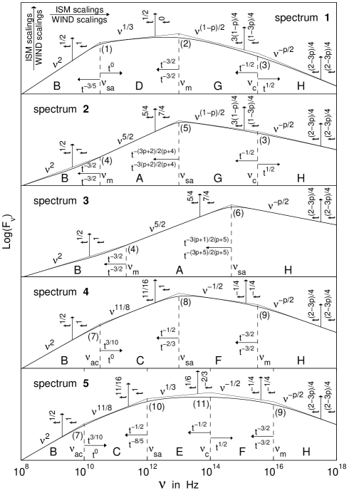
Figure 23: The different possible broad band synchrotron spectra from a relativistic blast wave, that accelerates the electrons to a power law distribution of energies. The thin solid line shows the asymptotic power law segments, and their points of intersection, where the break frequencies, $\nu_{b}$, and the corresponding flux densities, $F_{\nu_{b},{\rm ext}}$, are defined. The different PLSs are labelled A through H, while the different break frequencies are labelled 1 through 11. The temporal scalings of the power law segments and the break frequencies, for an ISM ($k=0$) or stellar wind ($k=2$) environment, are indicated by the arrows. The different spectra are labelled 1 through 5, from top to bottom. The relevant spectrum is determined by the ordering of the break frequencies. The top two panels (spectra 1 and 2) correspond to slow cooling ($\nu_{m}<\nu_{c}$). Spectrum 1 applies when $\nu_{sa}<\nu_{m}$, while spectrum 2 applies when $\nu_{m}<\nu_{sa}<\nu_{c}$. The two bottom panels (spectra 4 and 5) correspond to fast cooling ($\nu_{c}<\nu_{m}$). Spectrum 5 applies when $\nu_{sa}<\nu_{c}$, and spectrum 4 applies when $\nu_{c}<\nu_{sa}<\nu_{m}$. Spectrum 3 (middle panel) applies when $\nu_{sa}>\nu_{m},\nu_{c}$, where in this case the relative ordering of $\nu_{c}$ and $\nu_{m}$ is unimportant (i.e. spectrum 3 may apply both to slow cooling or fast cooling). From Granot and Sari (2002).

These results are valid only for $p>2$ (and for $\gamma_{max}$, the maximal electron energy, much higher than $\gamma_{min}$). If $p<2$ then $\gamma_{max}$ plays a critical role. The resulting temporal and spectral indices for slow cooling with $1<p<2$ are given by Dai and Cheng (2001) and by Bhattacharya (2001) and summarized in table 3 below. For completeness I include in this table also the cases of propagation into a wind (see §VII.5) and a jet break (see §VII.8).

	ISM	wind	Jet
$\nu<\nu_{a}$	(17p-26)/16(p-1)	(13p-18)/18(p-1)	3(p-2)/4(p-1)
$\nu_{a}<\nu<\nu_{m}$	(p+1)/8(p-1)	5(2-p)/12(p-1)	(8-5p)/6(p-1)
$\nu_{m}<\nu<\nu_{c}$	-3(p+2)/16	-(p+8)/8	-(p+6)/4
$\nu_{c}<\nu$	-(3p+10)/16	-(p+6)/8	-(p+6)/4

Table 3: $\alpha$ for slow cooling ($\nu_{a}<\nu_{m}<\nu_{c}$) into a constant density ISM, wind and jet for electron distribution with $1<p<2$.

The simple solution, that is based on a homogeneous shell approximation, can be modified by using the full BM solution and integrating over the entire volume of shocked fluid Granot et al. (1999a). Following Nakar and Piran (2003a) I discuss §VII.7.1 a simple way to perform this integration. The detailed integration yields a smoother spectrum and light curve near the break frequencies, but the asymptotic slopes, away from the break frequencies and the transition times, remain the same as in the simpler theory. Granot and Sari (2002) describe a detailed numerical analysis of the smooth afterglow spectrum including a smooth approximation for the spectrum over the transition regions (see also Gruzinov and Waxman (1999)). They also describe additional cases of ordering of the typical frequencies which were not considered earlier.

A final note on this “standard” model is that it assumes adiabaticity. However, in reality a fraction of the energy is lost and this influences over a long run the hydrodynamic behavior. This could be easily corrected by an integration of the energy losses and an addition a variable energy to Eq. 73, followed by the rest of the procedure described above Panaitescu and Kumar (2000).

VII.3 Light Curves for the early radiative phase

If the electrons’ energy is large (namely if $\epsilon_{e}$ is not far from unity), then early on during the first few hours of the afterglow there will be a radiative phase in which a significant fraction of the kinetic energy is lost via the radiative processes. One can generalize the BM solution to this radiative stage (see Cohen et al. (1998) and §VII.1). The essence of the radiative phase is that in this case the energy varies as $E\propto\Gamma$, where $\Gamma\cong(R/L)^{-3}$. Note that $L$ is calculated in terms of $M$ and the initial energy of the explosion, $E_{0}$, via $M=E_{0}/\Gamma_{0}c^{2}$, where $\Gamma_{0}$ is the initial Lorentz factor of the ejecta:

$$R(t)\cong(4ct/L)^{1/7}L,$$ (98)

$$\Gamma(t)\cong(4ct/L)^{-3/7}$$ (99)

The transition time from the radiative to the adiabatic phase takes place when the radiation losses become negligible. This happens at:

$$t_{rad}=0.17~{}{\rm hours}~{}(\epsilon_{B}/0.1)^{7/5}(\epsilon_{e}/0.1)^{7/5}E_{52}^{4/5}(\Gamma/100)^{-4/5}n_{1}^{3/5}~{}.$$ (100)

Following Sari et al. (1998b) one can use the above expressions to express the different typical frequencies and fluxes as:

$$\nu_{c} = 4.1\times 10^{14}~{}{\rm\ Hz}~{}(\epsilon_{B}/0.1)^{-3/2}E_{52}^{-4/7}(\Gamma/100)^{4/7}n_{1}^{-13/14}t_{d}^{-2/7},$$ (101)

$$\nu_{m} = 3.8\times 10^{11}~{}{\rm\ Hz}~{}(\epsilon_{B}/0.1)^{1/2}(\epsilon_{e}/0.1)^{2}E_{52}^{4/7}(\Gamma/100)^{-4/7}n_{1}^{-1/14}t_{d}^{-12/7},$$ (102)

$$F_{\nu,max} = 1.4\times 10^{3}~{}\mu{\rm J}~{}\epsilon_{B}^{1/2}E_{52}^{8/7}(\Gamma/100)^{-8/7}n_{1}^{5/14}D_{28}^{-2}t_{d}^{-3/7}\ .$$ (103)

Like in the adiabatic case this can be translated to the times of passage of the break frequencies at a given observed frequency:

$$t_{c}=0.05\times 10^{-7}~{}{\rm days}(\epsilon_{B}/0.1)^{-21/4}E_{52}^{-2}\Gamma_{2}^{2}n_{1}^{-13/4}\nu_{15}^{-7/2},$$ (104)

$$t_{m}=0.01~{}{\rm days}(\epsilon_{B}/0.1)^{7/24}(\epsilon_{e}/0.1)^{7/6}E_{52}^{1/3}\Gamma_{2}^{-1/3}\nu_{15}^{-7/12}n_{1}^{-1/24}~{}.$$ (105)

Unlike the adiabatic case, here $\nu_{c}$ must be below $\nu_{m}$. Otherwise the bulk of the electrons do not cool and the system won’t be radiative. Indeed at $t_{rad}$ (given by Eq. 100 above) $\nu_{c}=\nu_{m}$.

VII.4 Light Curve During the Newtonian transition

.

At $t\approx t_{NR}$ (see Eq. 82) the afterglow reaches the Newtonian Sedov-Taylor phase. During this phase the adiabatic hydrodynamic is described by Eq. 84. Frail et al. (2000b) calculate the synchrotron spectrum and light curve of the afterglow in this stage. The energy scaling implies that $B\propto t^{-3/5}$ and $\gamma_{e,min}\propto t^{-6/5}$. Combined together this yields $\nu_{m}\propto t^{-3}$. Using the standard assumptions of equipartition and of a power law electron’s distribution they find :

$$\nu_{c} = 10^{13}{\rm\ Hz}(\epsilon_{B}/0.3)^{-3/2}E_{51}^{-2/3}n_{1}^{-5/6}(t/t_{NR})^{-1/5},$$ (106)

$$\nu_{m} = 1{\rm GHz}(\epsilon_{B}/0.3)^{1/2}(\epsilon_{e}/0.3)^{2}n_{1}^{-1/2},$$ (107)

$$F_{\nu_{m}<\nu<\nu_{c}} = 1{\rm mJ}(\epsilon_{B}/0.3)^{3/4}(\epsilon_{e}/0.3)n_{1}^{3/4}E_{51}D_{28}^{-2}\nu^{-(p-1)/2}_{GHz}(t_{/}t_{NR})^{-3(p-1)/2+3/5}\ .$$ (108)

This late time light curve provides a simple “calorimetric” estimate of the afterglow energy at this stage (see §II.4). Additionally as the radio flux is rather large and as it varies on a scale of several month it can be used for search of orphan radio afterglows (see Levinson et al. (2002) and §VII.11.2).

VII.5 Generalizations: I. Winds

The simplest generalization of the previous models is to allow a variable circuburst density with $n(R)\propto R^{-k}$. The hydrodynamic evolution of a relativistic blast wave in such a medium was considered already in the original paper of Blandford and McKee (1976). The synchrotron light curve was considered first by Meszaros et al. (1998b) and by Dai and Lu (1999).

Chevalier and Li (1999, 2000) stressed the importance of the $n(R)\propto R^{-2}$ case which arises whenever there is a stellar wind ejected by the GRB’s progenitor prior to the burst. This arises naturally in the Collapsar model that is based on the collapse of a massive star. The calculations follow those outlines in the previous sections, with the only difference that the relations determining $R(t)$ and $\Gamma(t)$ for homogeneous circumburst medium, Eqs. 88, should be replaced by Eqs. VII.1 with $k=2$

The high initial densities in a wind density profile implies a low initial cooling frequency. Unlike the constant density case the cooling frequency here increase with time Chevalier and Li (1999). This leads to a different temporal relations between the different frequencies and cooling regimes. For example it is possible that the cooling frequency will be initially below the synchrotron self absorption frequency. Chevalier and Li (2000) consider five different evolution of the light curves for different conditions and observed frequencies. We list below the two most relevant cases, the first fits the X-ray and optical afterglows while the second is typical for the lower radio frequencies.

	$\alpha$	$\beta$
$\nu_{c}<\nu<\nu_{m}$	-1/4	-1/2
$\nu_{m},\nu_{c}<\nu$	-(3p-2)/4	$-p/2=(2\alpha-1)/3$
$\nu_{m}<\nu<\nu_{c}$	-(3p-1)/4	$-(p-1)/2=(2\alpha+1)/3$

Table 4: $\alpha$ and $\beta$ for X-ray and optical frequencies from a blast wave into a wind profile when $\nu_{a}<\nu_{c},\nu_{m},\nu$ Chevalier and Li (2000). Note that the order of the table is according to the evolution of the light curve at a fixed high observed frequency.

Note that for $\nu_{m},\nu_{c}<\nu$ both the spectral slop and the temporal evolution are similar for a wind and for a constant density profile. This poses, of course, a problem in the interpretation of afterglow light curves.

	$\alpha$	$\beta$
$\nu_{c}<\nu<\nu_{a}<\nu_{m}$	7/4	5/2
$\nu<\nu_{c}<\nu_{a}<\nu_{m}$	2	2
$\nu<\nu_{a}<\nu_{m}<\nu_{c}$	1	2
$\nu_{a}<\nu<\nu_{m}<\nu_{c}$	0	1/3
$\nu_{a}<\nu_{m}<\nu<\nu_{c}$	-(3p-1)/4	$-(p-1)/2=(2\alpha+1)/3$

Table 5: $\alpha$ and $\beta$ for radio frequencies from a blast wave into a wind profile Chevalier and Li (2000). Note that the order of the table is according to the evolution of the light curve at a fixed low observed frequency.

VII.6 Generalizations: II. Energy injection and refreshed shocks

The simple adiabatic model assumes that the energy of the GRB is constant. However, the energy could change if additional slower material is ejected behind the initial matter. This would be expected generically in the internal shock model. In this model the burst is produced by a series of collisions between shells moving at different velocities. One naturally expect here also slower moving matter that does not catch up initially with the faster moving one. However, as the initially faster moving matter is slowed down by the circum-burst matter this slower matter eventually catch up and produces refreshed shocks Rees and Mészáros (1998); Kumar and Piran (2000b); Sari and Mészáros (2000).

There are two implications for the refreshed shocks. First the additional energy injection will influence the dynamics of the blast wave Rees and Mészáros (1998); Sari and Mészáros (2000). This effect can be modelled by modifying $E$ in Eq. 73, but the effect of additional mass carrying the slower energy must be included in some cases. This would change the decay slope from the canonical one and produce a slower decay in the light curve. In the following section §VII.7 I describe a scheme for calculating the light curve resulting from a variable blast wave energy. If the additional matter is emitted sporadically then the shell collision could produce initial temporal variability in the early afterglow signal. Fox et al. (2003c), for example, suggest that refreshed shocks are the origin of the variability in the early afterglow of GRB 021004.

A second effect is the production of a reverse shock propagating into the slower material when it catches up with the faster one Kumar and Piran (2000b). This is of course in addition to the forward shock that propagates into the outer shell. This reverse shock could be episodal or long lasting depending on the profile of the additional matter. Kumar and Piran (2000b) consider two shells with energies $E_{1}$ and $E_{2}$ in the outer and the inner shells respectively. The outer shell is moving with a bulk Lorentz factor $\Gamma_{0c}\sim 5(t/day)^{3/8}$ at the (observed) time, t, of the collision. As the inner shell catches up with the outer one when both shells have comparable Lorentz factors the reverse shocks is always mildly relativistic. The calculation of the shock is slightly different than the calculation of a shell propagating into a cold material (another shell or the ISM) discussed earlier. Here the outer shell has already collided with the ISM. Hence it is hot with internal energy exceeding the rest mass energy. The reverse shock produces emission at a characteristic frequency that is typically much lower than the peak of the emission from the outer shell by a factor of $\sim 7\Gamma_{0c}^{2}(E_{2}/E_{1})^{1.1}$, and the observed flux at this frequency from the reverse shock is larger compared to the flux from the outer shell by a factor of $\sim 8(\Gamma_{0c}E_{2}/E_{1})^{5/3}$. This emission is typically in the radio or the FIR range.

Kumar and Piran (2000b) suggest that due to angular spreading the refreshed shocks produce an enhancement with a typical time scale $\delta t\sim t$. Granot et al. (2003b) stress that the fact that energy necessarily increases in refreshed shocks, the overall light curve must have a step-wise shape (above the continues power-law decline) with a break at the corresponding shocks. This behavior was seen in GRB 030329. However there the transitions are fast with $\delta t<t$. Granot et al. (2003b) point out that if the refreshed shocks take place after the jet break (as is likely the case in GRB 030329) then if the later shells remain cold and do not spread sideways we would have $\delta t\sim t_{jet}<t$. This explains nicely the fast transitions seen in this burst.

VII.7 Generalizations: III. Inhomogeneous density profiles

An interesting possibility that arose with the observation of the variable light curve of the afterglow of GRB 021004 is that the ejecta encounters surrounding matter with an irregular density profile Lazzati (2002); Nakar et al. (2003b); Heyl and Perna (2003). To explore this situation one can resort to numerical simulation of the propagation of the blast wave into a selected density profile Lazzati (2002). Instead one can attempt to model this analytically or almost analytically Nakar and Piran (2003a). The key for this analytic model is the approximation of the light curve from an inhomogeneous density profile as a series of emission from instantaneous BM solutions, each with its own external density.

VII.7.1 The light curve of a BM solution

The observed flux, at an observer time $t$, from an arbitrary spherically symmetric emitting region is given by Granot et al. (1999a):

$$F_{\nu}(t)=\frac{1}{2D^{2}}\int_{0}^{\infty}dt^{\prime}\int_{0}^{\infty}r^{2}dr\int_{-1}^{1}d(cos\theta)\frac{n^{\prime}(r)P^{\prime}_{\nu}(\nu\Lambda,r)}{\Lambda^{2}}\delta(t^{\prime}-t-\frac{r\,\,cos\theta}{c}),$$ (109)

where $n^{\prime}$ is the emitters density and $P^{\prime}_{\nu}$ is the emitted spectral power per emitter, both are measured in the fluid frame; $\theta$ is the angle relative to the line of sight, and $\Lambda^{-1}=1/\gamma(1-v\,\,cos\theta/c)$ ($v$ is the emitting matter bulk velocity) is the blue-shift factor.

Nakar and Piran (2003a) show that using the self-similar nature of the BM profile (with an external density $\propto r^{-k}$) one can reduce Eq. 109 to:

$$F_{\nu}(t)=\frac{1}{D^{2}}\int_{0}^{R_{max}(t)}A_{\nu}(R)g_{\beta}(\widetilde{t},k)dR\ .$$ (110)

The integration over $R$ is over the shock front of the BM solution. The upper limit $R_{max}$ corresponds to the shock position from where photons leaving along the line of sight reach the observer at $t$. The factor $D$ is the distance to the source (neglecting cosmological factors). $\beta$ is the local spectral index.

The factor $g_{\beta}$ is a dimensionless factor that describes the observed pulse shape of an instantaneous emission from a BM profile. The instantaneous emission from a thin shell produces a finite pulse (see §IV.2 and Fig. 14). This is generalized now to a pulse from an instantaneous emission from a BM profile. Note that even though the BM profile extends from $0$ to $R$ most of the emission arise from a narrow regions of width $\sim R/\Gamma^{2}$ behind the shock front. $g_{\beta}$ is obtained by integration Eq. 109 over $cos\theta$ and $r$, i.e. over the volume of the BM profile. It depends only on the radial and angular structure of the shell. The self-similar profile of the shell enables us to express $g_{\beta}$ as a general function that depends only on the dimensionless parameter $\widetilde{t}\equiv{(t-t_{los}(R))}/{t_{ang}(R)}$, with $t_{los}(R)$ is the time in which a photon emitted at R along the line of sight to the center reaches the observer and $t_{ang}\equiv R/2c\Gamma^{2}$. The second function, $A_{\nu}$, depends only on the conditions of the shock front along the line-of-sight. It includes only numerical parameters that remain after the integration over the volume of the shell.

When all the significant emission from the shell at radius $R$ is within the same power-law segment, $\beta$, (i.e $\nu$ is far from the break frequencies) then $A_{\nu}$ and $g_{\beta}$ are given by:

$$A_{\nu}(R)=H_{\nu}\left\{\begin{array}[]{c}R^{2}\,n^{4/3}_{ext,0}\,E_{52}^{1/3}\,M_{29}^{-1/3}\quad\nu<\nu_{m}\\ R^{2}\,n^{(5+p)/4}_{ext,0}\,E_{52}^{p}\,M_{29}^{-p}\quad\nu_{m}<\nu<\nu_{c}\\ R\,n^{(2+p)/4}_{ext,0}\,E_{52}^{p}\,M_{29}^{-p}\quad\nu>\nu_{c}\end{array}\right.\frac{erg}{sec\cdot cm\cdot Hz},$$ (111)

where $R$ is the radius of the shock front, $n_{ext}(R)$ is the external density, $E$ is the energy in the blast-wave, $M(R)$ the total collected mass up to radius $R$ and $H_{\nu}$ is a numerical factor which depends on the observed power law segment (see Nakar and Piran (2003a) for the numerical values.

$$g(\widetilde{t},\beta,k)=\left\{\begin{array}[]{c}\frac{2}{(4-k)}\int^{1+2(4-k)\widetilde{t}}_{1}\chi^{-\mu(\beta,k)}\left(1-\frac{1}{2(4-k)}+\frac{2(4-k)\widetilde{t}+1}{2(4-k)\chi}\right)^{-(2-\beta)}d\chi\quad\nu<\nu_{c}\\ (1+\widetilde{t})^{-(2-\beta)}\quad\nu>\nu_{c}\end{array}\right.,$$ (112)

where

$$\mu(\beta,k)\equiv 3\cdot(71-17k)/(72-18k)-\beta\cdot(37+k)/(24-6k).$$ (113)

This set of equations is completed with the relevant relations between the different variables of the blast wave, the observer time and the break frequencies.

These equations describe the light curve within one power law segment of the light curve. Matching between different power laws can be easily done Nakar and Piran (2003a). The overall formalism can be used to calculate the complete light curve of a BM blast wave.

VII.7.2 The light curve with a variable density or energy

The results of the previous section can be applied to study the effect of variations in the external density or in the energy of the blast-wave by approximating the solution as a series of instantaneous BM solutions whose parameters are determined by the instantaneous external density and the energy. Both can vary with time. This would be valid, of course, if the variations are not too rapid. The light curve can be expressed as an integral over the emission from a series of instantaneous BM solutions.

When a blast wave at radius $R$ propagates into the circumburst medium, the emitting matter behind the shock is replenished within $\Delta R\approx R(2^{1/(4-k)}-1)$. This is the length scale over which an external density variation relaxes to the BM solution. This approximation is valid as long as the density variations are on a larger length scales than $\Delta R$. It fails when there is a sharp density increase over a range of $\Delta R$. However, the contribution to the integral from the region on which the solution breaks is small ($\Delta R/R\ll 1$) and the overall light curve approximation is acceptable. Additionally the density variation must be mild enough so that it does not give rise to a strong reverse shock that destroys the BM profile.

A sharp density decrease is more complicated. Here the length scale in which the emitting matter behind the shock is replenished could be of the order of $R$. As an example we consider a sharp drop at some radius $R_{d}$ and a constant density for $R>R_{d}$. In this case the external density is negligible at first, and the hot shell cools by adiabatic expansion. Later the forward shock becomes dominant again. Kumar and Panaitescu (2000) show that immediately after the drop the light curve is dominated by the emission during the adiabatic cooling. Later the the observed flux is dominated by emission from $R\approx R_{d}$, and at the end the new forward shock becomes dominant. Our approximation includes the emission before the density drop and the new forward shock after the drop, but it ignores the emission during the adiabatic cooling phase.

As an example for this method Fig 24 depicts the $\nu_{m}<\nu<\nu_{c}$ light curve for a Gaussian ($\Delta R/R=0.1$) over-dense region in the ISM. Such a density profile may occur in a clumpy environment. The emission from a clump is similar to the emission from a spherically over-dense region as long as the clump’s angular size is much larger than $1/\Gamma$. Even a mild short length-scale, over-dense region (with a maximal over-density of 2) influences the light curve for a long duration (mainly due to the angular spreading). This duration depends strongly on the magnitude of the over-density.

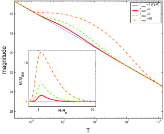
Figure 24: The light curves results from a Gaussian ($\Delta R/R=0.1$) over-dense region in the ISM. The different thick lines are for a maximal over-densities of $40$ (dashed-dot), $5$ (dashed) and $2$ (solid). The thin line is the light curve for a constant ISM density. The inset depicts the ratio of the mass, $M(R)$ over the mass of an ISM (without the over-dense region), $M_{ISM}(R)$ (from Nakar and Piran (2003a))

The calculations presented so far do not account, however, for the reverse shock resulting from density enhancement and its effect on the blast-wave. Thus the above models are limited to slowly varying and low contrast density profiles. Now, the observed flux depends on the external density, $n$, roughly as $n^{1/2}$. Thus, a large contrast is needed to produce a significant re-brightening. Such a large contrast will, however, produce a strong reverse shock which will sharply decrease the Lorentz factor of the emitting matter behind the shock, $\Gamma_{sh}$, causing a sharp drop in the emission below $\nu_{c}$ and a long delay in the arrival time of the emitted photons (the observer time is $\propto\Gamma_{sh}^{-2}$). Both factors combine to suppresses the flux and to set a strong limit on the steepness of the re-brightening events caused by density variations.

The method can be applied also to variations in the blast wave’s energy. Spherically symmetric energy variations are most likely to occur due to refreshed shocks, when new inner shells arrive from the source and refresh the blast wave Rees and Mészáros (1998); Kumar and Piran (2000b); Sari and Mészáros (2000). Once more, this approximation misses the effect of the reverse shock that arise in this case Kumar and Piran (2000b). However it enables a simple calculation of the observed light curve for a given energy profile.

VII.8 Generalizations: IV. Jets

The afterglow theory becomes much more complicated if the relativistic ejecta is not spherical. The commonly called “jets” corresponds to relativistic matter ejected into a cone of opening angle $\theta$. I stress that unlike other astrophysical jets this ejecta is non steady state and generally its width (in the direction parallel to the motion) is orders of magnitude smaller than the radius where the jet is. A “flying pancake” is a better description for these jets.

The simplest implication of a jet geometry, that exists regardless of the hydrodynamic evolution, is that once $\Gamma\sim\theta^{-1}$ relativistic beaming of light will become less effective. The radiation was initially beamed locally into a cone with an opening angle $\Gamma^{-1}$ remained inside the cone of the original jet. Now with $\Gamma^{-1}>\theta$ the emission is radiated outside of the initial jet. This has two effects: (i) An “on axis” observer, one that sees the original jet, will detect a jet break due to the faster spreading of the emitted radiation. (ii) An “off axis” observer, that could not detect the original emission will be able to see now an “orphan afterglow”, an afterglow without a preceding GRB (see §VII.11). The time of this transition is always give by Eq. 115 below with $C_{2}=1$.

Additionally the hydrodynamic evolution of the source changes when $\Gamma\sim\theta^{-1}$. Initially, as long as $\Gamma\gg\theta^{-1}$ Piran (1994) the motion would be almost conical. There isn’t enough time, in the blast wave’s rest frame, for the matter to be affected by the non spherical geometry, and the blast wave will behave as if it was a part of a sphere. When $\Gamma=C_{2}\theta^{-1}$, namely at:

$$t_{\rm jet}={1\over C_{1}}\left(l\over c\right)\left({\theta\over C_{2}}\right)^{2(4-k)\over(3-k)}$$ (114)

sideways propagation begins. The constant $C_{1}$ expresses the uncertainty at relation between the Lorentz factor and the observing time and it depends on the history of the evolution of the fireball. The constant $C_{2}$ reflects the uncertainty in the value of $\Gamma$, when the jet break begins vs. the value of opening angle of the jet $\theta$. For the important case of constant external density $k=0$ this transition takes place at:

$$t_{\rm jet}={1\,{\rm day}\over C_{1}C_{2}^{8/3}}\left({E_{\rm iso,52}\over n_{1}}\right)^{1/3}\left({\theta\over 0.1}\right)^{8/3}\ .$$ (115)

The sideways expansion continues with $\theta\sim\Gamma^{-1}$. Plugging this relations in Eq. VII.1 and letting $\Omega$ vary like $\Gamma^{-2}$ one finds that:

$$R\approx{\rm const}\ ;$$ (116)

$$\Gamma\approx(R/2t)^{1/2}\ .$$

A more detailed analysis Rhoads (1997, 1999); Piran (2000); Kumar and Panaitescu (2000) reveals that according to the simple one dimensional analytic models $\Gamma$ decreases exponentially with $R$ on a very short length scale.

Table 6 describes the parameters $\alpha$ and $\beta$ for a post jet break evolution Sari et al. (1999), The jet break usually takes place rather late, after the radiative transition. Therefore, I include in this table only the slow cooling parameters.

	$\alpha$	$\beta$
$\nu<\nu_{a}$	0	2
$\nu_{a}<\nu<\nu_{m}$	-1/3	1/3
$\nu_{m}<\nu<\nu_{c}$	-p	$-(p-1)/2=(\alpha+1)/2$
$\nu_{c}<\nu$	-p	$-p/2=\alpha/2$

Table 6: $\alpha$ and $\beta$ for slow cooling ($\nu_{a}<\nu_{m}<\nu_{c}$) after a jet break.

An important feature of the post jet-break evolution is that $\nu_{c}$, the cooling frequency becomes constant in time . This means that the high frequency (optical and X-ray ) optical spectrum does not vary after the jet-break took place. On the other hand the radio spectrum varies (see Fig. 25), giving an additional structure that confirms the interpretation of break as arising due to a sideways expansion of a jet (see e.g. Harrison et al. (1999)).

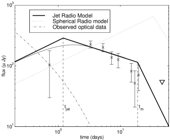
Figure 25: Observed and predicted light curve at 8.6Ghz light curves of GRB990510 (from Harrison et al. (1999)). The different behavior of the optical and radio light curves after the jet break is clearly seen.

Panaitescu and Kumar (2000) find that the jet break transition in a wind profile will be very long (up to four decades in time) and thus it will be hard to observe a jet break in such a case. On the other hand it is interesting to note that for typical values of $\alpha$ seen after a jet break ($\alpha\approx-2$) the high frequency spectral index, $\beta=\alpha/2\approx-1$, is similar to the one inferred from a spherically symmetric wind $\beta=(2\alpha+1)/3\approx-1$ Halpern et al. (1999). Note however, that the wind interpretation requires a high ($\approx 3$) p value (which may or may not be reasonable). Still from the optical observations alone it is difficult to distinguish between these two interpretations. Here the radio observations play a crucial role as the radio behavior is very different Frail et al. (2000a).

The sideways expansion causes a change in the hydrodynamic behavior and hence a break in the light curve. The beaming outside of the original jet opening angle also causes a break. If the sideways expansion is at the speed of light than both transitions would take place at the same time Sari et al. (1999). If the sideways expansion is at the sound speed then the beaming transition would take place first and only later the hydrodynamic transition would occur Panaitescu and Mészáros (1999). This would cause a slower and wider transition with two distinct breaks, first a steep break when the edge of the jet becomes visible and later a shallower break when sideways expansion becomes important.

The analytic or semi-analytic calculations of synchrotron radiation from jetted afterglows Rhoads (1999); Sari et al. (1999); Panaitescu and Mészáros (1999); Moderski et al. (2000); Kumar and Panaitescu (2000) have led to different estimates of the jet break time $t_{\rm jet}$ and of the duration of the transition. Rhoads (1999) calculated the light curves assuming emission from one representative point, and obtained a smooth ‘jet break’, extending $\sim 3-4$ decades in time, after which $F_{\nu>\nu_{m}}\propto t^{-p}$. Sari et al. (1999) assume that the sideways expansion is at the speed of light, and not at the speed of sound ($c/\sqrt{3}$) as others assume, and find a smaller value for $t_{\rm jet}$. Panaitescu and Mészáros (1999) included the effects of geometrical curvature and finite width of the emitting shell, along with electron cooling, and obtained a relatively sharp break, extending $\sim 1-2$ decades in time, in the optical light curve. Moderski et al. (2000) used a slightly different dynamical model, and a different formalism for the evolution of the electron distribution, and obtained that the change in the temporal index $\alpha$ ($F_{\nu}\propto t^{-\alpha}$) across the break is smaller than in analytic estimates ($\alpha=2$ after the break for $\nu>\nu_{m}$, $p=2.4$), while the break extends over two decades in time.

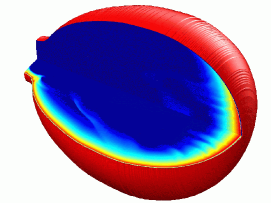
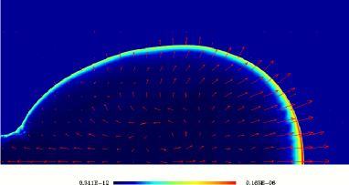
Figure 26: A relativistic jet at the last time step of the simulation Granot et al. (2001). (left) A 3D view of the jet. The outer surface represents the shock front while the two inner faces show the proper number density (lower face) and proper emissivity (upper face) in a logarithmic color scale. (right) A 2D ’slice’ along the jet axis, showing the velocity field on top of a linear color-map of the lab frame density.

The different analytic or semi-analytic models have different predictions for the sharpness of the ‘jet break’, the change in the temporal decay index $\alpha$ across the break and its asymptotic value after the break, or even the very existence a ‘jet break’ Huang et al. (2000). All these models rely on some common basic assumptions, which have a significant effect on the dynamics of the jet: (i) the shocked matter is homogeneous (ii) the shock front is spherical (within a finite opening angle) even at $t>t_{\rm jet}$ (iii) the velocity vector is almost radial even after the jet break.

However, recent 2D hydrodynamic simulations Granot et al. (2001) show that these assumptions are not a good approximation of a realistic jet. Using a very different approach Cannizzo et al. (2004) find in another set of numerical simulations a similar result - the jet does not spread sideways as much. Figure 26 shows the jet at the last time step of the simulation of Granot et al. (2001). The matter at the sides of the jet is propagating sideways (rather than in the radial direction) and is slower and much less luminous compared to the front of the jet. The shock front is egg-shaped, and quite far from being spherical. Figure 27 shows the radius $R$, Lorentz factor $\Gamma$, and opening angle $\theta$ of the jet, as a function of the lab frame time. The rate of increase of $\theta$ with $R\approx ct_{\rm lab}$, is much lower than the exponential behavior predicted by simple models Rhoads (1997, 1999); Piran (2000); Kumar and Panaitescu (2000). The value of $\theta$ averaged over the emissivity is practically constant, and most of the radiation is emitted within the initial opening angle of the jet. The radius $R$ weighed over the emissivity is very close to the maximal value of $R$ within the jet, indicating that most of the emission originates at the front of the jet, where the radius is largest, while $R$ averaged over the density is significantly lower, indicating that a large fraction of the shocked matter resides at the sides of the jet, where the radius is smaller. The Lorentz factor $\Gamma$ averaged over the emissivity is close to its maximal value, (again since most of the emission occurs near the jet axis where $\Gamma$ is the largest) while $\Gamma$ averaged over the density is significantly lower, since the matter at the sides of the jet has a much lower $\Gamma$ than at the front of the jet. The large differences between the assumptions of simple dynamical models of a jet and the results of 2D simulations, suggest that great care should be taken when using these models for predicting the light curves of jetted afterglows. Since the light curves depend strongly on the hydrodynamics of the jet, it is very important to use a realistic hydrodynamic model when calculating the light curves.

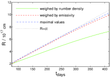
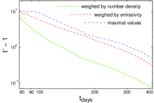
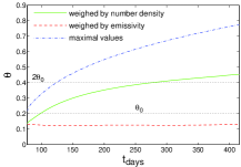
Figure 27: The radius $R$ (left frame), Lorentz factor $\Gamma-1$ (middle frame) and opening angle $\theta$ of the jet (right frame), as a function of the lab frame time in days Granot et al. (2001).

Granot et al. (2001) used 2D numerical simulations of a jet running into a constant density medium to calculate the resulting light curves, taking into account the emission from the volume of the shocked fluid with the appropriate time delay in the arrival of photons to different observers. They obtained an achromatic jet break for $\nu>\nu_{m}(t_{\rm jet})$ (which typically includes the optical and near IR), while at lower frequencies (which typically include the radio) there is a more moderate and gradual increase in the temporal index $\alpha$ at $t_{\rm jet}$, and a much more prominent steepening in the light curve at a latter time when $\nu_{m}$ sweeps past the observed frequency. The jet break appears sharper and occurs at a slightly earlier time for an observer along the jet axis, compared to an observer off the jet axis (but within the initial opening angle of the jet). The value of $\alpha$ after the jet break, for $\nu>\nu_{m}$, is found to be slightly larger than $p$ ($\alpha=2.85$ for $p=2.5$). Due to the fact that a significant fraction of the jet break occurs due to the relativistic beaming effect (that do not depend on the hydrodynamics) in spite of the different hydrodynamic behavior the numerical simulations show a jet break at roughly the same time as the analytic estimates.

VII.9 Generalizations: V. Angular Dependent Jets and the Structured Jet Model

In a realistic jet one can expect either a random or regular angular dependent structure. Here there are two dominant effects. As the ejecta slows down its Lorentz factor decreases and an observer will detect radiation from an angular region of size $\Gamma^{-1}$ (see §IV.3). At the same time the mixing within the ejecta will lead to an intrinsic averaging of the angular structure. Thus, both effects lead to an averaging over the angular structure at later times.

Several authors Lipunov et al. (2001); Rossi et al. (2002); Zhang and Mészáros (2002) suggested independently a different interpretation to the observed achromatic breaks in the afterglow light curves. This interpretation is based on a jet with a regular angular structure. According to this model all GRBs are produced by a jet with a fixed angular structure and the break corresponds to the viewing angle. Lipunov et al. (2001) considered a “universal” jet with a 3-step profile: a spherical one, a $20^{o}$ one and a $3^{o}$ one. Rossi et al. (2002) and Zhang and Mészáros (2002) considered a special profile where the energy per solid angle, $\varepsilon(\theta)$, and the Lorentz factor $\Gamma(t=0,\theta)$ are:

$$\varepsilon=\left\{\begin{array}[]{ll}\varepsilon_{c}&\;\;\;0\leq\theta\leq\theta_{c}\\ \varepsilon_{c}\big{(}\frac{\theta}{\theta_{c}})^{-a}&\;\;\;\theta_{c}\leq\theta\leq\theta_{j}\end{array}\right.$$ (117)

and

$$\Gamma=\left\{\begin{array}[]{lll}\Gamma_{c}&&\;\;\;0\leq\theta\leq\theta_{c}\\ \Gamma_{c}\big{(}\frac{\theta}{\theta_{c}})^{-b},&b>0&\;\;\;\theta_{c}\leq\theta\leq\theta{j},\end{array}\right.$$ (118)

where $\theta_{j}$ is a maximal angle and core angle, $\theta_{c}$, is introduced to avoid a divergence at $\theta=0$ and the parameters $a$ and $b$ here define the energy and Lorentz factor angular dependence. This core angle can be taken to be smaller than any other angle of interest. The power law index of $\Gamma$, $b$, is not important for the dynamics of the fireball and the computation of the light curve as long as $\Gamma(t=0,\theta)\equiv\Gamma_{0}(\theta)>\theta^{-1}$ and $\Gamma_{0}(\theta)\gg 1$.

To fit the constant energy result Frail et al. (2001); Panaitescu and Kumar (2001); Piran et al. (2001) Rossi et al. (2002) consider a specific angular structure with $a=2$. Rossi et al. (2002) approximate the evolution assuming that at every angle the matter behaves as if it is a part of a regular BM profile (with the local $\varepsilon$ and $\Gamma(t,\theta)$) until $\Gamma(t,\theta)=\theta^{-1}$. Then the matter begins to expand sideways. The resulting light curve is calculated by averaging the detected light resulting from the different angles. They find that an observer at an angle $\theta_{o}$ will detect a break in the light curve that appears around the time that $\Gamma(t,\theta_{o})=\theta_{o}^{-1}$ (see Fig. 28). A simple explanation of break is the following: As the evolution proceeds and the Lorentz factor decreases an observer will detect emission from a larger and larger angular regions. Initially the additional higher energy at small angles, $\theta<\theta_{o}$ compensates over the lower energies at larger angles $\theta>\theta_{o}$. Hence the observer detects a roughly constant energy per solid angle and the resulting light curve is comparable to the regular pre-jet break light curve. This goes on until $\Gamma^{-1}(0)=\theta_{(o)}$. After this stage an further increase in the viewing angle $\Gamma^{-1}$ will result in a decrease of the energy per unit solid angle within the viewing cone and will lead to a break in the light curve.

Figure 28: The light curves of an inhomogeneous jet observed from different angles (From Rossi et al. (2002)). From the top $\theta_{o}=0.5,\;1,\;2,\;4,\;8,\;16^{\circ}$. The break time is related only to the observer angle: $t_{b}\propto\theta_{o}^{2}$. The dashed line is the on-axis light curve of an homogeneous jet with an opening angle $2\theta_{o}$ and an energy per unit solid angle $\varepsilon(\theta_{o})$. The blow up is the time range between 4 hours and 1 month, where most of the optical observations are performed. Comparing the solid and the dashed lines for a fixed $\theta_{o}$, it is apparent that one can hardly distinguish the two models by fitting the afterglow data.

This interpretation of the breaks in the light curves in terms of the viewing angles of a standard structured jets implies a different understanding of total energy within GRB jets and of the rate of GRBs. The total energy in this model is also a constant but now it is larger as it is the integral of Eq. 117 over all viewing angles. The distribution of GRB luminosities, which is interpreted in the uniform jet interpretation as a distribution of jet opening angles is interpreted here as a distribution of viewing angles. As such this distribution is fixed by geometrical reasoning with $P(\theta_{o})d\theta_{o}\propto\sin\theta_{o}d\theta_{o}$ (up to the maximal observing angle $\theta_{j}$). This leads to an implied isotropic energy distribution of

$$P(log(E_{iso}))\propto E^{-1}_{iso}\ .$$ (119)

Guetta et al. (2003b) and Nakar et al. (2003a) find that these two distributions are somewhat inconsistent with current observations. However the present data that suffers from numerous observational biases is insufficient to reach a definite conclusions.

In order to estimate better the role of the hydrodynamics on the light curves of a structured jet Granot and Kumar (2002); Granot et al. (2003a) considered two simple models for the hydrodynamics. In the first (model 1) there is no mixing among matter moving at different angles i.e. $\varepsilon(\theta,t)=\varepsilon(\theta,t_{0})$. In the second (model 2) $\varepsilon$ is a function of time and it is averaged over the region to which a sound wave can propagate (this simulates the maximal lateral energy transfer that is consistent with causality). They consider various energy and Lorentz factors profiles and calculate the resulting light curves (see Fig. 29).

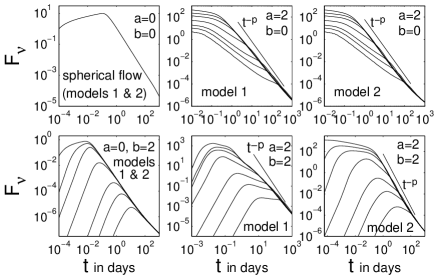
Figure 29: Light curves for structured jets (initially $\epsilon\propto\theta^{-a}$ and $\Gamma\propto\theta^{-b}$), for models 1 and 2, in the optical ($\nu=5\times 10^{14}\;$Hz), for a jet core angle $\theta_{c}=0.02$, viewing angles $\theta_{\rm obs}=0.01,0.03,0.05,0.1,0.2,0.3,0.5$, $p=2.5$, $\epsilon_{e}=\epsilon_{B}=0.1$, $n=1\;{\rm cm}^{-3}$, $\Gamma_{0}=10^{3}$, and $\epsilon_{0}$ was chosen so that the total energy of the jet would be $10^{52}\;$erg (GK). A power law of $t^{-p}$ is added in some of the panels, for comparison. From Granot et al. (2003a)

Granot and Kumar (2002) find that the light curves of models 1 and 2 are rather similar in spite of the different physical assumptions. This suggests that the widening of the viewing angle has a more dominant effect than the physical averaging. For models with a constant energy and a variable Lorentz factor ($(a,b)=(0,2)$) the light curve initially rises and there is no jet break, which is quite different from observations for most afterglows. For $(a,b)=(2,2),\,(2,0)$ they find a jet break at $t_{j}$ when $\Gamma(\theta_{o})\sim\theta_{o}^{-1}$. For $(a,b)=(2,2)$ the value, $\alpha_{1}$, of the temporal decay slope at $t<t_{j}$ increases with $\theta_{o}$, while $\alpha_{2}=\alpha(t>t_{j})$ decreases with $\theta_{o}$. This effect is more prominent in model 1, and appears to a lesser extent in model 2. This suggests that $\delta\alpha=\alpha_{1}-\alpha_{2}$ should increase with $t_{j}$, which is not supported by observations. For $(a,b)=(2,0)$, there is a flattening of the light curve just before the jet break (also noticed by Rossi et al. (2002)), for $\theta_{o}>3\theta_{c}$. Again, this effect is larger in model 1, compared to model 2 and again this flattening is not seen in the observed data.

Clearly a full solution of an angular dependent jet requires full numerical simulations. Kumar and Granot (2003) present a simple 1-D model for the hydrodynamics that is obtained by assuming axial symmetry and integrating over the radial profile of the flow, thus considerably reducing the computation time. The light curves that they find resemble those of models 1 and 2 above indicating that these crude approximations are useful. Furthermore they find relatively little change in $\epsilon(\theta)$ within the first few days, suggesting that model 1 is an especially useful approximation for the jet dynamics at early times, while model 2 provides a better approximation at late times.

VII.10 Afterglow Polarization - a tool that distinguished between the different jet models

Synchrotron emission from a jet (in which the spherical symmetry is broken) would naturally produce polarized emission Gruzinov (1999); Ghisellini and Lazzati (1999); Sari (1999b). Moreover, the level and the direction of the polarization are expected to vary with time and to give observational clues on the geometrical structure of the emitting jet and our observing angle with respect to it.

The key feature in the determination of the polarization during the afterglow is the varying Lorentz factor and (after jet break) varying jet width. This changes changes the overall geometry (see Fig. 16) and hence the observer sees different geometries Sari (1999b); Hurley et al. (2002e). Initially, the relativistic beaming angle $1/\Gamma$ is narrower than the physical size of the jet $\theta_{0}$, and the observer see a full ring and therefore the radial polarization averages out (the first frame, with $\Gamma\theta_{0}=4$ of the left plot in Fig. 30). As the flow decelerates, the relativistic beaming angle $1/\Gamma$ becomes comparable to $\theta_{0}$ and only a fraction of the ring is visible; net polarization is then observed. Assuming, for simplicity, that the magnetic field is along the shock then the synchrotron polarization will be radially outwards. Due to the radial direction of the polarization from each fluid element, the total polarization is maximal when a quarter ($\Gamma\theta_{0}=2$ in Figure 30) or when three quarters ($\Gamma\theta_{0}=1$ in Figure 30) of the ring are missing (or radiate less efficiently) and vanishes for a full and a half ring. The polarization, when more than half of the ring is missing, is perpendicular to the polarization direction when less than half of it is missing.

Figure 30: Left: Shape of the emitting region. The dashed line marks the physical extent of the jet, and solid lines give the viewable region $1/\gamma$. The observed radiation arises from the gray shaded region. In each frame, the percentage of polarization is given at the top right and the initial size of the jet relative to $1/\Gamma$ is given on the left. The frames are scaled so that the size of the jet is unity. Right: Observed and theoretical polarization light curves for three possible offsets of the observer relative to the jet axis Observational data for GRB 990510 is marked by crosses (x), assuming $t_{jet}=1.2$ days. The upper limit for GRB 990123 is given by a triangle, assuming $t_{jet}=2.1$ days (from Sari (1999b)).

At late stages the jet expands sideways and since the offset of the observer from the physical center of the jet is constant, spherical symmetry is regained. The vanishing and re-occurrence of significant parts of the ring results in a unique prediction: there should be three peaks of polarization, with the polarization position angle during the central peak rotated by $90^{\circ}$ with respect to the other two peaks. In case the observer is very close to the center, more than half of the ring is always observed, and therefore only a single direction of polarization is expected. A few possible polarization light curves are presented in Fig. 30.

The predicted polarization from a structured jet is drastically different from the one from a uniform jet, providing an excellent test between the two models Rossi et al. (2004). Within the structured jet model the polarization arises due to the gradient in the emissivity. This gradient has a clear orientation. The emissivity is maximal at the center of center of the jet and is decreases monotonously outwards. The polarization will be maximal when the variation in the emissivity within the emitting beam are maximal. This happens around the jet break when $\theta_{obs}\sim\Gamma^{-1}$ and the observed beam just reaches the center. The polarization expected in this case is around 20% Rossi et al. (2004) and it is slightly larger than the maximal polarization from a uniform jet. As the direction of the gradient is always the same (relative to a given observer) there should be no jumps in the direction of the polarization.

According to the patchy shell model Kumar and Piran (2000a) the jet can includes variable emitting hot spots. This could lead to a fluctuation in the light curve (as hot spots enter the observed beam) and also to corresponding fluctuations in the polarization Granot (2003); Nakar and Oren (2003). There is a clear prediction Nakar et al. (2003b); Nakar and Oren (2003) that if the fluctuations are angular fluctuations have a typical angular scale $\theta_{f}$ then the first bump in the light curve should take place on the time when $\Gamma^{-1}\sim\theta_{f}$ (the whole hot spot will be within the observed beam). The following bumps in the light curve should decrease in amplitude (due to statistical fluctuations). Nakar and Oren (2003) show analytically and numerically that the jumps in the polarization direction should be random, sharp and accompanied by jumps in the amount of polarization.

VII.11 Orphan Afterglows

Orphan afterglows arise as a natural prediction of GRB jets. The realization that GRBs are collimated with rather narrow opening angles, while the following afterglow could be observed over a wider angular range, led immediately to the search for orphan afterglows: afterglows which are not associated with observed prompt GRB emission. While the GRB and the early afterglow are collimated to within the original opening angle, $\theta_{j}$, the afterglow can be observed, after the jet break, from a viewing angle of $\Gamma^{-1}$. The Lorentz factor, $\Gamma$, is a rapidly decreasing function of time. This means that an observer at $\theta_{obs}>\theta_{j}$ couldn’t see the burst but could detect an afterglow once $\Gamma^{-1}=\theta_{obs}$. As the typical emission frequency and the flux decrease with time, while the jet opening angle $\theta$ increases, this implies that observers at larger viewing angles will detect weaker and softer afterglows. X-ray orphan afterglows can be observed several hours or at most a few days after the burst (depending of course on the sensitivity of the detector). Optical afterglows (brighter than 25th mag ) can be detected in R band for a week from small ($\sim 10^{\circ}$) angles away from the GRB jet axis. On the other hand, at very late times, after the Newtonian break, radio afterglows could be detected by observers at all viewing angles.

The search for orphan afterglows is an observational challenge. One has to search for a $~{}10^{-12}$ergs/sec/cm² signal in the X-ray , a 23th or higher magnitude in the optical or a mJy in radio (at GHz) transients. Unlike afterglow searches that are triggered by a well located GRB for the orphan afterglow itself there is no information where to search and confusion with other transients is rather easy. So far there was no detection of any orphan afterglow in any wavelength.

Rhoads (1997) was the first to suggest that observations of orphan afterglows would enable us to estimate the opening angles and the true rate of GRBs. Dalal et al. (2002) have pointed out that as the post jet-break afterglow light curves decay quickly, most orphan afterglows will be dim and hence undetectable. They point out that if the maximal observing angle, $\theta_{max}$, of an orphan afterglow will be a constant factor times $\theta_{j}$ the ratio of observed orphan afterglows, $R_{orph}^{obs}$, to that of GRBs, $R_{GRB}^{obs}$, will not tell us much about the opening angles of GRBs and the true rate of GRBs, $R_{GRB}^{true}\equiv f_{b}R_{GRB}^{obs}$. However as we see below this assumption is inconsistent with the constant energy of GRBs that suggests that all GRBs will be detected to up to a fixed angle which is independent of their jet opening angle.

VII.11.1 Optical Orphan Afterglow

Optical orphan afterglow is emitted at a stage when the outflow is still relativistic. The observation that GRBs have a roughly constant total energy Frail et al. (2001); Panaitescu and Kumar (2001); Piran et al. (2001) and that the observed variability in the apparent luminosity arises mostly from variation in the jet opening angles leads to a remarkable result: The post jet-break afterglow light curve is universal Granot et al. (2002). Fig. 31 depicts this universal light curve. This implies that for a given redshift, $z$, and a given limiting magnitude, $m$, there will be a fixed $\theta_{max}(z,m)$ (independent of $\theta_{j}$, for $\theta_{j}<\theta_{max}$) from within which orphan afterglow can be detected.

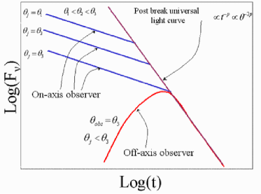
Figure 31: A schematic afterglow light curve. While the burst differ before the jet break (due to different opening angles, the light curve coincide after the break when the energy per unit solid angle is a constant.

This universal post jet-break light curve can be estimated from the observations Totani and Panaitescu (2002) or alternatively from first principles Nakar et al. (2002) . An observer at $\theta_{obs}>\theta_{j}$ will (practically) observe the afterglow emission only at $t_{\theta}$ when $\Gamma=\theta_{obs}^{-1}$. Using Eq. 115 and the fact that $\Gamma\propto t^{-1/2}$ after the jet break (Eq. VII.8) one can estimate the time, $t_{\theta}$ when a emission from a jet would be detected at $\theta_{obs}$:

$$t_{\theta}=A(\theta_{obs}/\theta_{j})^{2}t_{jet}\ ,$$ (120)

where $A$ is a factor of order unity, and $t_{jet}$ is the time of the jet break (given by Eq. 115). The flux at this time is estimated by substitution of this value into the post-jet-break light curve (see Nakar et al. (2002) for details):

$$F(\theta_{obs})=F_{0}f(z)\theta_{obs}^{-2p}\ ,$$ (121)

where $F_{0}$ is a constant and $f(z)=(1+z)^{1+\beta}D_{L28}^{-2}$ includes all the cosmological effects and $D_{L28}$ is the luminosity distance in units of $10^{28}$cm. One notices here a very strong dependence on $\theta_{obs}$. The peak flux drops quickly when the observer moves away from the axis. Note also that this maximal flux is independent of the opening angle of the jet, $\theta_{j}$. The observations of the afterglows with a clear jet break (GRB990510 Harrison et al. (1999); Stanek et al. (1999), and GRB000926 Harrison et al. (2001)) can be used to calibrate $F_{0}$.

Now, using Eq. 121, one can estimate $\theta_{max}(z,m)$ and more generally the time, $(t_{obs}(z,\theta,m)$ that a burst at a redshift, $z$, can be seen from an angle $\theta$ above a limiting magnitude, $m$:

$$t_{obs}(z,\theta,m)\approx{At_{jet}\over\theta_{j}^{2}}(\theta_{max}^{2}-\theta_{obs}^{2})\ .$$ (122)

One can then proceed and integrate over the cosmological distribution of bursts (assuming that this follows the star formation rate) and obtain an estimate of the number of orphan afterglows that would appear in a single snapshot of a given survey with a limiting sensitivity $F_{lim}$:

$$N_{orph}=\int_{0}^{\infty}{n(z)\over(1+z)}{dV(z)\over dz}dz\times\int_{\theta_{j}}^{\theta_{max}(z,m)}t_{obs}(z,\theta,m)\theta d\theta\propto(F_{0}/F_{lim})^{2/p}\ .$$ (123)

where n(z) is the rate of GRBs per unit volume and unit proper time and dV(z) is the differential volume element at redshift $z$. Note that modifications of this simple model may arise with more refined models of the jet propagation Granot et al. (2002); Nakar et al. (2002).

The results of the intergration of Eq. 123 are depicted in Fig. 32.

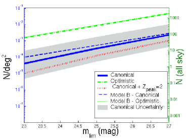
Figure 32: The number of observed orphan afterglows per square degree (left vertical scale) and in the entire sky (right vertical scale), in a single exposure, as a function of the limiting magnitude for detection. The thick lines are for model A with three different sets of parameters: i) Our “canonical” normalization $F_{0}=0.003\,\mu{\rm Jy}$, $z_{peak}=1$, $\theta_{j}=0.1$ (solid line). The gray area around this line corresponds an uncertainty by a factor of 5 in this normalization. ii) Our most optimistic model with a relatively small $\theta_{j}=0.05$ and a large $F_{0}=0.015\,\mu{\rm Jy}$ (dashed-dotted line). iii) The same as our “canonical” model, except for $z_{peak}=2$ (dotted line). The thin lines are for model B, where the solid line is for our “optimistic” parameters, while the dashed line is for our “canonical” parameters. Both models are similar for the “optimistic” parameters while model B predicts slightly more orphan afterglows then model A for the “canonical” parameters. From Nakar et al. (2002)

Clearly the rate of a single detection with a given limiting magnitude increases with a larger magnitude. However, one should ask what will be the optimal strategy for a given observational facility: short and shallow exposures that cover a larger solid angle or long and deep ones over a smaller area. The exposure time that is required in order to reach a given limiting flux, $F_{lim}$, is proportional to $F_{lim}^{-2}$. Dividing the number density of observed orphan afterglows (shown in Fig. 32) by this time factor results in the rate per square degree per hour of observational facility. This rate increases for a shallow surveys that cover a large area. This result can be understood as follows. Multiplying Eq. 123 by $F_{lim}^{2}$ shows that the rate per square degree per hour of observational facility $\propto F_{lim}^{2-2/p}$. For $p>1$ the exponent is positive and a shallow survey is preferred. The limiting magnitude should not be, however, lower than $\sim$ 23rd as in this case more transients from on-axis GRBs will be discovered than orphan afterglows.

Using these estimates Nakar et al. (2002) find that with their most optimistic parameters 15 orphan afterglows will be recorded in the Sloan Digital Sky Survey (SDSS) (that covers 10⁴ square degrees at 23rd mag) and 35 transients will be recorded in a dedicated 2m class telescope operating full time for a year in an orphan afterglow search. Totani and Panaitescu (2002) find a somewhat higher rate (a factor $\sim 10$ above the optimistic rate). About 15% of the transients could be discovered with a second exposure of the same area provided that it follows after 3, 4 and 8 days for $m_{lim}=23$, 25 and 27. This estimate does not tackle the challenging problem of identifying the afterglows within the collected data. Rhoads (2001) suggested to identify afterglow candidates by comparing the multi-color SDSS data to an afterglow template. One orphan afterglow candidate was indeed identified using this technique Vanden Berk et al. (2002). However, it turned out that it has been a variable AGN Gal-Yam et al. (2002). This event demonstrates the remarkable observational challenge involved in this project.

VII.11.2 Radio Orphan Afterglow

After the Newtonian transition the afterglow is expanding spherical. The velocities are at most mildly relativistic so there are no relativistic beaming effects and the afterglow will be observed from all viewing angles. This implies that observations of the rate of orphan GRB afterglows at this stage will give a direct measure of the beaming factor of GRBs. Upper limits on the rate of orphan afterglows will provide a limit on the beaming of GRBs Perna and Loeb (1998). However, as I discuss shortly, somewhat surprisingly, upper limits on the rate of orphan radio afterglow (no detection of orphan radio afterglow) provide a lower (and not upper) limit on GRB beaming Levinson et al. (2002).

Frail et al. (2000b) estimate the radio emission at this stage using the Sedov-Taylor solution for the hydrodynamics (see §VII.4). They find that the radio emission at GHz will be around 1 mJy at the time of the Newtonian transition (typically three month after the burst) and it will decrease like $t^{-3(p-1)/2+3/5}$ (see Eq. 106). Using this limit one can estimate the rate of observed orphan radio afterglow within a given limiting flux. The beaming factor $f^{-1}_{b}$ arises in two places in this calculations. First, the overall rate of GRBs: $R_{GRB}^{true}\equiv f_{b}R_{GRB}^{obs}$, increases with $f_{b}$. Second the total energy is proportional to $f_{b}^{-1}$ hence the flux will decrease when $f_{B}$ increases. The first factor implies that the rate of orphan radio afterglows will increase like $f_{b}$. To estimate the effect of the second factor Levinson et al. (2002) use the fact that (for a fixed observed energy) the time that a radio afterglow is above a given flux is proportional to $E^{10/9}$ in units of the NR transition time which itself is proportional to $E^{1/3}$. Overall this is proportional to $E^{13/9}$ and hence to $f_{b}^{-13/9}$. To obtain the overall effect of $f_{b}$ Levinson et al. (2002) integrate over the redshift distribution and obtain the total number of orphan radio afterglow as a function of $f_{b}$. For a simple limit of a shallow survey (which is applicable to current surveys) typical distances are rather “small”, i.e. less than 1Gpc and cosmological corrections can be neglected. In this case it is straight forwards to carry the integration analytically and obtain the number of radio orphan afterglows in the sky at any given moment Levinson et al. (2002):

$$N_{R}\simeq 10^{4}f_{b}^{5/6}(R/0.5)\left(\frac{f_{\nu min}}{5mJy}\right)^{-3/2}\left(\frac{\epsilon_{e}}{0.3}\right)^{3/2}\left(\frac{\epsilon_{B}}{0.03}\right)^{9/8}n_{-1}^{19/24}E_{\rm iso,54}^{11/6}\nu_{9}^{-3/4}(t_{i}/3t_{NR})^{-7/20}.$$ (124)

where $R$ is the observed rate of GRBs per Gpc³ per year, and $t_{i}$ is the time in which the radio afterglow becomes isotropic.

Levinson et al. (2002) search the FIRST and NVSS surveys for point-like radio transients with flux densities greater than 6 mJy. They find 9 orphan candidates. However, they argue that the possibility that most of these candidates are radio loud AGNs cannot be ruled out without further observations. This analysis sets an upper limit for the all sky number of radio orphans, which corresponds to a lower limit $f_{b}^{-1}>10$ on the beaming factor. Rejection of all candidates found in this search would imply $f_{b}^{-1}>40$ Guetta et al. (2003b).

VII.12 Generalizations: VI. Additional Physical Processes

With the development of the theory of GRB afterglow it was realized that several additional physical ingredients may influence the observed afterglow light emission. In this section I will review two such processes: (i) Pre acceleration of teh surrounding matter by the prompt $\gamma$-rays emission and (ii) Decay of neutrons within the outflow.

VII.12.1 Pre-acceleration

The surrounding regular ISM or even stellar wind is optically thin to the initial $\gamma$-rays pulse. Still the interaction of the pulse and the surrounding matter may not be trivial. Thompson and Madau (2000) pointed out that a small fraction of the $\gamma$-rays radiation will be Compton scattered on the surrounding electrons. The backscattered photons could now interact with the outwards going $\gamma$-rays flux and produce pairs. The pairs will increase the rate of backscattering and this could lead to an instability. When sufficient number of pairs will be produced the surrounding matter will feel a significant drag by the $\gamma$-rays flux and it will be accelerated outwards Madau and Thompson (2000). These pre-acceleration of the ambient medium could have several implications to the early afterglow Mészáros et al. (2001); Beloborodov (2002b).

The key issue is that while the optical depth of the surrounding medium (as “seen” the $\gamma$-rays photons) is very small, the mean free path of an ambient electron within the $\gamma$-rays photons is large (at small enough radius) and each electron scatters many photons. While the medium absorbs only a small fraction of the prompt $\gamma$-rays energy, the effect of this energy can be significant. Beloborodov (2002a) characterizes the interaction of the $\gamma$-rays radiation front with the surrounding medium by a dimensionless parameter:

$$\eta=\frac{\sigma_{T}E_{iso}}{4\pi R^{2}m_{e}c^{2}}=6.5E_{52}R_{16}^{-2}\ ,$$ (125)

the energy that a single electron scatters relative to its rest mass. Beloborodov (2002b) calculates the Lorentz factor of the ambient medium and the number of pairs per initial electron as functions of $\eta$. where $\eta_{load}=20-30$, depending on the spectrum of the gamma-rays, $\eta_{acc}=5\eta_{load}=100-150$, and $f_{acc}=[\exp(\eta_{acc}/\eta_{load})+\exp(-\eta_{acc}/\eta_{load})]/2=74$.

If $\eta<\eta_{load}\approx 20-30$, depending on the spectrum of the gamma-rays, the medium remains static and $e^{\pm}$-free. When the front has $\eta>\eta_{load}$, a runaway $e^{\pm}$ loading occurs. The number of loaded pairs depends exponentially on $\eta$ as long as $\eta<\eta_{acc}=5\eta_{load}=100-150$. The medium is accelerated if $\eta>\eta_{acc}$. $\eta_{acc}$ is around 100 because the electrons are coupled to the ambient ions, and and the other hand the loaded $e^{\pm}$ increase the number of scatters per ion. At $\eta=\eta_{gap}\approx 3\times 10^{3}$, the matter is accelerated to a Lorentz factor $\Gamma_{ambient}$ that exceeds the Lorentz factor of the ejecta. It implies that the radiation front pushes the medium away from the ejecta and opens a gap.

As the GRB radiation front expands, the energy flux and hence $\eta$ decreases $\propto R^{-2}$. $\eta$ passes through $\eta_{gap}$, $\eta_{acc}$, and $\eta_{load}$ at $R_{gap}$, $R_{acc}$, and $R_{load}$, respectively. These three characteristic radii define four stages:

i. $R<R_{gap}\approx R_{acc}/3$: The ejecta moves in a cavity produced by the radiation front with $\Gamma_{ambient}>\Gamma_{ejecta}$.

II. $R_{gap}<R<R_{acc}\approx 3\times 10^{15}{\rm~{}cm}E_{52}^{1/2}{\rm~{}cm}$: The ejecta sweeps the $e^{\pm}$-rich medium that has been preaccelerated to $1\ll\Gamma_{ambient}<\Gamma_{ejecta}$.

III. $R_{acc}<R<R_{load}\approx 2.3R_{acc}$. The ejecta sweeps the “static” medium ($\Gamma_{ambient}\approx 1$) which is still dominated by loaded $e^{\pm}$.

IV. $R>R_{load}$. The ejecta sweeps the static pair-free medium.

This influence of the $\gamma$-rays on the surrounding matter may modify the standard picture of interaction of external shocks with the surrounding medium (see §VI.3.1. This depends mostly on the relation between $R_{ext}$ and $R_{gap}\approx 10^{15}E_{52}^{1/2}$ cm. If $R_{ext}>R_{gap}$ this effect won’t be important. However, if $R_{ext}<R_{gap}$ then effective decceleration will begin only at $R_{gap}$. At $R<R_{gap}$ the ejecta freely moves in a cavity cleared by the radiation front and only at $R=R_{gap}$ the blast wave gently begins to sweep the preaccelerated medium with a small relative Lorentz factor. With increasing $R>R_{gap}$, $\Gamma_{ambient}$ falls off quickly, and it approaches $\Gamma_{ambient}=1$ at $R=R_{acc}\approx 3R_{gap}$ as $\Gamma_{ambient}=(R/R_{acc})^{-6}$. Thus, after a delay, the ejecta suddenly “learns” that there is a substantial amount of ambient material on its way. This resembles a collision with a wall and results in a sharp pulse (see Fig. 33).

Figure 33: Afterglow from a GRB ejecta decelerating in a wind of a Wolf-Rayet progenitor with $\dot{M}=2\times 10^{-5}M_{\odot}$ yr^-1 and $w=10^{3}$ km s^-1. The burst has an isotropic energy $E=10^{53}$ erg) and a thin ejecta shell with kinetic energy $E=10^{53}$ erg and a Lorentz factor $\Gamma=200$. Dashed curves show the prediction of the standard model that neglects the impact of the radiation front, and solid curves show the actual behavior. Two extreme cases are displayed in the figure: $\eta=0$ (adiabatic blast wave) and $\eta=1$ (radiative blast wave). Four zones are marked: I - $R<R_{gap}$ (the gap is opened), II - $R_{gap}<R<R_{acc}$ (the gap is closed and the ejecta sweeps the relativistically preaccelerated $e^{\pm}$-loaded ambient medium), III - $R_{acc}<R<R_{load}$ ($e^{\pm}$-loaded ambient medium with $\Gamma_{ambient}\approx 1$), and IV - $R>R_{load}$ (pair-free ambient medium with $\Gamma_{ambient}\approx 1$). The radie are measured in units of $R_{acc}\approx 10^{16}$ cm. Top panel: dissipation rate. Bottom panel: synchrotron peak frequency (assuming $\epsilon_{B}=0.1$) in units of $m_{e}c^{2}/h$. From Beloborodov (2002a)

While $R_{gap}$ does not depend on the external density $R_{ext}$ does (see Eq. 64). The condition $R_{ext}<R_{gap}$ implies:

$$E_{52}^{1/6}n_{1}^{1/3}\Gamma^{2/3}_{100}>0.02$$ (126)

Thus it requires a dense external medium and large initial Lorentz factor. Otherwise $R_{gap}$ is too large and the deceleration takes place after the gap is closed. Hence the conditions for pre-acceleration will generally occur if the burst takes place in a dense circumburst regions, like in a Wolf-Rayet progenitor Beloborodov (2002b). Kumar and Panaitescu (2003) elaborate on this model and find that the observational limits by LOTIS and ROTSE on prompt emission from various burst limit the ambient ISM density (within $10^{16}$cm to less than $10^{3}{rmcm}^{-3}$. Similarly the find that in case of a wind the progenitors mass loss to wind’s velocity ratio is below $10^{-6}M_{\odot}$/yr/(10³km/sec).

VII.12.2 Neutron decoupling and decay

Derishev et al. (2001, 1999) pointed out that neutrons that are included initially in the fireball will change its dynamics and modify the standard afterglow evolution. While the protons slow down due to the interaction with the surrounding matter the neutrons will coast freely after they decouple with $\Gamma_{n}$, which equals to the Lorentz factor while decoupling took place.

At

$$R_{decay}\approx 0.3\times 10^{16}{\rm cm}(\Gamma_{n}/100)$$ (127)

the neutrons decay. A new baryonic shell forms ahead of the original fireball shell, with energy comparable to the initial energy of the protons’ shell (this depends, of course, on the initial ratio of neutrons to protons). At this stage the neutrons front that is not slowed down like the rest of the fireball is at a distance:

$$\Delta R=R(1/2\Gamma^{2}-1/2Gamma^{2}_{n})\ ,$$ (128)

from the fireball front, where $\Gamma$ is the current Lorentz factor of the fireball.

Once more the situation depends on whether $R_{decay}$ is smaller or larger than $R_{ext}$, the original deceleration radius. If $R_{decay}<R_{ext}$:

$$E_{5}2^{1/3}n_{1}^{-1/3}\Gamma^{-2/3}_{100}(\Gamma_{n}/300)^{-1}<0.06\ ,$$ (129)

the decaying neutron products will mix with the original protons and won’t influence the evolution significantly (apart from adding their energy to the adiabatic fireball energy). Otherwise, they situation depends on $\Gamma_{n}$ the Lorentz factor at decoupling.

Pruet and Dalal (2002) consider a situation in which the neutron decouple with a low $\Gamma_{n}$. In this case one will get a delayed shock scenario when the neutronic decay produce will eventually catch up with the slowing down protons (when their Lorentz factor is of order $\Gamma_{n}$. Along the same line of thought Dalal et al. (2002) suggest that a large neutronic component that may exist within the initial fireball material may help to eliminate the baryon load problem Shemi and Piran (1990).

Beloborodov (2003) considers a situation when $\Gamma_{n}\approx\Gamma_{0}$, the initial Lorentz factor of the protons. In this case the decaying neutrons’ products will be ahead of the shell of the protons. The decaying products will interact with the surrounding matter and will begin to slow down. There will be a triple interaction between the two shells and the surrounding ambient medium (resembling to some extend the pre-acceleration scenario described earlier) . This will take place at radii of a few times $R_{decay}$ and at an observed time of a few $\times R_{decay}/2c\Gamma^{2}\approx{\rm afewseconds}/(\Gamma_{n}/300)$, i.e. extremely early. This will produce brightening when the fronts pass $R_{decay}$.

The neutrons could also influence the behavior of the relativistic flow during the prompt (internal shocks) phase. Specifically inelastic collisions between differentially streaming protons and neutrons can produce pions and eventually $\nu_{\mu}$ of  10 GeV as well as $\nu_{e}$ of  5 GeV Bahcall and Mészáros (2000); Mészáros and Rees (2000). These neutrino fluxes could produce $\sim 7$ events/year in km3 neutrino detectors. GeV photons will also be produced but it is unlikely that they could be detected.

VIII Additional Emission from GRBs

VIII.1 TeV $\gamma$-rays 

Hurley (1994) reported on detection of 18 GeV photons from GRB 940217. Milagrito - A TeV detector - discovered a possible TeV signal coincident with GRB 970417 Atkins et al. (2000). González et al. (2003) discovered a high energy tail that extended up to 200 MeV from GRB 941017.

A natural source for high energy $\gamma$-rays is the SSC (Synchrotron self Compton) component produced by IC from the burst itself or from the afterglow Mészáros and Rees (1994); Meszaros et al. (1994). The SSC photons energy should be $\gamma_{e}^{2}$ higher than the synchrotron photons. Typical random Lorentz factors of electrons, $\gamma_{e}$, within internal shocks are of order a thousand (in the fluid’s rest frame). This implies that if the observed $\gamma$-rays emission is produced by synchrotron in internal shocks then the IC emission would produce a second peak around a few hundred GeV. This would be the analogue of the high energy component observed in Blazars. Note that emission above $\sim 10-100$GeV might be self absorbed by pair production with the source Papathanassiou and Meszaros (1996); Pilla and Loeb (1998); Guetta and Granot (2003).

The SSC component would be even higher from the early afterglow. The synchrotron emission from the forward shock is expected to be around 10 keV (if the observed early afterglow is indeed produced by the external shocks). With a Lorentz factor of a typical electron around $10^{5}$ the expected SSC component should be around $100$TeV. Finally the reverse shock emission is expected to produce 100 eV photons Sari and Piran (1999c). With typical electrons Lorentz factor of a few thousand this should correspond to SSC photons with typical energy of 100 MeV. Depending on the relevant Y parameter the fluxes of these high energy components should be comparable or even larger than the prompt GRB $\gamma$-rays fluxes. This emission should be simultaneous with the GRB emission. It is also possible that the forward shock electrons will IC reverse shocks photons. It is likely that this is the cause of the high energy emission seen in GRB 941017 Pe’er and Waxman (2004); Piran et al. (2003).

Other mechanisms can produce high energy emission as well. Vietri (1997) suggested that as GRB can accelerate protons up to $10^{20}$eV (see §VIII.3 below). These protons can emit 0.01 of the GRB energy as high energy $\gamma$-rays with energies up to 300 GeV. Bottcher and Dermer (1998) considered the synchrotron spectrum resulting from high energy protons and leptons produced in cascade initiated by photo-pion production. They predict a significant flux of 10Mev-100GeV photons.

While the high energy photons flux could be significant these photons might not be detectable on earth. The high energy photon flux above 1 TeV would be attenuated significantly due to pair production of such high energy photons with the intergalactic NIR flux Gould and Schréder (1967). Dai and Lu (2002) suggest that secondary emission produced via these interaction (upscattering of the CMB by the produced pairs) would still point towards the initial direction and hence might be detectable as a delayed GeV emission. However, even a tiny intergalactic magnetic field ($>10^{-22}$G would be sufficient to deflect the electrons and dilute these signal Guetta and Granot (2003).

VIII.2 Neutrinos

Neutrinos can be produced in several regions within GRB sources. First some models, like the Collapsar model or the neutron star merger model predict ample ($\sim 10^{53}$ ergs) production of low (MeV) neutrinos. However, no existing or planned detector could see those from cosmological distances. Furthermore, this signal will be swamped in rate by the much more frequent SN neutrino signals which would typically appear closer.

However, GRBs could be detectable sources of high energy neutrinos, with energies ranging from $10^{14}$eV to $10^{17}$eV. These neutrinos are produced by internal or external shocks of the GRB process itself and hence are independent of the nature of the progenitor.

To understand the process of neutrino emission recall that neutrinos are “best” produced in nature following pions production in proton-photon or proton-proton collisions. The proton-photon process requires that the photon’s energy is around the $\Delta$ resonance in the proton’s energy frame: namely at $\sim 200$MeV. The resulting pion decays emitting neutrinos with a typical energy of $\sim 50$ MeV in the proton’s rest frame. If the proton is moving relativistically, with a Lorentz factor $\gamma_{p}$ within the laboratory frame the required photon energy in the lab frame is smaller by a factor of $\gamma_{p}$ and the resulting neutrino energy is larger by a factor of $\gamma_{p}$. Depending on the surrounding environment very energetic pions may lose some of their energy before decaying producing a “cooling break” in the neutrino spectrum. In this case the resulting neutrinos’ energy will be lower than this naive upper limit.

Within GRBs protons are accelerated up to $10^{20}$eV Waxman (1995); Vietri (1995). The relevant Lorentz factors of these protons range from $\Gamma$ up to $10^{11}$ (at the very high energy tail of the protons distribution). Thus we expect neutrinos up to $10^{19}$eV provided that there is a sufficient flux of photons at the relevant energies so that the pions can be produced and there are no energy loses to the pions.

Paczynski and Xu (1994) and Waxman and Bahcall (1997) calculated the flux of VHE neutrinos from internal shocks. They found that a significant flux of $\sim 10^{14}$eV neutrinos can be produced by interaction of the accelerated internal shocks protons with the GRB photons. Guetta et al. (2001b) estimate that on average each GRB produces a flux of $\sim 10^{-9}$ GeV/cm² sec sr corresponding to 0.01 events in a km³ detector. Calculations of specific fluxes from individual bursts (that factor in the observed $\gamma$-rays spectrum) were performed by Guetta et al. (2003a). Waxman and Bahcall (2000) suggest that protons accelerated at the reverse shock (that arises at the beginning of the afterglow) would interact with the optical - uv flux of the afterglow and produce $10^{18}$eV neutrinos.

Within the Collapsar model Mészáros and Waxman (2001); Razzaque et al. (2003) suggested that as the jet punches the stellar shell it can produce a flux of TeV neutrinos. Within the Supranova model the internal shock protons Guetta and Granot (2002) or external shocks protons Dermer and Atoyan (2003) can also interact with external, pulsar wind bubble, photons producing $10^{16}$eV neutrinos with a comparable detection rate to the one obtained form interaction of the internal shock protons with $\gamma$-rays photons. If the external magnetic field is sufficiently large (as in the pulsar wind bubble) external shocks can also accelerate protons to high energy Vietri et al. (2003). In this case the protons can interact with afterglow photons and can produce neutrinos up to $10^{17}$eV Li et al. (2002).

VIII.3 Cosmic Rays and Ultra High Energy Cosmic Rays

Already in 1990 Shemi and Piran (1990) noticed that a fireball may produce cosmic rays. However the flux of “low” energy (up to $10^{14}$ eV) that they considered was smaller by several orders of magnitude than the observed flux of cosmic rays that are accelerated in SNRs. Hence this component isn’t important.

Waxman (1995) and independently Vietri (1995) noticed that protons can be accelerated up to $10^{20}$eV within the relativistic shocks that take place in GRBs. Namely internal shocks or the reverse shock in GRBs are among the few locations in the Universe where the shock acceleration condition (Eq. 13 needed to accelerate protons up to $10^{20}$eV, the Hillas criterion can be satisfied. Moreover to within an order of magnitude the flux of $\gamma$-rays reaching earth from GRBs is comparable to the observed flux of UHECRs (Ultra High Energy Cosmic Rays) Waxman (1995). Thus, if GRBs produce a comparable energy in $\gamma$-rays and in UHECRs they could be the source of the highest energy Cosmic rays.

Greisen (1966) and Zatsepin and Kuzmin (1966) (GZK) pointed out that the highest energy CR (above $10^{19.5}$ eV) are attenuated as they propagate via the Cosmic Microwave background (CMBR). This happens because at this high energies the protons can interact with the CMBR photons and produce pions. The typical mean free path of a ultra high energy proton in the CMBR decreases rapidly with energy and for a $10^{20}$eV proton it is only several tens Mpc. Thus, the observed UHECRs at energies above the GZK energy ($\sim 10^{19.5}$eV must arrive from relatively nearby (on cosmological scale) sources. However, there are no known steady state sources within this distance (see however Farrar and Piran (2000)). GRBs as a transient phenomenon could be a “hidden” source of UHECRs. There won’t be a direct association between GRBs and arrival of UHECRs as the later are deflected by the intergalactic magnetic field. This leads to an angular deflection as well as a long time delay. If GRBs are sources of UHECRs then we expect a break in the UHECR spectrum at the GZK energy - below the GZK energy we will detect UHECRs from the whole universe. Above the GZK energy we will detect only “local” UHECRs from within the nearest several dozen Mpc. Bahcall and Waxman (2003) suggested that recent observations imply that such a break has been seen. However, the observational situation is not clear as yet and a final resolution would most likely require the Auger UHECR detector.

VIII.4 Gravitational Radiation

Like GRBs, typical sources of gravitational radiation involve the formation of compact objects. Hence it is reasonable to expect that gravitational waves will accompany GRBs. This association is indirect: the gravitational waves are not directly related to the GRB. Additinionally, GRBs have their own, albeit weak, gravitational radiation pulse which arises during the acceleration of the jets to relativistic velocities. Unfortunately this signal is weak and moreover it is perpendicular to the GRB signal.

To estimate the rates of observed gravitational radiation events associated with GRB we use the rate of long GRBs. The nearest (long) GRB detected within a year would be at 1Gpc. As GRBs are beamed the nearest (long) event would be at would be much nearer, at $135\theta_{0.1}^{2}$Mpc. However, this burst would be directed away from us. Still a GRB that is beamed away from us is expected to produce an “orphan” afterglow.

The rate of short bursts is less certain. Schmidt (2001b) estimates that the rate of short GRBs is smaller by a factor of two than the rate of long ones. In this case the distances mentioned above should be revised up by a factor of 1.25. However, if the rate of short GRBs is larger by a factor 10 than the rate of long ones then the corresponding distances should be revised downwards by a factor of $10^{-1/3}$ This would put one event per year at $\sim 80\theta_{0.1}^{2}$Mpc, but once again this burst won’t be pointing towards us. The nearest event with a burst in our direction would be at $\sim 450$Mpc.

VIII.4.1 Gravitational Radiation from Neutron Star Mergers

Binary neutron star mergers are the ”canonical” sources of gravitational radiation emission. LIGO and VIRGO both aim in detecting these sources. Specifically the goal of these detectors is to detect the characteristic“chirping” signals arising from the in-spiraling phase of these events. The possibility of detection of such signals has been extensively discussed (see e.g. Cutler et al. (1993)). Such events could be detected up to a distance of several tens of Mpc with LIGO I and up to $\sim 100Mpc$ with LIGO II.

Comparing with GRB rates we find that if, as some expect, neutron star mergers are associated with short GRBs and if the rate of short GRBs is indeed large, then we have one event per year within the sensitivity of LIGO II and marginally detectable by LIGO I. However, this burst will be pointing away from us.

The detection of the chirping merger signal is based on fitting the gravitational radiation signal to pre-calculated templets. Kochanek and Piran (1993) suggested that the detection of a merger gravitational radiation signal would require a lower S/N ratio if this signal coincides with a GRB. This would increase somewhat the effective sensitivity of LIGO and VIRGO to such events. Finn et al. (1999) suggest using the association of GRBs with sources of gravitational waves in a statistical manner and propose to search for enhanced gravitational radiation activity towards the direction of a GRB during the short periods when GRBs are detected. Given the huge distances of observed GRBs it is not clear if any of these techniques will be useful.

VIII.4.2 Gravitational Radiation from Collapsars

The Collapsar model Woosley (1993); Paczynski (1998); MacFadyen and Woosley (1999) is based on the collapse of the core of a massive star to a black hole surrounded by a thick massive accretion disk. As far as gravitational radiation is concerned this system is very similar to a regular supernova. Rotating gravitational collapse has been analyzed by Stark and Piran (1985). They find that the gravitational radiation emission emitted in a rotating collapse to a black hole is dominated by the black hole’s lowest normal modes, with a typical frequency of $~{}20c^{3}/GM$. The total energy emitted is:

$${\Delta E_{GW}}=\epsilon Mc^{2}={\rm min}(1.4\cdot 10^{-3}a^{4},\epsilon_{max})Mc^{2}\ ,$$ (130)

where $a$ is the dimensionaless specific angular momentum and $\epsilon_{max}$ is a maximal efficiency which is of the order ${\rm afew}\times 10^{-4}$. The expected amplitude of the gravitational radiation signal, $h$, would be of the order of $\sqrt{\epsilon}GM/c^{2}d$ where $d$ is the distance to the source. Even LIGO II won’t be sensitive enough to detect such a signal from a distance of 1Gpc or even from 100 Mpc.

VIII.4.3 Gravitational Radiation from Supranova

According to the Supranova model a GRB arises after a neurton star collapse to a black hole. This collapse takes PLACE several weeks or months after the Supernova that formed the neutron star (see IX.5). The expected gravitational waves signal from a Supranova Vietri and Stella (1998) includes two components. First the signal from the initial supernova is similar to the gravtitational waves from the collapsar model. However, here the first collapse (the Supernova) takes place several weeks or months before the GRB. Thus, there won’t be any correlation between the gravitational waves emitted by the first collapse and the GRB. A second component may arise from the second collapse from the supramassive neutron star to a black hole. This signal should coincide with the GRB.

VIII.4.4 Gravitational Radiation from the GRB

The most efficient generation of gravitational radiation could take place here during the acceleration phase, in which the mass is accelerated to a Lorentz factor $\Gamma$. To estimate this emission I follow Weinberg (1973) analysis of gravitational radiation emitted from a relativistic collision between two particles. Consider the following simple toy model: two particles at rest with a mass $M$ that are accelerated instantly at $t=0$ to a Lorentz factor $\Gamma$ and energy $E$. Conservation of energy requires that some (actually most) of the rest mass is converted to kinetic energy during the acceleration and the rest mass of the accelerated particle is $m=E/\Gamma=M/\Gamma$. The energy emitted per unit frequency per unit solid angle in the direction at an angle $\alpha$ relative to $\vec{\beta}$ is:

$${dE\over d\Omega d\omega}={GM^{2}\beta^{2}\over c\pi^{2}}\big{[}{\Gamma^{2}(\beta^{2}-\cos^{2}\alpha)\over(1-\beta^{2}\cos^{2}\alpha)^{2}}+{\cos^{2}\alpha\over\Gamma^{2}(1-\beta^{2}\cos^{2}\alpha)^{2}}\big{]}\ .$$ (131)

The result is independent of the frequency, implying that the integral over all frequency will diverge. This nonphysical divergence arises from the nonphysical assumption that the acceleration is instantaneous. In reality this acceleration takes place over a time $\delta t$, which is of order 0.01sec. This would produce a cutoff $\omega_{max}\sim 2\pi/\delta t$ above which Eq. 131 is not valid. The angular distribution found in Eq. 131 is disappointing. The EM emission from the ultrarelativistic source is beamed forwards into a small angle $1/\Gamma$, enhancing the emission in the forwards direction by a large factor ($\Gamma^{2}$). The gravitational radiation from this relativistic ejecta is spread rather uniformly in almost all $4\pi$ steradians. Instead of beaming there is “anti-beaming” with no radiation at all emitted within the forward angle $1/\Gamma$ along the direction of the relativistic motion.

Integration of the energy flux over different directions yields:

$${dE\over d\omega}={GM^{2}\over c\pi^{2}}[2\Gamma^{2}+1+{(1-4\Gamma^{2})\over\Gamma^{2}\beta}\arctan(\beta)]\ .$$ (132)

As expected the total energy emitted is proportional to $m^{2}\Gamma^{2}$. Further integration over frequencies up to the cutoff $2\pi/\delta t$ yields:

$$E\approx{2GM^{2}\Gamma^{2}\over c\pi\delta t}\ .$$ (133)

In reality the situation is much more complicated than the one presented here. First, the angular width of the emitted blobs is larger than $1/\Gamma$. The superposition of emission from different directions washes out the no emission effect in the forward direction. Additionally according to the internal shocks model the acceleration of different blobs go on independently. Emission from different blobs should be combined to get the actual emission. Both effects reduce the effective emission of gravitational radiation and makes the above estimate an upper limit to the actual emission.

The gravitational signal is spread in all directions (apart from a narrow beam along the direction of the relativistic motion of the GRB). It ranges in frequency from $0$ to $f_{max}\approx 100$Hz. The amplitude of the gravitational radiation signal at the maximal frequency, $f_{max}\approx 100$Hz, would be: $h\approx(GM\Gamma^{2}/c^{2}d)$. For typical values of $E=M\Gamma=10^{51}$ ergs, $\delta t=0.01$ sec and a distance of $500$ Mpc, $h\approx.5\cdot 10^{-25}$, it is far below the sensitivity of planned gravitational radiation detectors. Even if we a burst is ten times nearer this ”direct” gravitational radiation signal would still be undetectable .

Some specific models for GRBs’ inner engine predict additional amount of energy. For example van Putten (2001); van Putten and Levinson (2001) suggest a model of a black hole - accretion torus in which a large fraction of the emitted energy of the black hole - accretion torus system escapes as gravitational radiation. The radiation arises due to instabilities within the torus that break down the axial symmetry. They estimate that as much as $10^{53}$ergs would be emitted as gravitational radiation which will have a characteristic signature corresponding to the normal mode of the black hole - accretion torus system with typical frequencies around few hundred Hz, conveniently within the frequency range of LIGO/VIRGO. If correct than GRBs are the most powerful burst-sources of gravitational waves in the Universe van Putten (2001).

IX MODELS OF INNER ENGINES

The Fireball model tells us how GRBs operate. However, it does not answer the most interesting astrophysical question: what produces them? which astrophysical process generates the energetic ultrarelativistic flows needed for the Fireball model? Several observational clues help us answer these questions. $\bullet$ Energy: The total energy involved is large $\sim 10^{51}$ergs, a significant fraction of the binding energy of a stellar compact object. The “inner engine” must be able to generate this energy and accelerate $\sim 10^{-5}M_{\odot}$ (or the equivalent in terms of Poynting flux) to relativistic velocities. $\bullet$ Collimation: Most GRBs are collimated with typical opening angles $1^{o}<\theta<20^{o}$. The “inner engine” must be able to collimate the relativistic flow. $\bullet$ Long and Short Bursts: The bursts are divided to two groups according to their overall duration. Long bursts with $T>2$sec and short ones with $T<2$sec. As the duration is determined by the inner engine this may imply that there are two different inner engines. $\bullet$ Rates: GRBs take place once per $3\cdot 10^{5}$ yr per galaxy. GRBs are very rare at about 1/3000 the rate of supernovae. $\bullet$ Time Scales: The variability time scale, $\delta t$, is at times as short as 1ms. The overall duration (of long GRBs), $T$, is of the order of 50sec. According to the internal shocks model these time scales are determined by the activity of the “inner engine”. $\delta t\sim 1$ ms suggests a compact object. $T\sim 50$sec is much longer than the dynamical time scale, suggesting a prolonged activity.. This requires two (or possibly three Ramirez-Ruiz and Merloni (2001); Nakar and Piran (2002c)) different time scales operating within the “inner engine”. This rules out any “explosive” model that release the energy in a single explosion.

These clues, most specifically the last one suggest that GRBs arise due to accretion of a massive ($\sim 0.1m_{\odot}$) disk onto a compact object, most likely a newborn black hole. A compact object is required because of the short time scales. Accretion is needed to produce the two different time scales, and in particular the prolonged activity. A massive ($\sim 0.1m_{\odot}$) disk is required because of the energetics. Such a massive disk can form only simultaneously with the formation of the compact object. This leads to the conclusions that GRBs accompany the formation of black holes. This model is supported by the observations of relativistic (but not as relativistic as in GRBs) jets in AGNs, which are powered by accretion onto black holes.

An important alternative to accretion is Usov’s model Usov (1992, 1994) in which the relativistic flow is mostly Poynting flux and it is driven by the magnetic and rotational energies of a newborn rapidly rotating neutron star.

IX.1 Black hole accretion

Several scenarios could lead to a black hole - massive accretion disk system. This could include mergers (NS-NS binaries Eichler et al. (1989); Narayan et al. (1992), NS-BH binaries Paczynski (1991) WD-BH binaries Fryer et al. (1999), BH-He-star binaries Fryer and Woosley (1998)) and models based on “failed supernovae” or “Collapsars” Woosley (1993); Paczynski (1998); MacFadyen and Woosley (1999). Narayan et al. (2001) have recently shown that accretion theory suggests that from all the above scenarios only Collapsars could produce long bursts and only NS-NS (or NS-BH) mergers could produce short bursts. The basic idea is that the duration of the accretion depends on the size of the disk. So short burst must be produced by small disks and those are natureally produced in mergers. On the other hand long burst require large disks. However, those are inefficient. One can overcome this if we have a small disk that is fed continuously. In this case the efficiency can be large and the duration long. This happens naturally within the collapsar model.

IX.2 The Pulsar Model

Several “inner engine” models involve pulsar like activity of the inner engine which is directly connected to a Poynting flux decimated relativistic flow (in a contrast to a baryonic flux dominated flow). Energy considerations require an extremely large magnetic fields of the order of $10^{15}$G within such sources.

Usov (1992) suggested that GRB arise during the formation of rapidly rotating highly magnetized neutron stars. Such objects could form by the gravitational collapse of accreting white dwarfs with anomalously high magnetic fields in binaries, as in magnetic cataclysmic binaries. The rapidly rotating and strongly magnetized neutron stars would lose their rotational kinetic energy on a timescale of seconds or less In a pulsar like mechanism. The energy available in this case is the rotational and magnetic energies of the neutron star that are of the order of a few $\times 10^{51}$ergs for a neutron star rotating near breakup. The rotation of the magnetic field creates a strong electric field and an electron-positron plasma which is initially optically thick and in quasi-thermodynamic equilibrium. Additionally a very strong magnetic field forms. The pulsar produces a relativistic Poynting flux dominated flow.

While a Poynting flux dominated flow may be dissipated in a regular internal shocks. Usov (1994) and Thompson (1994) discuss a scheme in which the energy is dissipated from the magnetic field to the plasma and then via plasma instability to the observed $\gamma$-rays outside the $\gamma$-rays photosphere, which is at around $10^{13}$cm. At this distance the MHD approximation of the pulsar wind breaks down and intense electromagnetic waves are generated. The particles are accelerated by these electromagnetic waves to Lorentz factors of $10^{6}$ and produce the non thermal spectrum. Smolsky and Usov (1996, 2000) and Spruit et al. (2001); Drenkhahn and Spruit (2002) discuss various aspects of the conversion of the Poynting flux energy to $\gamma$-rays but these issues are more related to the nature of the emitting regions and only indirectly to the nature of the inner engine.

Usov’s model is based on rotating highly magnetized neutron star and from this point of view it indeed resembles to a large extend a regular pulsar. Other authors consider pulsar like activities in other contexts. Katz (1997), for example, considers a black hole - thick disk model in which the electromagnetic process turn rotational energy to particle energy in a pulsar like mechanism. Mészáros and Rees (1997b) discuss related idea on the formation of a Poynting flux dominated flow within a black hole accretion disk model.

IX.3 Rotating black holes and the Blandford Znajek mechanism

It is possible and even likely that the process of energy extraction involves the Blandford-Znajek mechanism Blandford and Znajek (1977) in which the black hole - torus system is engulfed in a magnetic field and the rotational energy of the black hole is extracted via this magnetic field. The exploration of the Blandford-Znajek mechanism involves relativistic MHD consideration which are beyond the scope of this review. I refer the reader to several recent extensive reviews on this subject (see e.g. Lee et al. (2000)).

IX.4 The Collapsar Model

The evidence for the association of (long) GRBs with supernovae (see Bloom et al. (2002a) and §II.3.4) provides a strong support for the Collapsar model. Woosley (1993) proposed that GRB arise from the collapse of a single Wolf-Rayet star endowed with fast rotation (’failed’ Type Ib supernova). Paczynski (1998) pointed out that there is tentative evidence that the GRBs 970228, 970508, and 970828 were close to star-forming regions and that this suggests that GRBs are linked to cataclysmic deaths of massive stars. MacFadyen and Woosley (1999) begun a series of calculations Aloy et al. (2000); MacFadyen et al. (2001); Zhang et al. (2003) of a relativistic jet propagation through the stellar envelope of the collapsing star which is the most important ingredient unique to this model (other features like the accretion process onto the black hole, the corresponding particle acceleration and to some extend the collimation process are common to other models). The collimation of a jet by the stellar mantle was shown to occur analytically by Mészáros and Rees (2001b). Zhang et al. (2003) numerically confirmed and extended the basic features of this collimation process.

According to the Collapsar model the massive iron core of a rapidly rotating massive star, of mass $M>30M_{\odot}$, collapses to a black hole (either directly or during the accretion phase that follows the core collapse). An accretion disk form around this black hole and a funnel forms along the rotation axis, where the stellar material has relatively little rotational support. The mass of the accretion disk is around 0.1 $M_{\odot}$. Accretion of this disk onto the black hole takes place several dozen seconds and powers the GRB. Energy can be extracted via neutrino annihilation MacFadyen and Woosley (1999) or via the Bladford-Znajek mechanism. The energy deposited in the surrounding matter will preferably leak out along the rotation axis producing jets with opening angles of $<10^{o}$. If the jets are powerful enough they would penetrate the stellar envelope and produce the GRB.

Zhang et al. (2003) find that relativistic jets are collimated by their passage through the stellar mantle. Starting with an initial half-angle of up to $20^{o}$, the jet emerges with half-angles that, though variable with time, are around $5^{o}$. The jet becomes very hot in this phase and it has only a moderate Lorentz factor, modulated by mixing, and a very large internal energy (more than $80\%$ of the total energy). As the jet escapes, conversion of the remaining internal energy into kinetic energy gives terminal Lorentz factors along the axis of $\sim 150$ (depending, of course, on the initial conditions considered). Because of the large ratio of internal to kinetic energy in both the jet and its cocoon, the opening angle of the final jet is significantly greater than at breakout. A small amount of material emerges at large angles, but with a Lorentz factor still sufficiently large to make a weak GRB. When the jet breaks out from the star it may produce a thermal precursor (seen in several GRBs) Paczynski (1998); Ramirez-Ruiz et al. (2002); Razzaque et al. (2002). Instabilities in the accretion process, or in the passage of the jet through the stellar envelope Aloy et al. (2002); Zhang et al. (2003) can produce the required variability in the Lorentz factor that is needed to produce internal shocks.

The processes of core collapse, accretion along the polar column (which is essential in order to create the funnel) and the jet propagation through the stellar envelope take together $\sim 10$sec MacFadyen and Woosley (1999). The duration of the accretion onto the black hole is expected to take several dozen seconds. These arguments imply that Collapsars are expected to produce long GRBs (see however, Zhang et al. (2003) for a suggestion that the breakout of a relativistic jet and its collision with the stellar wind will produce a brief transient with properties similar to the class of “short-hard” GRBs.).

IX.5 The Supranova Model

Vietri and Stella (1998) suggested that GRBs take place when a “supermassive” (or supramassive as Vietri and Stella (1998) call it) neutron star (namely a neutron star that is above the maximal cold nonrotating neutron star mass) collapses to a black hole. The collapse can take place because the neutron star losses angular momentum via a pulsar wind and it looses the extra support of the centrifugal force. Alternatively the supramassive neutron star can simply cool and become unstable if rotation alone is not enough to support it. The neutron star could also become over massive and collapse if it accretes slowly matter from a surrounding accretion disk Vietri and Stella (1999). In this latter case the time delay from the SN could be very large and the SNR will not play any role in the GRB or its afterglow.

The Supranova model is a two step event. First, there is a supernova, which may be more energetic than an average one, in which the supermassive neutron star forms. Then a few weeks or months later this neutron star collapses producing the GRB. While both the Supranova and the Collapsar (or hypernova) events are associated with Supernovae or Supernovae like event the details of the model are very different. First, while in the Collapsar model one expect a supernova bump on the afterglow light curve, such a bump is not expected in the Supranova model unless the time delay is a few days. On the other hand while it is not clear in the Collapsar model how does the Fe needed for the Fe X-ray lines reach the implied large distances form the center, it is obvious in this model, as the supernova shell was ejected to space several month before the GRB. As mentioned earlier (see §II.3.4) the association of GRB 030329 with SN 2003dh Stanek et al. (2003a); Hjorth et al. (2003) is incompatible with the Supranova model. Proponents of this model, argue however, that there might be a distribution of delay times between the first and second collapses.

The models are also very different in their physical content. First in the Supranova model the GRB jet does not have to punch a whole through the stellar envelope. Instead the ejecta propagates in almost free space polluted possibly by a pulsar wind Königl and Granot (2002); Guetta and Granot (2002). In both models, like in many other models, the GRB is powered by accretion of a massive accretion disk surrounding the newborn black hole. This accretion disk forms, from the debris of the collapsing neutron star at the same time that the black hole is formed. Again, the time scale of the burst is determined by the accretion time of this disk. Narayan et al. (2001) (see also §IX.1) point however that long lived (50 sec) accretion disks must be large and hence extremely inefficient. This may pose a problem for this model.

Königl and Granot (2002), Guetta and Granot (2002) and Inoue et al. (2003) considered the effects a strong pulsar wind (that may exist after the SN and before the second collapse) on this scenario. The pulsar wind can have several effects. First it would produce a denser highly magnetized medium into which the GRB jet propagates. The strong magnetic field will be amplified by the afterglow shock. This resolves the problem of the source of the strong magnetic field needed for the synchrotron afterglow model. This can also explain the high energy emission detected by EGRET in GRB 940217 (Hurley (1994) and §II.1.1) by Inverse Compton scattering on the pulsar wind bubble photons. On the other hand the density of this wind matter ($\sim 10^{3}$cm^-3) might be too high for the spherical model. Note however, that this depends on the time delay as $t^{-3}$. However, the pulsar wind won’t be spherical and one would expect that it will form an elongated supernova shell cavity within which the pulsar wind is bounded. If, as expected, the pulsar jet coincides with the GRB jet then the relativistic ejecta will move along the elongated direction of this shell.

IX.6 Merging neutron stars

Neutron star binary mergers Eichler et al. (1989); Narayan et al. (1992) or neutron star - black hole binary mergers Paczynski (1991) (hereafter called mergers) also produce a black hole - accretion disk system and are candidates for the inner engines of GRBs, specifically of short GRBs. These mergers take place because of the decay of the binary orbits due to gravitational radiation emission as was beautifully demonstrated in the famous binary pulsar PSR 1913+16 Taylor and Weisberg (1982).

These mergers take place at a rate of $\approx 10^{-6}$ events per year per galaxy Narayan et al. (1991); Phinney (1991); van den Heuvel and Lorimer (1996). This is the rate of merger of binaries of the type of PSR 1913+16 whose life time is or order of several $10^{8}$ years. Various population synthesis calculations suggest that there is also another population of short lived binaries Tutukov and Iungel’Son (1993); Tutukov and Yungelson (1994); Belczynski et al. (2002); Perna and Belczynski (2002). These binaries form with very close orbits and hence with short lifetimes of the order of $10^{5}$yrs. Even thought the overall rate of such mergers could be comparable to those of the PSR 1913+16 type one cannot expect to catch a binary in our galaxy in such a stage. Similarly unlike the long lived mergers that may be kicked from their host galaxy within their long life time Narayan et al. (1992); Bulik et al. (1999) this short lived population remains within the galaxy when they merge Belczynski et al. (2002).

Earlier simulations of mergers focused on the gravitational radiation from this system. Davies et al. (1994) begun a series of numerical simulation of neutron star merger that focused on GRB related aspects Rosswog et al. (1999, 2000); Ayal et al. (2001); Rosswog and Davies (2002). Using a SPH scheme they followed NS mergers under different assumptions (Newtonian with ad hoc addition of gravitational radiation back reaction or Post Newtonian), with different equations of state (adiabatic or realistic) and with different initial spin axis and mass rations and different estimates of the effects of neutrino cooling. A parallel set of simulations was carried out by Ruffert et al. (1995); Janka and Ruffert (1996); Ruffert and Janka (1998, 1999, 2001) who used particle in cell methods. Both kinds of simulations yield comparable results. The merger results in a black hole - accretion disk system. The mass of the accretion disk is of order 0.1$M_{\odot}$ and it depends, of course somewhat on the orientation of the spins and the relative masses of the two neutron stars.

A merger releases $\sim 5\times 10^{53}$ergs but most of this energy is in the form of low energy neutrinos and gravitational waves. Still there is enough energy available to power a GRB but is not clear how the GRB is produced. A central question is, of course, how does a merger generate the relativistic wind required to power a GRB. Eichler et al. (1989) suggested that about one thousandth of these neutrinos annihilate and produce pairs that in turn produce gamma-rays via $\nu\bar{\nu}\rightarrow e^{+}e^{-}\rightarrow\gamma\gamma$. This idea was criticized on several grounds by different authors the main problem is that it does not produce enough energy. For example Jaroszynksi (1996) pointed out that a large fraction of the neutrinos will be swallowed by the black hole that forms. An alternative source of energy within the merger model is the accretion power of a disk that forms around the black hole. This brings us back to the canonical black hole - accretion disk scenario.

X Open Questions and Future Prospects

I believe that overall we have a basic understanding of the GRB phenomenon. As usual some aspects are understood better than others.

There is a very good understanding of the afterglow. Here there are numerous observations over a wide range of wavelengths with which the theory can be confronted. The overall picture, of a slowing down relativistic flow and of synchrotron emission fit the data to a large extent (see e.g. Wijers and Galama (1999b); Panaitescu and Kumar (2001) and many other fits of the observations to the model). We have already learned that the “cow is not spherical”, namely that the relativistic flow is collimated. New observations, like those of GRB 021004 and GRb 030329, poses at times new puzzles and suggest that the basic simple picture has to be refined. It seems however, that the answers are within the scope of the current model, such as: refreshed shocks, patchy shells and variable external densities. All these phenomena are fairly reasonable in a realistic environment. Within the afterglow, I believe that the X-ray lines pose the greatest current puzzle, in terms of their energy requirements and other implications on the source (see Lazzati (2002)). Another interesting open question is what distinguished between GHOSTs and OTGRBs - an environmental (extinction or “improper conditions within the circum-burst matter) or an intrinsic mechanism?

The main observational challenges concerning the afterglow are the determination whether short GRBs have afterglow. A wealth of information on long GRBs arises from the information on hosts, environments and redshifts, that are determined from the afterglow observations. All these are missing for short GRBs. If short GRBs don’t have afterglows, then an immediate theoretical question is why? Is it possible that they are produced in a very different environment than long ones (such as outside their original galaxies) in a region with no circum-burst matter suitable for producing the afterglow? At the moment the observational situation is not clear. The coming Swift satellite may resolve this mystery.

Another important observational question involves the search for orphan afterglows (either in radio or in optical). Their detection will establish the collimated jets picture. But even firm upper limits will set independent limits on the rates of GRBs. However, as mentioned in §VII.11 this is a very challenging observational task. This has important implication for the nature of the jets - are GRB jets standard with a fixed angular structure Lipunov et al. (2001); Rossi et al. (2002); Zhang and Mészáros (2002)? This question is related both to the overall energetics and to the rate of GRBs.

Another interesting challenge will be the resolution of the afterglow image (see Granot et al. (1999b)). This may be possible in radio for a nearby burst and the afterglow of GRB 030329 provides an excellent candidate for that. Polarization measures could pave the way for understanding of the collimation geometry and for a confirmation of the synchrotron emission process.

As we move backwards with time towards the burst we encounter the very early afterglow and the optical flash that coincides with the burst itself. Here a great progress was made with recent observations triggered by HETE II (e.g. the almost complete light curve of GRB 021004 Fox et al. (2003b)). SWIFT may contribute a lot to this issue. These observations could shed a light on issues like the role of pre-acceleration and neutrons that are unclear as yet. Here, I stress the importance of early and continuous radio observations, which could determine whether there are refreshed shocks during the early afterglow, that have a clear radio signature Kumar and Piran (2000b).

The understanding of the $\gamma$-rays emitting regions is less clear. Here, within the internal shocks model there is a reasonable understanding of the temporal structure (in terms of activity of the inner engine). However, it is not clear how is the observed spectrum produces and it seems that the simple synchrotron spectrum has to be modified (see e.g. Lloyd and Petrosian (2000); Medvedev (2000) for ideas on such modifications). Another possibly related puzzle is the origin of the narrow $E_{p}$ distributions (see however, e.g. Daigne and Mochkovitch (1998); Guetta et al. (2001a); Daigne and Mochkovitch (2003)). Another set of open questions is what is the origin of the intrinsic correlation between luminosity (which in fact reflects the collimation angle Frail et al. (2001); Panaitescu and Kumar (2001)) discovered by Fenimore and Ramirez-Ruiz (2001) or the lag-luminosity relation discovered by Norris et al. (2000). Similarly or even more puzzling are the implied correlations between redshift and intrinsic luminosity Lloyd-Ronning et al. (2002) and between redshift and intrinsic hardness Schmidt (2001a) (note that this later correlation is essential in view of the narrow $E_{p}$ distribution of GRBs). Here pairs Ghisellini and Celotti (1999) and IC can play an important role. Theoretical open basic physical questions that arise here (as well as in the theory of the afterglow) deal with the processes of the behavior of collisionless shocks (see e.g. Medvedev (2001); Nikto and Medvedev (2001), particle acceleration (see §V.2) and the generation of strong magnetic field (see Medvedev and Loeb (1999)). Issues like relativistic turbulence and relativistic plasma instabilities might play an important role here (see e.g. Lyutikov and Blandford (2002)).

¿From an observational point, it will be a challenge to beat the statistical power of the BATSE data in terms of number of bursts. Somewhat surprisingly, the questions what is the luminosity function of GRBs and what is the rate of GRBs as a function of redshift and to what extend GRBs follow the star formation rate are still open. Detectors with better spectral resolutions could shed some additional light on the spectrum. Another hope for new data, or at least for upper limits, arises from observational windows in higher $\gamma$-rays bands. On the low energy side it seems that there is a continuum between XRFs and GRBs Kippen et al. (2002); Barraud et al. (2003). This result still has to be fully understood in the context of the narrow $E_{p}$ distribution.

Looking far into the future one can hope to observe neutrinos or gravitational radiation correlated to GRBs. UHE neutrinos (Fluxes of MeV neutrinos would be too weak to be detected from cosmological distances) could confirm that protons are accelerated to UHE energies within GRBs. In turn this would proof (or disprove) the possible role of GRBs as sources of UHECRs. Gravitational radiation could give a direct clue on the activity of the inner engine (see §VIII.4.4 and identify, for example, merger events.

There is a lot of observational evidence associating long GRBs with core collapse SNes. This gives a clear clue on what is the inner engine of long GRBs. There is no direct or indirect evidence on the progenitors of short GRBs. Even with this clue the situation is far from clear when we turn to the inner engine. Here most models assume some variant of a black-hole - torus system with various energy extraction mechanisms ranging from neutrino annihilation (which is less likely) to variants on the theme of electromagnetic extraction (magnetic turbulence within the accretion disk; the Blandford-Znajek mechanism which involves a disk-black hole-magnetic field interaction; pulsar like activity). Here there are open questions all around: What is the content of the ultrarelativistic flow - baryonic or Poynting flux? How is the flow accelerated and collimated? What determines the variability of the flow (required for internal shocks) and the different time scales? This part of the model seems to be in a rather poor shape - but this is understandable as we don’t have any direct observations of this inner engine. One hope that arises is that there seem to be an emerging similarity between GRBs, galactic micro quasars and AGNs. All these systems accelerate collimated flows to relativistic velocities and they all seem to involve accretion onto black holes. Hopefully, this similarity could lead to a common resolution of how inner engines operate in all those systems.

References

- Achterberg et al. (2001) Achterberg, A., Y. A. Gallant, J. G. Kirk, and A. W. Guthmann, 2001, Mon. Not. RAS 328, 393.
- Akerlof et al. (1999) Akerlof, C., R. Balsano, S. Barthelemy, J. Bloch, P. Butterworth, D. Casperson, T. Cline, S. Fletcher, F. Frontera, G. Gisler, J. Heise, J. Hills, et al., 1999, Nature (London) 398, 400.
- Aloy et al. (2002) Aloy, M.-A., J.-M. Ibáñez, J.-A. Miralles, and V. Urpin, 2002, Astron. & Astrophys., 396, 693.
- Aloy et al. (2000) Aloy, M. A., E. Müller, J. M. Ibáñez, J. M. Martí, and A. MacFadyen, 2000, Ap. J. Lett., 531, L119.
- Amati et al. (2002) Amati, L., F. Frontera, M. Tavani, J. J. M. in’t Zand, A. Antonelli, E. Costa, M. Feroci, C. Guidorzi, J. Heise, N. Masetti, E. Montanari, L. Nicastro, et al., 2002, Astron. & Astrophys., 390, 81.
- Amati et al. (2000) Amati, L., F. Frontera, M. Vietri, J. J. M. in’t Zand, P. Soffitta, E. Costa, S. Del Sordo, E. Pian, L. Piro, L. A. Antonelli, D. D. Fiume, M. Feroci, et al., 2000, Science, Volume 290, Issue 5493, pp. 953-955 (2000). 290, 953.
- Antonelli et al. (2000a) Antonelli, L. A., L. Piro, M. Vietri, E. Costa, P. Soffitta, M. Feroci, L. Amati, F. Frontera, E. Pian, J. J. M. i. Zand, J. Heise, E. Kuulkers, et al., 2000a, Ap. J. Lett., 545, L39.
- Antonelli et al. (2000b) Antonelli, L. A., L. Piro, M. Vietri, E. Costa, P. Soffitta, M. Feroci, L. Amati, F. Frontera, E. Pian, J. J. M. i. Zand, J. Heise, E. Kuulkers, et al., 2000b, Ap. J. Lett., 545, L39.
- Atkins et al. (2000) Atkins, R., W. Benbow, D. Berley, M. L. Chen, D. G. Coyne, B. L. Dingus, D. E. Dorfan, R. W. Ellsworth, D. Evans, A. Falcone, L. Fleysher, R. Fleysher, et al., 2000, Ap. J. Lett., 533, L119.
- Atkins et al. (2003) Atkins, R., W. Benbow, D. Berley, M. L. Chen, D. G. Coyne, B. L. Dingus, D. E. Dorfan, R. W. Ellsworth, D. Evans, A. Falcone, L. Fleysher, R. Fleysher, et al., 2003, Ap. J., 583, 824.
- Ayal et al. (2001) Ayal, S., T. Piran, R. Oechslin, M. B. Davies, and S. Rosswog, 2001, Ap. J., 550, 846.
- Bahcall and Mészáros (2000) Bahcall, J. N., and P. Mészáros, 2000, Physical Review Letters 85, 1362.
- Bahcall and Waxman (2003) Bahcall, J. N., and E. Waxman, 2003, Physics Letters B 556, 1.
- Band et al. (1993) Band, D., J. Matteson, L. Ford, B. Schaefer, D. Palmer, B. Teegarden, T. Cline, M. Briggs, W. Paciesas, G. Pendleton, G. Fishman, C. Kouveliotou, et al., 1993, Ap. J., 413, 281.
- Baring and Harding (1997) Baring, M. G., and A. K. Harding, 1997, Ap. J., 491, 663.
- Barraud et al. (2003) Barraud, C., J.-F. Olive, J. P. Lestrade, J.-L. Atteia, K. Hurley, G. Ricker, D. Q. Lamb, N. Kawai, M. Boer, J.-P. Dezalay, G. Pizzichini, R. Vanderspek, et al., 2003, Astron. & Astrophys., 400, 1021.
- Bednarz and Ostrowski (1998) Bednarz, J., and M. Ostrowski, 1998, Physical Review Letters, Volume 80, Issue 18, May 4, 1998, pp.3911-3914 80, 3911.
- Belczynski et al. (2002) Belczynski, K., T. Bulik, and V. Kalogera, 2002, Ap. J. Lett., 571, L147.
- Beloborodov (2000) Beloborodov, A. M., 2000, Ap. J. Lett., 539, L25.
- Beloborodov (2002a) Beloborodov, A. M., 2002a, ArXiv Astrophysics e-prints , 6423.
- Beloborodov (2002b) Beloborodov, A. M., 2002b, Ap. J., 565, 808.
- Beloborodov (2003) Beloborodov, A. M., 2003, Ap. J. Lett., 585, L19.
- Beloborodov et al. (2000) Beloborodov, A. M., B. E. Stern, and R. Svensson, 2000, Ap. J., 535, 158.
- Berger et al. (2002) Berger, E., S. R. Kulkarni, J. S. Bloom, P. A. Price, D. W. Fox, D. A. Frail, T. S. Axelrod, R. A. Chevalier, E. Colbert, E. Costa, S. G. Djorgovski, F. Frontera, et al., 2002, Ap. J., 581, 981.
- Berger et al. (2001) Berger, E., S. R. Kulkarni, and D. A. Frail, 2001, Ap. J., 560, 652.
- Berger et al. (2003) Berger, E., S. R. Kulkarni, and D. A. Frail, 2003, Ap. J., 590, 379.
- Bersier et al. (2003) Bersier, D., B. McLeod, P. M. Garnavich, M. J. Holman, T. Grav, J. Quinn, J. Kaluzny, P. M. Challis, R. G. Bower, D. J. Wilman, J. S. Heyl, S. T. Holland, et al., 2003, Ap. J. Lett., 583, L63.
- Bhattacharya (2001) Bhattacharya, D., 2001, Bulletin of the Astronomical Society of India 29, 107.