The Mysterious Absence of Neutral Hydrogen within One Mpc of a Luminous Quasar at Redshift 2.168

Abstract

The intense UV radiation from a highly luminous QSO should excite fluorescent Ly$\alpha$ emission from any nearby neutral hydrogen clouds. We present a very deep narrow-band search for such emission near the z=2.168 quasar PKS 0424-131, obtained with the Taurus Tunable Filter on the Anglo-Australian Telescope. By working in the UV, at high spectral resolution and by using charge shuffling, we have been able to reach surface brightness limits as faint as $4.7\times 10^{-19}{\rm erg\ cm}^{-2}{\rm s}^{-1}{\rm arcsec}^{-2}$. No fluorescent Ly$\alpha$ emission is seen, whereas QSO absorption-line statistics suggest that we should have seen $\ga 6$ clouds, unless the clouds are larger than $\sim 100$ kpc in size. Furthermore, we do not even see the normal population of Ly$\alpha$ emitting galaxies found by other surveys at this redshift. This is very different from observations of high redshift radio galaxies, which seem to be surrounded by clusters of Ly$\alpha$ emitters. We tentatively conclude that there is a deficit of neutral hydrogen close to this quasar, perhaps due to the photo-evaporation of nearby dwarf galaxies.

1 Introduction

QSO absorption-line statistics tell us that the high redshift ($z>2$) universe contains many clouds of neutral hydrogen: clouds containing as many baryons as all the stars today (eg. Pei, Fall & Hauser, 1999; Péroux et al., 2003). The absorption-line statistics do not, however, tell us the sizes, shapes and physical nature of these clouds.

There are two broad schools of thought on the nature of these gas clouds. They could be large ($>10$ kpc) disk-like structures, associated with young disk galaxies (eg. Prochaska & Wolfe, 1998). Alternatively they could lie in tiny irregular proto-galactic fragments (eg. Haehnelt, Steinmetz & Rauch, 1998). At intermediate redshifts, Mg II absorbers (which are probably the same thing as Lyman-limit systems) seem to lie in large circular structures surrounding disk galaxies (eg. Bergeron & Boissé, 1991; Chen et al., 2001; Steidel et al., 2002), and extending out many tens of Kpc. But at higher redshift, associations between galaxies and neutral hydrogen remain obscure (eg. Møller et al., 2002; Adelberger et al., 2003; Francis & Williger, 2004).

Perhaps the most direct way to constrain the nature of these clouds would be to measure their typical sizes. One way to do this is to use close pairs of QSOs and look for the fraction of absorption-lines seen in both spectra (eg. Foltz et al., 1984; Francis & Hewett, 1993; Smette et al., 1995; Crotts & Fang, 1998; Rauch, Sargent & Barlow, 1999; Impey et al., 2002). These observations show that the lower column density Ly$\alpha$ forest lines, and perhaps high ionisation metal-line systems have sizes of at least tens of kpc. There are, however, too few such QSO pairs to put useful constraints on damped Ly$\alpha$ and Lyman-limit absorbers, though there is some evidence that the probably related low-ionisation metal-line systems are not so large.

Is it possible to directly image these clouds? Their 21cm emission is too faint for current telescopes. Fluorescent Ly$\alpha$ emission is a more promising technique. Originally suggested by Hogan & Weymann (1987), the idea is that the ultraviolet (UV) background at high redshifts will ionise any neutral gas clouds, and cause them to emit the Ly$\alpha$ line. Gould & Weinberg (1996) showed that the number of Ly$\alpha$ photons emitted will be $\sim 60$% of the number of incident ionising photons.

One could thus use either narrow-band imaging or spectroscopy to search for this fluorescent emission. Unfortunately, the predicted surface brightnesses ($\sim 3\times 10^{-20}{\rm erg\ cm}^{-2}{\rm s}^{-1}{\rm arcsec}^{-2}$ at redshift 4) are very faint, and have not yet been reached (eg. Bunker, Marleau & Graham, 1998; Francis, Wilson & Woodgate, 2001).

In this paper, we use three tricks to bring this faint emission within reach:

1. Work in the UV. Most of the deepest narrow-band Ly$\alpha$ searches made to date have been done at redshifts 3  –  7, where the Ly$\alpha$ line lies at at visible or red optical wavelengths (eg. Bunker, Marleau & Graham, 1998; Steidel et al., 2000; Ouchi et al., 2003; Hu et al., 2004). The observed surface brightness of a given object is, however, a very strong function of redshift. Move a given Ly$\alpha$ emitting cloud from redshift two out to redshift five and the observed flux per square arcsecond recorded at the Earth drops by more than an order of magnitude. This effect more than compensates for the increased sensitivity of most CCDs at red wavelengths. So if the aim is to detect low luminosity sources, you are better off working at the lowest redshift possible. The very faint and stable sky background also helps. In addition, working in the UV minimises the number of strong emission lines in foreground sources that could impersonate Ly$\alpha$. Luckily, the Anglo-Australian Telescope has recently commissioned an EEV CCD which achieves close to the theoretical maximum in blue quantum efficiency ($\approx 90$% at B; see http://www.aao.gov.au/cgi-bin/ttf).

2. High spectral resolution. Most narrow-band Ly$\alpha$ imaging to date has used custom monolithic interference filters, operated in converging beams (eg. Campos et al., 1999; Steidel et al., 2000; Palunas et al., 2004). This set-up has many advantages, allowing use of a wider range of telescopes and large fields of view at prime focus. Unfortunately, it forces the use of a relatively wide spectral bandpass, typically 50 — 150Å. We use a much narrower (7 Å) bandpass, reducing the sky background substantially, albeit at substantial cost to the co-moving volume surveyed.

3. Work near a QSO. If we image a region close to a luminous QSO, its UV emission will increase the ionisation and hence the Ly$\alpha$ emission of any nearby neutral hydrogen clouds. A 17th magnitude QSO, for example, will increase the ionising flux incident on a cloud by a factor of $\sim 5$ at a distance of one proper Mpc. The price paid for this is that the regions close to luminous QSOs are not typical parts of the high redshift universe: clustering might enhance the number of gas clouds, but as discussed in § 5.3, the QSO may destroy nearby gas clouds. This technique was suggested by Haiman & Rees (2001) for studying gas in the halos of very high redshift QSOs, and was successfully used by Møller & Warren (1993) to image a damped Ly$\alpha$ system.

In this paper, we present high spectral resolution narrow-band imaging in the near-UV of the volume around the very luminous quasar PKS 0424-131, at redshift 2.159. We reach sensitivity limits that should have allowed us to see the fluorescent Ly$\alpha$ emission from any neutral hydrogen clouds within $\sim 1$ Mpc of the quasar. None were seen, and we discuss the reasons for this non-detection.

We assume $H_{0}=70{\rm km\ s}^{-1}{\rm Mpc}^{-1}$, $\Omega_{\rm matter}=0.3$ and $\Omega_{\Lambda}=0.7$ throughout this paper. We quote proper (rather than co-moving) distances throughout.

2 Observations and Reduction

2.1 Target Selection

We required a target QSO which was as bright as possible, and lay at a redshift that placed its Ly$\alpha$ emission within one of the Anglo-Australia Observatory’s intermediate band blocking filters. More challengingly, the QSO systemic redshift needed to be known to an accuracy of better than $10^{-3}$, so that we could confidently target Ly$\alpha$ emission from nearby gas clouds even with a very narrow-band filter.

The best way to measure a QSO systemic redshift with enough precision is to observe its narrow forbidden emission lines, which are shifted into the near-IR at these redshifts. As these lines are thought to be emitted at distances of hundreds of parsecs or more from the QSO nucleus, they should reflect the redshift of the host galaxy with adequate precision, unlike the broad emission-lines, with the possible exception of Mg II (2798Å) (eg. Espey et al., 1989).

Espey et al. (1989) and McIntosh et al. (1999) have measured accurate forbidden-line redshifts, in the near-IR, for small samples of luminous QSOs. The best placed of these QSOs for our scheduled observing dates was PKS 0424-131. PKS 0424-131 is an optically bright (B=17.6) QSO with a strong narrow [O III] (5007Å) emission line seen in the spectrum of McIntosh et al. (1999). Using this line, a redshift of 2.168 was measured. A consistent redshift was also measured from its Mg II (2798Å) line.

PKS 0424-131 is a powerful radio source (1.0 Jy at 1.4 GHz, Condon et al., 1998), with a radio spectral index ($F_{\nu}\propto\nu^{-0.55}$) that places it close to the conventional boundary between flat- and steep-spectrum sources. It is a compact ($<0.5$″) radio source at 6cm wavelength (Barthel et al., 1988). This QSO has been the subject of over 100 papers, though little of the data in these papers is relevant to this project. An archival Hubble Space Telescope (HST) Faint Object Spectrograph spectrum shows that there is no Lyman-limit absorption along our line of sight within the region we probe. There are Ly$\alpha$ forest lines within this region, and curiously, an associated metal-line absorption system at redshift 2.17288 (Petitjean, Rauch & Carswell, 1994): ie. infalling at over $400{\rm km\ s}^{-1}$, compared to the [O III] or Mg II redshifts. There are a variety of faint near-IR sources seen close to the QSO, either published in Aragon-Salamanca et al. (1994) or seen in the deep archival HST NICMOS imaging, but no information is available on the redshifts of these sources.

The [O III] redshift would place Ly$\alpha$ emission at 3851Å. Mg II would place it slightly bluer at 3848Å, while Ly$\alpha$ emission at the redshift of the associated absorber would lie at 3857Å. Our three bandpasses (§ 2.2) cover all these possibilities.

We can estimate the black hole mass in this quasar, using the measured width of the H$\beta$ line (McIntosh et al., 1999) and the rest-frame 5100Å (observed frame K-band) flux from the Two Micron All Sky Survey, using the relations in Kaspi et al. (2000). The inferred mass is $6.6\times 10^{9}{\rm M}_{\sun}$. Extrapolating still further, using the results of Ferrarese (2002), we infer a dark halo mass of $5\times 10^{14}{\rm M}_{\sun}$. Note that both numbers are based on large extrapolations from the existing low redshift data, and should therefore be regarded with caution.

The Galactic extinction along this sight-line, from Schlegel, Finkbeiner & Davis (1998), is $A_{B}=0.3$ mag.

2.2 Technical Details

Our observations were carried out on the nights of 2003 December 22 – 25, using the Taurus Tunable Filter (TTF, Bland-Hawthorn & Jones, 1998) on the Anglo-Australian Telescope (AAT). The TTF is an etalon used in low order, with a greatly extended physical scan range, to give a relatively wide and tunable bandpass. Conditions were photometric throughout, and the median seeing was 1.8″. A blue sensitive EEV CCD was used as the detector, the pixel size being 0.33″ on the sky.

We observed a field 500″ East-West by 235″ North-South, centered on the QSO PKS 0424-131. The filter bandpass was a Lorentzian of full width at half maximum transmission 7Å. A narrower bandpass would have improved the sensitivity, but would have required a narrower bandpass blocking filter than was available to block other orders. The field was observed with the TTF set to three different central wavelengths: 3851Å (Ly$\alpha$ at the QSO redshift), and wavelengths 6Å blueward and redward of this. This is the wavelength at the centre of the field; it shifts to the blue quadratically towards the edge of the field. The shift at a radius of 2.5′ is 6Å to the blue. Other interference orders were blocked by an 170Å-band blocking filter, centered at 3900Å.

Wavelength calibration proved a challenge at these UV wavelengths. Extensive experimentation showed that the best calibration lamp was a low pressure Xe lamp, which gave three measurable lines within the blocking filter bandpass. Wavelength calibration scans were performed every three hours during the night. Wavelength shifts between scans were typically 1Å or less.

We used the charge-shuffling technique linked to frequency switching (Bland-Hawthorn & Jones, 1998; Maloney & Bland-Hawthorn, 2001) to minimise systematic errors in sky subtraction. We only observed with a quarter of the CCD at a time. Every minute, the charge was shuffled up and down the chip, synchronised with shifts in the TTF plate spacing. The result is three images on the same chip, one at each of our three central wavelengths, observed at essentially the same time and through the same pixels. We ran for 45 minutes between reading out the CCD, giving a 15 minute exposure at each of the three central wavelengths. The pointing of the telescope was shifted by $\sim 10$″ after every read-out, to further improve sky subtraction.

The total exposure time at each central wavelength was 24,420 sec. Flux calibration was obtained using the same instrumental set-up, and observing three spectrophotometric standard stars. Twilight flat field frames were obtained with the etalon removed from the beam, but with the blocking filter in place.

2.3 Data Reduction

The reduction and analysis of tunable filter images is discussed in detail in Jones, Shopbell & Bland-Hawthorn (2002). The raw data showed many horizontal bars of elevated charge, probably due to charge trapping sites in the CCD. To remove these, a master night sky flat was produced by combining all the data frames unshifted, and using rejection of high pixels to remove stars. This worked very well and reduced the bars to undetectable levels.

The data frames were flat fielded and bias subtracted, and then aligned, using all bright stars in the field to compute offsets. Integer pixel shifting was used, to avoid introducing spurious correlations between adjacent pixels. The shifted frames were then combined. Pixels discrepant at the 5$\sigma$ level, together with their neighbors, were removed from the final coadded image: this did an excellent job of removing cosmic ray hits. Observing conditions were so uniform that no weighting of the coadded frames was required.

The three different images with their different wavelengths were then extracted from the coadded CCD frame. The average of two images was used as the “off-band” for the other image image, and subtracted from it to provide a difference image.

The noise properties of the data show that the sky subtraction technique had succeeded in minimising systematic errors. The standard deviation of the sky pixel values in the coadded image was within 10% of that predicted by dividing the standard deviation in an individual image by the square root of the number of frames combined. Noise properties were also highly uniform across the field. When the coadded image was binned up, once again the standard deviation went down as $\sqrt{n}$, where $n$ refers to the number of detected photoelectrons, even up to very large binning factors ($30\times 30$ pixels).

3 Results

The three narrow-band images are shown in Figs 1, 2 and 3. The images were searched for narrow-band emission by blinking them, by visual inspection of the difference images, and using the Source Extractor (SExtractor) program (Bertin & Arnouts, 1996). The excellent noise properties of the images allowed us to search for low surface brightness features both by binning up the data and by looking for large numbers of contiguous pixels as little as 0.2 standard deviations above the background level.

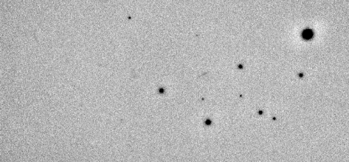
Figure 1: Image of our field centred at 3845Å. North is upwards and East to the left. The field is 500″ east-west and 235″ north-south. PKS 0424-131 is the bright source slightly below the centre of the field.

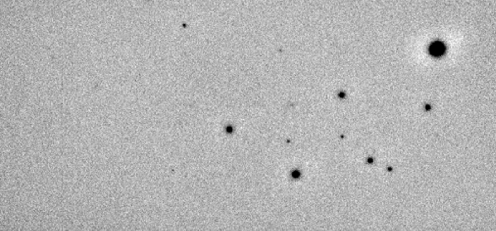
Figure 2: Image of our field centred at 3851Å. Details as in Fig 1.

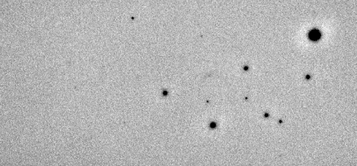
Figure 3: Image of our field centred at 3857Å. Details as in Fig 1.

No sources were found with excess flux in any of the narrow-band filters significant at the $5\sigma$ level, on any scale. Our $5\sigma$ sensitivity limit for unresolved ($<2$″) sources corresponds to a line flux of $9.6\times 10^{-18}{\rm erg\ cm}^{-2}{\rm s}^{-1}$. For sources larger than $3\times 3$″, our $5\sigma$ surface brightness limit is $1.6\times 10^{-18}{\rm erg\ cm}^{-2}{\rm s}^{-1}{\rm arcsec}^{-2}$. This drops to $4.7\times 10^{-19}{\rm erg\ cm}^{-2}{\rm s}^{-1}{\rm arcsec}^{-2}$ for sources larger than $10\times 10$″. Galactic absorption at this wavelength is $\sim 0.33$ mag (Schlegel, Finkbeiner & Davis, 1998).

4 Predicted Source Properties

The Ly$\alpha$ sources could be ionised by the quasar (externally ionised) or by UV sources within them (internally ionised). We consider these in turn.

4.1 Externally Ionised Hydrogen

4.1.1 Surface Brightness

How bright should the fluorescent Ly$\alpha$ emission from a neutral hydrogen cloud lying close to a bright QSO be? Let us approximate the spectrum of a QSO as a power-law, of the form $L_{\nu}=L_{0}(\nu/\nu_{0})^{\alpha}$ where $L_{\nu}$ is the luminosity per unit frequency, and $L_{0}$ is this luminosity at a particular frequency $\nu_{0}$. For PKS 0424-131, we measured a flux of $4.3\times 10^{-16}{\rm erg\ cm}^{-2}{\rm s}^{-1}$Å^-1 at a wavelength of 5000Å, which corresponds at this redshift to a luminosity of $5.5\times 10^{23}{\rm W\ Hz}^{-1}$ at rest-frame $6\times 10^{14}{\rm Hz}$ (correcting for Galactic extinction). This is very consistent with the various brightness measurements of this quasar in the literature: we see no evidence for variability. In the rest-frame far-UV, QSOs have $\alpha\sim-0.7$ (Francis et al., 1991). The number of ionizing photons emitted per unit time is thus:

$$N=L_{0}\int_{\nu_{LL}}^{\infty}\frac{1}{h\nu}\left(\frac{\nu}{\nu_{0}}\right)^{\alpha}d\nu=\frac{-L_{0}}{\alpha h}\left(\frac{\nu_{LL}}{\nu_{0}}\right)^{\alpha}$$ (1)

where $\nu_{LL}$ is the frequency of the Lyman limit ($3.29\times 10^{15}$ Hz).

Let us assume that this photon flux impacts face-on upon a plane-parallel cloud of neutral hydrogen, lying at a distance $r$ from the QSO. If the cloud is optically thick (typically $N_{H}>10^{17.2}{\rm cm}^{-2}$), all ionising photons will be absorbed. A fraction $\varepsilon$ will then be re-radiated as Ly$\alpha$ photons. Gould & Weinberg (1996) showed that $\varepsilon\sim 0.6$. The Ly$\alpha$ luminosity emitted by a neutral hydrogen cloud of area $A$ is thus:

$$L_{Ly\alpha}=\frac{\varepsilon}{4\pi r^{2}}\frac{L_{0}}{\alpha}\nu_{Ly\alpha}\left(\frac{\nu_{LL}}{\nu_{0}}\right)^{\alpha}$$ (2)

Given the observed brightness of PKS 0424-131, assuming $\alpha=-0.7$, $\varepsilon=0.6$, and that the cloud surface is orthogonal both to the quasar light and to our sight-line, the predicted surface brightness is thus:

$$1.2\times 10^{-18}\left(\frac{r}{1~{}{\rm Mpc}}\right)^{-2}{\rm erg\ cm}^{-2}{\rm s}^{-1}{\rm arcsec}^{-2}$$ (3)

Gas clouds whose surfaces are at an oblique angle to the incident photon flux will appear fainter, while those at an oblique angle to our line of sight will appear brighter: the two effects should cancel on average, but introduce a dispersion into the predicted surface brightnesses. We are ignoring radiative transfer within the cloud. The Ly$\alpha$ transition can have an enormous optical depth, but most of the clouds we will be seeing will be only marginally optically thick in the Lyman limit, so this effect may not be too severe. It will be severe for any damped Ly$\alpha$ systems lying near the QSO: we may only be able to see these if they lie on the far side of the QSO, so we are directly observing the illuminated face.

Given these predicted surface brightnesses, and our measured sensitivity limits, we should be able to detect neutral hydrogen clouds that subtend $1\times 1$″ (8.2 proper kpc) out to $r\sim 300$ kpc from the quasar. Larger clouds should be detectable at larger radii: clouds subtending $3\times 3$″ should be detectable out to $r\sim 740$ kpc while clouds subtending $10\times 10$″ should be detectable out to $r\sim 1350$ kpc.

4.1.2 Source Density

We are sampling a much smaller co-moving volume than most previous narrow-band Ly$\alpha$ surveys: is there a risk that we might not find anything in so small a volume?

QSO absorption-line statistics tell us the typical number of Lyman limit systems found per unit redshift along a QSO sight-line. Péroux et al. (2003) have compiled data from several surveys and give a number of Lyman-limit systems per unit redshift at z=2.16 of $N(z)=1.6$. In this section, we assume that the region close to the QSO is typical of the universe at this redshift (but see § 5.3).

Let us now assume that Lyman-limit systems are all face-on squares of side-length $r$. Consider a square region of the sky, of size $D\times D$, observed with a narrow-band filter sensitive to Ly$\alpha$ emission over a redshift range $\Delta z$. The probability of any given sight-line through this volume intersecting a Lyman-limit system is $P=N(z)\Delta z$. This should be equal to the fraction of the cross-sectional area of this region covered by the Lyman-limit systems; ie. $nr^{2}/D^{2}$, where $n$ is the number of Lyman-limit systems in the region, and $P\ll 1$. Thus:

$$n=N(z)\Delta z\left(\frac{D}{r}\right)^{2}$$ (4)

The 3D geometry of the region we survey (ignoring peculiar motions) is shown in Fig 4. Between our three central wavelength images, we fully sample a sphere around the QSO of radius 740 kpc (the radius to which we are sensitive to clouds subtending $3\times 3\arcsec$ or larger), and sample most of a sphere of radius 1430 kpc (in which we are sensitive to clouds subtending $10\times 10\arcsec$ or larger; § 4.1.1).

Figure 4: The 3D geometry of the volume in which we are sensitive to neutral hydrogen clouds. The solid lines show the volumes sampled by our three different central wavelength images. The dotted circles show the volumes out to which we should be able to find clouds subtending $1\times 1\arcsec$ (smallest circle), $3\times 3\arcsec$ and $10\times 10\arcsec$ (largest circle). 1000 Kpc equals two transverse arcminutes at this redshift. A cloud subtending $1\times 1\arcsec$ would be unresolved at our $1.8\arcsec$ seeing, which has been taken into account in computing the radius out to which it would be detectable.

Could we miss galaxies because of their peculiar motions in the potential well of a possible cluster surrounding PKS 0424-131? Between the three images we cover a velocity range of $\sim 1500{\rm km\ s}^{-1}$, so this should not be a problem unless there is a very massive cluster indeed. The existence of a cluster this massive at this redshift would be interesting in itself (eg. Rosati, Borgani & Norman, 2002). The $z=2.16$ cluster identified by Pentericci et al. (2000) had two sub-components, with velocity dispersions of $300$ and $500{\rm km\ s}^{-1}$, so either would easily fit within our passband.

Given this geometry, and our field of view (ample for all except the largest sphere), and making the same assumptions about neutral hydrogen cloud size as in § 4.1.1, we should have seen $\sim 20$ $1\times 1\arcsec$ clouds, $\sim 25$ $3\times 3\arcsec$ clouds, or around 6 $10\times 10\arcsec$ clouds. Only if the clouds were larger than 20 arcsec (160 kpc) would the expected number fall below one.

4.2 Internally Ionised Hydrogen

Many authors have shown that at sufficiently faint flux levels, a substantial population of Ly$\alpha$ emitting sources is seen at high redshift (eg. Cowie & Hu, 1998; Pascarelle et al., 1998; Kudritzki et al., 2000). As these sources are seen far from any QSOs, the ionisation must be generated locally, probably by weak AGNs or star formation within the galaxies.

We estimated how many of these sources we should see by comparing to the deepest existing Ly$\alpha$ surveys. The best match to our survey, both in redshift and depth, is that of Pascarelle et al. (1998). Their flux limit is very comparable to ours, and the co-moving volume they survey more than twice ours. Allowing for this difference, their results predict that we should see $\sim 6$ Ly$\alpha$ emitting sources. Kudritzki et al. (2000) surveyed a much larger volume at z=3.1, to a luminosity limit about four times brighter than ours. If we assume that the surface density of Ly$\alpha$ emitters increases by a factor of five for each magnitude we go deeper (Palunas et al., 2004), their results also predict that we should see $\sim 5$ sources. Similar numbers can be obtained by extrapolating from the results of Cowie & Hu (1998).

In practice, these numbers should be lower limits, as the region close to a luminous QSO is not a random part of the early universe. Work on high redshift radio galaxies has shown that they are surrounded by enhanced numbers of Ly$\alpha$ emitting sources (eg. Venemans et al., 2002, and references therein). Kurk et al. (2000) and Pentericci et al. (2000) searched for Ly$\alpha$ emitting sources around a radio galaxy at an almost identical redshift to our source, and down to a flux limit very comparable to our own. They found at least 14 Ly$\alpha$ emitting sources and a faint QSO, all within 1.5 projected Mpc of the radio galaxy. Comparable clusters of Ly$\alpha$ emitting galaxies are seen around other high redshift radio galaxies (eg. Le Fevre et al., 1996; Pascarelle et al., 1996; Venemans et al., 2002).

Could the Ly$\alpha$ emitters seen near these radio galaxies simply be neutral hydrogen clouds photoionised by UV from the AGN, rather than galaxies? While we see no UV from these radio galaxies, it may be emerging along an ionisation cone in some other direction. The Ly$\alpha$ sources are not, however, aligned in any particular area, or close to the radio jet axis, and the concealed nucleus would have to be far brighter in the UV than typical QSOs at this redshift. It therefore seems likely that these are indeed ionised internally.

We therefore conclude that we should have expected to see $\ga 10$ internally ionised Ly$\alpha$ emitting sources near our quasar, whereas we actually saw none.

5 Discussion: Why Didn’t We See Anything?

We showed in § 4.1 that if the region surrounding PKS 0424-131 were typical, we should have expected to have seen the fluorescent Ly$\alpha$ emission from a considerable number of clouds. We should also have seen internally ionised clouds. Instead, we saw nothing.

Could this just be a statistical fluke? Assuming Poisson statistics, the probability of seeing no sources given an expected number $n$ is $<1$% for $n>4$ and $<0.1$% for $n>6$. Our non-detection is thus reasonably significant, though clearly observations of several other luminous QSOs would be needed to test this. There have, however, been very few comparable observations. Campos et al. (1999) imaged a pair of QSOs at $z=2.58$, and found 37 candidate Ly$\alpha$ emitters, but they have no spectral confirmation, their QSOs are much fainter than ours, and they used a 130Å bandpass filter so the candidates may well lie at a somewhat different redshift to the QSOs. Hu & McMahon (1996) and Hu, McMahon & Egami (1996) found three luminous Ly$\alpha$ sources near two bright QSOs, but both QSOs lie at very different redshifts from ours ($z>4.5$). The only observations comparable to ours were those of Bergeron et al. (1999), who observed the $z=2.238$ QSO in the Hubble Deep Field South down to a flux limit about double ours. They found three candidate Ly$\alpha$ emitting sources, though their large (86 Å) bandpass means that they too may lie at a different redshift, and they have not published spectral confirmation of these sources. None of these QSOs have radio luminosities approaching that of PKS 0424-131.

We thus conclude that there is no compelling evidence in the literature for or against a deficit of faint Ly$\alpha$ emitters close to luminous, high redshift QSOs.

In this remainder of this section, we will assume that this deficit of Ly$\alpha$ emitters is a generic feature of extremely luminous QSOs at $z\sim 2$, and we will ask how such a deficit could be explained.

5.1 Lack of External Ionisation

How could we avoid the quasar PKS 0424-131 from ionising any neutral hydrogen clouds in its vicinity?

If it had only recently switched on its UV emission (at the time when the continuum radiation we see from it was being emitted), there may not have been time for this radiation to reach nearby gas clouds, ionise them and for the Ly$\alpha$ emission to reach the Earth. This would require that PKS 0424-131’s current active phase be younger than $\sim 10^{6}$ years. This is shorter than most estimates of the total lifespan of luminous QSOs (eg. Martini & Schneider, 2003, and refs therein). This total lifespan could, however, be divided up into several short active phases, or we could have been unlucky enough to have chosen a quasar very early in its active phase.

As noted in § 2.1 it is possible that PKS 0424-131 is a compact steep spectrum quasar. If this is the case, the upper limit on the size of the radio source (0.5″), combined with the typical expansion speed of jets (Bicknell, Saxton & Sutherland, 2003) allows us to place an upper limit on the age of the jet: $\sim 10^{5}$ years. If this radio source is beamed towards us, however, the size places no limit on the age. We plan Very Long Baseline Interferometry (VLBI) observations to discriminate between these two possibilities.

The calculations in § 4.1.2 assumed that the UV emission from PKS 0424-131 is isotropic. This is known not to be the case for many nearby Seyfert nuclei, where a “torus” intercepts $\sim 50$% of the ionising flux. If this were the case here, the expected numbers of externally ionised hydrogen clouds would be fewer than we predict. Note however that recent X-ray observations suggest that a smaller fraction of luminous QSO UV emission is blocked by tori at high redshifts (eg. Steffen et al., 2003). Observations of the transverse proximity effect in two sQSO (Liske & Williger, 2001; Jakobsen et al., 2003) provide further evidence that the UV radiation from high redshift escapes into substantial solid angles. Furthermore, we know from nearby Seyferts that up to 5% of the ionizing radiation field can be scattered almost isotropically by a warm nuclear wind (Miller, Goodrich & Mathews, 1991; Bland-Hawthorn, Sokolowski, & Cecil, 1991). This would render HI clouds visible over a 100 kpc sphere. Note however that, especially if the clouds are large, even a small reduction in the radius out to which we can see clouds, or even a narrow obscuring torus can drop the predicted number of clouds below 4, and hence drop the statistical significance of our null detection below 99%.

5.2 Absorption of the Ly$\alpha$ Emission

The Ly$\alpha$ line is the optically thickest transition in astrophysics, and hence is easily destroyed. If the ionised neutral hydrogen clouds are optically thick in Ly$\alpha$, their Ly$\alpha$ emission would only escape back towards the QSO. This would mean that we could only detect Ly$\alpha$ emission from clouds of the far side of the QSO. While this is likely to be true for any systems with $N_{H}\gg 10^{18}{\rm cm}^{-2}$ lying close to PKS 0424-131, we would expect many of the neutral hydrogen clouds to have lower optical depths, and hence be visible from all directions.

The high optical depth means that Ly$\alpha$ photons generated within a cloud will have to random-walk their way out. If any dust is present, this gives it multiple chances to absorb the Ly$\alpha$ photons. We know, however, that the Lyman-limit systems seen in absorption against bright QSOs contain very little dust: if they were dusty, the background QSO would have been too faint to observe. There may be a population of dusty absorbers, but they would be in addition to the population known from QSO absorption-line statistics (eg. Fall & Pei, 1993).

We also know that many high-redshift galaxies emit Ly$\alpha$, despite being ionised from the inside. Any Lyman-limit systems near the QSO would be ionised from the outside, enhancing the probability of any Ly$\alpha$ photons escaping.

We therefore tentatively conclude that the high optical depth of Ly$\alpha$ is unlikely to make all the hydrogen clouds in our field invisible. Even if it does render any externally ionised clouds undetectable, we should see at least the space density of internally ionised clouds found elsewhere in the high redshift universe.

5.3 Destruction of Hydrogen Clouds near the Quasar

This leaves us with the third possibility: that we see no Ly$\alpha$ emitters because there are no neutral hydrogen clouds close to the quasar.

If this very luminous QSO lies in a rich cluster environment, the surrounding gas might be heated to X-ray emitting temperatures, and the surrounding galaxies might be deficient in neutral hydrogen, by analogy with the traditional view of modern galaxy clusters (Giovanelli & Haynes, 1985; Cayatte et al., 1990). However, recent studies show that stripping in clusters today is much less effective than originally suggested. The most comprehensive survey to date, incorporating 1900 galaxies in 18 clusters (Solanes et al., 2001), finds that more than one-half of spiral galaxies retain at least half their HI within 900 $h_{70}^{-1}$ kpc. This is the scale, roughly 40% of an Abell radius, over which we expect to see disks with bright HI disks or halos. A third of the clusters in the Solanes et al. sample show no HI deficiency.

Furthermore, dense galaxy clusters are not thought to be common at such high redshifts (Rosati, Borgani & Norman, 2002). One would also expect high redshift radio galaxies to inhabit similar environments to our quasar, and as noted in § 4.2, overdensities of Ly$\alpha$ emitting sources are found around them. Other candidate high-redshift clusters also seem to have overdensities of Ly$\alpha$ emitters (eg. Steidel et al., 2000; Palunas et al., 2004; Francis & Williger, 2004).

Could a wind from the quasar have cleared its environment of neutral hydrogen, as suggested by Scannapieco & Oh (2004)? Adelberger et al. (2003) showed evidence for a similar effect around Lyman-break galaxies, though the reason for this effect is unclear (eg. Croft et al., 2002; Kollmeier et al., 2003; Bruscoli et al., 2003). We note however that the existing evidence points to an overdensity of neutral hydrogen near AGNs, not a deficit. Furthermore, such a wind could easily increase the brightness of any neutral hydrogen clouds by driving shocks into them (Francis et al., 2001).

The major difference between our quasar and the various high redshift radio galaxies is its enormous UV luminosity (at least along our line of sight). One possibility is that the quasar environment contains the normal quantity of hydrogen, but that this UV radiation has almost completely ionised it, so it is no longer optically thick in the Lyman-limit and is hence far less efficient at reprocessing the quasar flux into Ly$\alpha$ emission (the same effect that produces the proximity effect for Ly$\alpha$ forest clouds). We can compare the incident quasar flux at 912Å to the UV background flux at this wavelength ($\sim 7\times 10^{-22}{\rm erg\ cm}^{-2}{\rm Hz}^{-1}{\rm Sr}^{-1}$, Scott et al., 2002). Given the observed brightness of the QSO, assuming a typical QSO spectrum (Francis et al., 1991), and allowing for the fact that the UV background will impact both sides of a gas cloud while the quasar illuminates only one side, we find that at 1 Mpc from the quasar, its flux exceeds the UV background by a factor of $\sim 3$. At closer distances, where we would be seeing small clouds, the factor is much larger. Note that the ratio of fluxes at 912Å  underestimates the ratio of ionising flux as the UV background is more filtered by intervening material.

Given this enormous increase in ionising flux, how much might the number of optically thick externally ionised clouds decrease? We can crudely estimate this by assuming that if the incident ionising flux increased by a factor $x$, the cloud would need a hydrogen column density greater by the same factor $x$ to remaining optically thick. Péroux et al. (2003) showed that the cumulative number of QSO absorbers with hydrogen column densities greater than $N_{H}$ goes as $N_{H}^{-0.3}$. Using these figures, the number of externally ionised clouds should decrease by a factor of $\sim 2$: not enough to explain our non-detection. There is no easy way to estimate the size of this effect on internally ionised clouds.

The extremely strong UV emission from PKS 0424-131 could physically destroy dwarf galaxies in its vicinity, as described by Barkana & Loeb (1999), Benson et al. (2002) and references therein. This photoevaporation mechanism heats the gas in small dark matter halos so much that it becomes unbound. This destruction may have taken place at a much higher redshift, during the assembly of the very massive black hole we infer in this quasar. This mechanism has the advantage of explaining the absence of Ly$\alpha$ emitters around our UV bright source but not around radio galaxies, and could well destroy internally ionised Ly$\alpha$ sources, if they are dwarf galaxies residing in small dark matter halos.

6 Conclusions

Why then did we see nothing? There are several possible reasons which might explain the lack of externally ionised clouds, but the lack of internally ionised clouds is harder to explain. The difference between this UV-bright quasar and radio galaxies at comparable wavelengths points to the UV emission as a possible explanation. We therefore tentatively conclude that the UV photo-evaporation model seems the best explanation for our non-detection. With observations of only one QSO, however, this must be regarded as tentative at best.

How could we test this conclusion? Observations of more QSOs, and a better understanding of the background density of internally ionised Ly$\alpha$ sources at this redshift will clearly be vital to establishing whether this deficit of gas near luminous QSOs is real. With the recent decommissioning of TTF, this will have to be done at a different telescope.

If the sensitivity can be increased by a factor of $\sim 3$, we should be able to detect neutral hydrogen clouds ionised only by the UV background: ie. we can dispense with a nearby QSO. This should be quite feasible with long exposure times on an 8-10m class telescope. Alas most such telescopes do not have imagers capable of achieving the necessary spectral resolution, and most detectors have poor quantum efficiency in the UV. One exception will be the Osiris instrument, which incorporates many of the features of TTF, currently under construction for the Gran Telescopio Canarias (Cepa et al., 2003). Not only should this allow us to image neutral hydrogen clouds far from QSOs and hence measure their sizes and shapes, the anticipated sensitivity of this machine should allow many tens of QSO fields to be surveyed out to $z\sim 5$ over a range of intrinsic ionizing luminosities. This may be a relatively direct way to establish the critical ionizing flux at which star formation is effectively suppressed in the local universe.

References

- Adelberger et al. (2003) Adelberger, K.L., Steidel, C.C., Shapley, A.E. & Pettini, M. 2003, ApJ, 584, 45
- Aragon-Salamanca et al. (1994) Aragon-Salamanca, A., Ellis, R.S., Schwartzenberg, J.-M. & Bergeron, J.A. 1994, ApJ, 421, 27
- Barkana & Loeb (1999) Barkana, R. & Loeb, A. 1999, ApJ, 523, 54
- Barthel et al. (1988) Barthel, P.D., Miley, G.K., Schilizzi, R.T. & Lonsdale, C.J. 1988, A&A Suppl., 73, 515
- Benson et al. (2002) Benson, A.J., Lacey, C.G., Baugh, C.M., Cole, S. & Frenk, C.S. 2002, MNRAS, 333, 156
- Bergeron & Boissé (1991) Bergeron, J. & Boissé, P. 1991, A&A, 243, 344
- Bergeron et al. (1999) Bergeron, J., Petitjean, P., Cristiani, S., Arnouts, S., Bresolin, R. & Fasano, G. 1999, A&A, 343, L40
- Bertin & Arnouts (1996) Bertin, E. & Arnouts, S. 1996, A&AS, 117, 393
- Bicknell, Saxton & Sutherland (2003) Bicknell, G.V., Saxton, C.J. & Sutherland, R.S. 2003, PASA, 20, 102
- Bland-Hawthorn, Sokolowski, & Cecil (1991) Bland-Hawthorn, J., Sokolowski, J. & Cecil, G.N. 1991, ApJ, 375, 78
- Bland-Hawthorn & Jones (1998) Bland-Hawthorn, J. & Jones, D.H. 1998, PASA, 15, 44
- Bruscoli et al. (2003) Bruscoli, M., Ferrara, A., Marri, S., Schneider, R., Maselli, A., Rollinde, E. & Aracil, B. 2003, MNRAS 343, 41
- Bunker, Marleau & Graham (1998) Bunker, A.J., Marleau, F.R. & Graham, J.R., 1998, AJ, 116, 2086
- Campos et al. (1999) Campos, A., Yahil, A., Windhorst, R.A., Richards, E.A., Pascarelle, S., Impey, C. & Petry, C. 1999, ApJL, 511, L1
- Cayatte et al. (1990) Cayatte, V., Balkowski, C., van Gorkom, J. H., & Kotanyi, C. 1990, AJ, 100, 604
- Cepa et al. (2003) Cepa, J. et al. 2003, SPIE, 4841, 1739
- Chen et al. (2001) Chen, H.-W., Lanzetta, K.M., Webb, J.K. & Barcons, X.2001, ApJ, 559, 654
- Condon et al. (1998) Condon, J.J., Cotton, W.D., Greisen, E.W., Yin, Q.F., Perley, R.A., Taylor, G.B., & Broderick, J.J. 1998, AJ, 115, 1693
- Cowie & Hu (1998) Cowie, L.L. & Hu, E.M. 1998, AJ, 115, 1319
- Croft et al. (2002) Croft, R.A.C., Hernquist, L., Springel, V., Westover, M. & WHite, M. 2002, ApJ, 580, 634
- Crotts & Fang (1998) Crotts, A.P.S. & Fang, Y. 1998, ApJ, 502, 16
- Espey et al. (1989) Espey, B.R., Carswell, R.F., Bailey, J.A., Smith, M.G. & Ward, M.J. 1989, ApJ, 342, 666
- Fall & Pei (1993) Fall, S.M. & Pei, Y.C. 1993, ApJ, 402, 479
- Ferrarese (2002) Ferrarese, L. 2002, ApJ, 578, 90
- Foltz et al. (1984) Foltz, C.B., Weymann, R.J., Roser, H.-J. & Chaffee, F.H.Jr. 1984, ApJL, 281, 1
- Francis, Wilson & Woodgate (2001) Francis, P.J., Wilson, G.M. & Woodgate, B.E. 2001, PASA, 18, 64
- Francis & Hewett (1993) Francis, P.J. & Hewitt, P.C. 1993, AJ, 105, 1633
- Francis & Williger (2004) Francis, P.J. & Williger, G.M. 2004, ApJL, 602, L77
- Francis et al. (1991) Francis, P.J., Hewett, P.C., Foltz, C.B., Chaffee, F.H., Weymann, R.J. & Morris, S.L. 1991, ApJ, 373, 465
- Francis et al. (2001) Francis, P.J. et al. 2001, ApJ, 554, 1001
- Giovanelli & Haynes (1985) Giovanelli, R. & Haynes, M.P. 1985, ApJ, 292, 404
- Gould & Weinberg (1996) Gould, A. & Weinberg, D.H. 1996, ApJ, 468, 462
- Hogan & Weymann (1987) Hogan, C.J. & Weymann, R.J. 1987, MNRAS, 225, P1
- Haehnelt, Steinmetz & Rauch (1998) Haehnelt, M.G., Steinmetz, M.G. & Rauch, M. 1998, ApJ, 495, 647
- Haiman & Rees (2001) Haiman, Z. & Rees, M.J. 2001, ApJ, 468, 87
- Hu & McMahon (1996) Hu, E.M. & McMahon, R.G. 1996, Nature, 382, 231
- Hu, McMahon & Egami (1996) Hu, E.M., McMahon, R.G. & Egami, E. 1996, ApJL, 459, 53
- Hu et al. (2004) Hu, E.M., Cowie, L.L., Capak, P., McMahon, R.G., Hayashine, T. & Komiyami, Y. 2004, AJ, 127, 563
- Impey et al. (2002) Impey, C.D., Petry, C.E., Foltz, C.B., Hewett, P.C. & Chaffee, F.H. 2002, ApJ, 574, 623
- Jakobsen et al. (2003) Jakobsen, P., Jansen, R.A., Wagner, S. & Reimers, D. 2003, A&A, 397, 891
- Jones, Shopbell & Bland-Hawthorn (2002) Jones, D.H., Shopbell, P.L. & Bland-Hawthorn, J. 2002, MNRAS, 329, 759
- Kaspi et al. (2000) Kaspi, S., Smith, P.S., Netzer, H., Maoz, D., Jannuzi, B.T. & Giveon, U. 2000, ApJ, 533, 631
- Kollmeier et al. (2003) Kollmeier, J.A., Weinberg, D.H., Davé, R. & Katz, N. 2003, ApJ, 594, 75
- Kurk et al. (2000) Kurk, J.D., Röttgering, H.J.A., Pentericci, L., Miley, G.K., van Breugel, W., Carilli, C.L., Ford, H., Heckman, T., McCarthy, P. & Moorwood, A. 200, A&A, 358, L1
- Kudritzki et al. (2000) Kudritzki, R.-P., Méndez, R.H., Feldmeier, J.J., Ciardullo, R., Jackoby, G.H., Freeman, K.C., Arnaboldi, M., Capaccioli, M., Gerhard, O. & Ford, H.C. 2000, ApJ, 536, 19
- Le Fevre et al. (1996) Le Fevre, O., Deltorn, J.M., Crampton, D. & Dickinson, M. 1996, ApJL, 471, L11
- Liske & Williger (2001) Liske, J. & Williger, G.M. 2001, MNRAS, 328, 353
- Maloney & Bland-Hawthorn (2001) Maloney, P.R. & Bland-Hawthorn, J. 2001, ApJ, 553, L129
- Martini & Schneider (2003) Martini, P. & Schneider, D.P. 2003, ApJL, 597, L109
- McIntosh et al. (1999) McIntosh, D.H., Rieke, M.J., Rix, H.-W., Foltz, C.B. & Weymann, R.J. 1999, ApJ, 514, 40
- Miller, Goodrich & Mathews (1991) Miller, J.S., Goodrich, R.W. & Mathews, W.G. 1991, ApJ, 378, 47
- Møller & Warren (1993) Møller, P. & Warren, S.J. 1993, A&A, 270, 43
- Møller et al. (2002) Møller, P., Warren, S.J., Fall, S.M., Fynbo, J.U. & Jakobsen, P. 2002, ApJ, 574, 51
- Ouchi et al. (2003) Ouchi, M. et al. 2003, ApJ, 582, 60
- Palunas et al. (2004) Palunas, P., Teplitz, H.I., Francis, P.J., Williger, G.M. & Woodgate, B.E. 2004, ApJ, 602, 545
- Pascarelle et al. (1996) Pascarelle, S.M., Windhorst, R.A., Driver, S.P., Ostrander, E.J. & Keel, W.C. 1996, ApJL, 456, L21
- Pascarelle et al. (1998) Pascarelle, S.M., Windhorst, R.A. & Keel, W.C. 1998, AJ, 116, 2656
- Pentericci et al. (2000) Pentericci, L., Kurk, J.D., Röttgering, H.J.A., Miley, G.K., van Breugel, W., Carilli, C.L., Ford, H., Heckman, T., McCarthy, P. & Moorwood, A. 2000, A&A, 361, 25
- Pei, Fall & Hauser (1999) Pei, Y.C., Fall, S.M. & Hauser, M.G. 1999, ApJ, 522, 604
- Péroux et al. (2003) Péroux, C., McMahon, R.G., Storrie-Lombardi, L.J. & Irwin, M.J. 2003, MNRAS, 346, 1103
- Petitjean, Rauch & Carswell (1994) Petitjean, P., Rauch, M. & Carswell, R.F. 1994, A&A, 291, 29
- Prochaska & Wolfe (1998) Prochaska, J. & Wolfe, A. 1998, ApJ, 507, 113
- Rauch, Sargent & Barlow (1999) Rauch, M., Sargent, W.L.W. & Barlow, T.A. 1999, ApJ, 515, 500
- Rosati, Borgani & Norman (2002) Rosati, P., Borgani, S. & Norman, C. 2002, ARAA, 40, 539
- Scannapieco & Oh (2004) Scannapieco, E. & Oh, S.P. 2004, ApJ submitted (astro-ph/0401087)
- Schlegel, Finkbeiner & Davis (1998) Schlegel, D.J., Finkbeiner, D.P. & Davis, M. ApJ, 500, 525
- Scott et al. (2002) Scott, J., Bechtold, J., Morita, M., Dobrzycki, A. & Kulkarni, V.P. 2002, ApJ, 571, 665
- Smette et al. (1995) Smette, A., Robertson, J.G., Shaver, P.A., Reimers, D., Wisotzki, L. & Koehler, T. 1995, A&A 113, 199
- Solanes et al. (2001) Solanes, J. M., Manrique, A., Garc a-G mez, C., Gonz lez-Casado, G., Giovanelli, R., & Haynes, M. P. 2001, ApJ, 548, 97
- Steffen et al. (2003) Steffen, A.T., Barger, A.J., Cowie, L.L., Mushotzky, R.F. & Yang, Y. 2003, ApJL, 596, L23
- Steidel et al. (2000) Steidel, C.C., Adelberger, K.L., Shapley, A.E., Pettini, M., Dickinson, M. & Giavalisco, M. 2000, ApJ, 532, 170
- Steidel et al. (2002) Steidel, C.C., Kollmeier, J.A., Shapley, A.E., Churchill, C.W., Dickinson, M. & Pettini, M. 2002, ApJ, 570, 526
- Venemans et al. (2002) Venemans, B.P., Kurk, J.D., Miley, G.K., Röttgering, H.J.A., van Breugel, W., Carilli, C.L., Ford, H., Heckman, T., McCarthy, & Pentericci, L., 2002, A&A, 361, 25