Distribution of Singularities in the Cosmic Microwave Background Polarization

Abstract

The polarization of the cosmic microwave background radiation will have a distribution of singularities and anti-singularities, points where the polarization vanishes for topological reasons. The statistics of polarization singularities provides a non-trivial scheme to analyze the polarization maps that is distinct from the usual two-point correlation functions. Here we characterize the statistics of the singularity distribution in simulated polarization maps, and make predictions that can be compared with ongoing and upcoming observations. We use three different characterizations: the nearest neighbor distance between singularities, the critical exponent $\nu$ that captures the scaling of total charge $q$ within a closed curve of length $L$ ($q\propto L^{\nu}$), and the angular two point angular correlation functions for singularities of similar and opposite charge. In general, we find that the distribution of singularities is random except on scales less than about $10^{\circ}$, where singularities of the same charge repel and those of opposite charge attract. These conclusions appear to be extremely robust with respect to variations in the underlying cosmological model and the presence of non-Gaussianity; the only exception we found are cases where statistical isotropy is grossly violated. This suggests that, within the assumption of statistical isotropy, the distribution is a robust feature of the last scattering surface and potentially may be used as a tool to discriminate effects that occur during photon propagation from the last scattering surface to the present epoch.

The cosmic microwave background (CMB) anisotropies are linearly polarized at the 10% level. The polarization, predicted almost four decades ago rees , has recently been observed dasi ; wmap_pol and efforts are underway to map it on increasingly smaller scales. The polarization is most easily described in terms of so-called E and B modes KamKosSte97 ; SeljZal_EB . The two-point correlation function of E and B maps is typically taken as a statistic of choice to represent the polarization properties of the map. The two-point function fully describes the map if it is Gaussian random and isotropic, otherwise higher-order correlation functions are necessary for the full description (for a review of CMB polarization, see e.g. Ref. hu_white ).

In this paper we explore another, independent and largely unexplored signature of CMB polarization: the distribution of singularities NasNov98 ; dolgov ; VacLue03 . The CMB polarization map (denoted $P$) corresponds to a map from the sky – the two dimensional sphere, $S^{2}$ – to the space of headless vectors, $S^{2}/Z_{2}$, given by the plane and amplitude of polarization:

$$P:S^{2}\rightarrow S^{2}/Z_{2}$$ (1)

Such maps are known to contain topological features that are characterized by points with vanishing polarization, known as “singularities” or “defects”, and each singularity carries a topological charge. The total topological charge within a closed contour on the sky can be calculated as an integral over the contour. This is very similar to Gauss’ law that is used to determine the electric charge within a closed surface by integrating the electric field over the surface. The polarization singularities have fundamental charge $+1/2$. The anti-singularities have fundamental charge $-1/2$. These fundamental singularities are shown in Fig. 1. They can be combined to form three kinds of double singularities as shown in Fig. 2: “knots” and “foci”, which have charge $+1$, and “saddles” with charge $-1$ NasNov98 . The total charge in a given map is zero for all practical purposes, as discussed in the next Section.

Figure 1: Fundamental singularities of charge $\pm 1/2$. Each dash represents the linear polarization of the CMB radiation at that point. The $\times$ marks the position of the singularity where the linear polarization vanishes for topological reasons.

Figure 2: Singularities of charge $\pm 1$, constructed by combining the two fundamental singularities shown in Fig. 1. Top row shows examples of a “knot” and a “focus”, while a “saddle” is shown at the bottom, using the nomenclature from Ref. NasNov98 .

Polarization of the CMB, like the temperature, provides an extremely important window to the processes in the early universe. In fact, the polarization has some advantages over the temperature, and in particular it offers a more direct probe of the recombination era at large angular scales hu_okamoto . It is therefore well worthwhile to consider alternative analyses of the polarization, and this motivates us to explore the distribution of singularities. Our predictions can be tested as soon as polarization maps become available. Furthermore, since all of our statistics are computed in real (and not Fourier) space, sky cuts due to galaxy and other foreground contamination will be relatively easy to take into account.

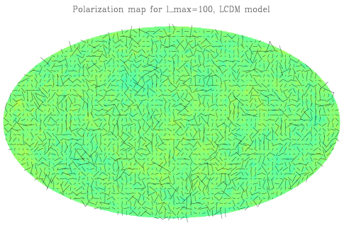
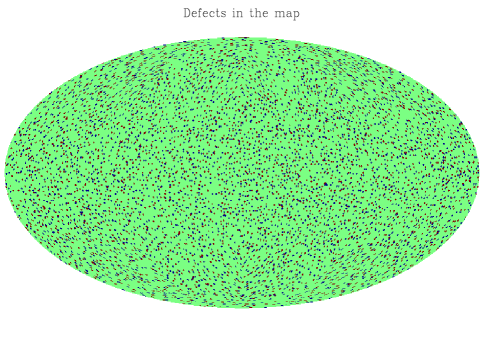
Figure 3: Left panel: An example of the mock polarization map. For visual clarity, this map was produced at the resolution NSIDE$=256$, has power out to $\ell_{\rm max}=50$ and contains about 6000 singularities. Right panel: The distribution of singularities in the same map.

Polarization singularities have first been described in Refs. NasNov98 and dolgov . The expected distribution has been described in Ref. VacLue03 based on earlier experience with condensed matter systems. We extend previous work and use a highly quantitative analysis of the singularities, describe their statistic as a function of pixelization scale and the underlying cosmological model, and assess the statistical errors for each measurement.

I The definition of singularities

The polarization patterns with fundamental (charge $\pm 1/2$) singularities are shown in Fig. 1. The polarization map is described by the Stokes parameters $Q$ and $U$. The properties of the polarization under rotations imply that:

$$Q=I\cos(2\alpha)\ ,\ \ U=I\sin(2\alpha)$$ (2)

where $I$ is the radiation intensity and $\alpha$ is the polarization angle. The $\pm 1/2$ singularities are locations around which $\alpha$ changes by $\pm\pi$. Therefore, given a polarization map, we can find the change in $\alpha$ as we go around a small closed path and this will tell us whether there is a singularity within that closed path. By going around all possible paths, we can find all the polarization singularities. In the continuum, there would be an infinite number of small paths. But in practice, the map is pixelized and the change in $\alpha$ is found around circuits defined by neighboring pixels. The algorithm for finding the singularities in a pixelated map is well-known and is described in the Appendix.

In this paper we will be concerned with the distribution of polarization singularities. We will characterize the distribution in three distinct ways. The first method is to find the total charge $q$ within a closed path of length $L$. The mean charge will, of course, be zero because one can have positive and negative charges with equal probability . Next, we compute the distribution of the distance to the nearest neighbor of a singularity. Finally, motivated by the analyses of the galaxy distribution on the sky, we compute the angular two-point correlation function of singularities in the polarization map. This work complements the pioneering theoretical discussions in Refs. NasNov98 ; dolgov ; VacLue03 and helps establish the distribution of singularities in the CMB polarization as a significant probe of the universe.

In the next section, we describe how we create the mock polarization maps. In Sec. III we find the critical exponents and the angular correlation function, as well as the distribution of distance to the nearest neighbor for a vanilla mock map. We investigate the effects of non-random phases and non-Gaussianity in Sec. IV and summarize our results in Sec. V. In the Appendix we describe the algorithm for determining the presence of a singularity.

II Scheme to produce mock polarization maps

To produce mock polarization maps, we proceed as follows. We first produce the angular power spectra (temperature and polarization) of the CMB using the CMBFAST package cmbfast . Our fiducial model is the standard $\Lambda$CDM cosmology with a flat universe with matter energy density relative to critical $\Omega_{M}=0.3$, dark energy equation of state $w=-1$, scalar spectral index $n_{s}=1.0$, physical matter and baryon energy densities of $\Omega_{M}h^{2}=0.127$ and $\Omega_{B}h^{2}=0.021$ respectively, and no tensor modes (we explore the variations to this model in Sec. IV). We can obtain an arbitrary number of statistically independent maps by generating different sets of coefficients $a_{\ell m}^{E}$ and $a_{\ell m}^{B}$, consistent with the same underlying power spectra $C_{\ell}^{E}$ and $C_{\ell}^{B}$ respectively, and generating the polarization map in Healpix healpix for each set separately. Recall that the coefficients $a_{\ell m}^{(E,B)}$ fully describe a given map and, for a Gaussian random map, come from a Gaussian distribution of variance $C_{\ell}^{(E,B)}$. In some cases we will want to produce polarization maps that do not come from Gaussian random $a_{\ell m}$, and in those cases we simply input the desired non-Gaussian $a_{\ell m}^{(E,B)}$ directly.

III Statistics of the Singularity Distribution

III.1 Number of singularities

We first compute the total number of singularities (or charges) $N_{\rm sin}$, positive plus negative, in a given mock map. As expected, the number of charges increases with the map resolution, just as, for example, the number of temperature hot and cold spots increases with resolution. $N_{\rm sin}$ increases roughly as the square of the maximum resolution of the map $\ell_{\rm max}$ so that, for example, a map (consistent with our fiducial $\Lambda$CDM model) with $\ell_{\rm max}=100$ has about 6000 singularities, while a map with $\ell_{\rm max}=500$ has about 150,000 singularities. Note that, even if we are able to measure the polarization with infinite resolution, $N_{\rm sin}$ does not increase indefinitely, but levels off when the power in polarization becomes negligible. For a standard $\Lambda$CDM model, the EE power spectrum has power all the way to $\ell\sim 2000$. However, this implies that the total number of singularities is likely to be larger than a million, making the analysis of such a map challenging. Fortunately, we do not need to worry about this issue, or wait for polarization experiments that will reach scales this small, such as PLANCK, in order to explore the distribution of singularities: the tests we propose can be performed for polarization maps covering any range of angular scales, and statistics from the measured map of any given resolution can be compared to Monte Carlo tests with mock maps of the same resolution.

III.2 Scaling of RMS charge

We would now like to quantify how the variance in the number of singularities increases with the area covered on any given map. The root-mean-square (RMS) fluctuation of the charge within a closed path of length $L$ is expected to be:

$$\sigma(q(L))\equiv\left<\left(q(L)-\bar{q}(L)\right)^{2}\right>^{1/2}=aL^{\nu}$$ (3)

where $q(L)$ is the total (positive plus negative) charge within $L$, $\bar{q}(L)$ is its mean among the different paths of the same length, $a$ is a system-dependent constant and the critical exponent $\nu$ is expected to be 0.5 VacLue03 . Using our numerical analysis of mock data we will be able to predict both $a$ and $\nu$ together with error bars.

To compute the RMS of charge per ring, we create a polarization map, and pick a point on it that we call the North Pole. In the Healpix representation of the map, each ring of angle $\theta$ from the North Pole has length $L=2\pi\sin{\theta}$, and we find $q(L)$ for all rings using the procedure described in the Appendix. We then rotate the north pole of the map in a random direction (i.e. assign it to a new, randomly chosen point on the sphere) and repeat the computation of $q(L)$ for each ring. We repeat this procedure hundred times in order to obtain sufficient statistics and compute $\sigma(q(L))$. The mean charge per ring, averaged over all rotations, is nearly zero, while the fluctuations around the mean is what we are interested in.

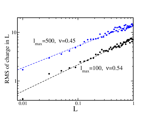
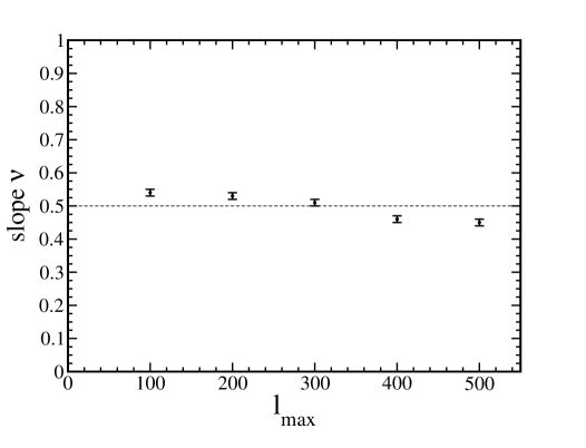
Figure 4: Top panel: Root-mean-square of the total charge per ring as a function of the ring’s length $L$. The two datasets correspond to polarization maps with resolution $\ell_{\rm max}=100$ (bottom) and $\ell_{\rm max}=500$ (top), while the dashed curves denote the linear fit in the log-log coordinates. The distributions are consistent with $\sigma(q(L))\propto L^{\nu}$ with $0.45\lesssim\nu\lesssim 0.55$. Bottom panel: the dependence of $\nu$ on the maximum resolution of the map $\ell_{\rm max}$ ($\ell_{\rm max}$ is the maximum multipole where the map has power).

Figure 4 (top panel) shows the scaling of $\sigma(q(L))$ with $L$ for maps of two resolutions $\ell_{\rm max}=100$ and $500$, corresponding to polarization having power down to scales of $\sim 1^{\circ}$ and $\sim 0.4^{\circ}$ respectively. In both cases we have fixed the pixelization of the map to the Healpix parameter NSIDE$=256$, corresponding to pixels of about $0.25^{\circ}$ on a side. In these and many other cases we have explored, the RMS of charge scales as $L^{\nu}$ where the critical exponent $\nu$ is nearly 0.5, in agreement with expectations. Furthermore, the exponent is independent of the map pixelization NSIDE. However, we find that the exponent slightly decreases with map resolution, moving from $\approx 0.55$ for $\ell_{\rm max}=100$ to $\approx 0.45$ for $\ell_{\rm max}=500$; see the bottom panel of Fig. 4. In all cases the error in the exponent is about $0.01$.

III.3 Distance to the nearest neighbor

Another statistic that we explore is the distance to the nearest neighbor from any given singularity. The histogram of the distances to the nearest neighbor is shown in Fig. 5, where for computational convenience we have assumed a map with $\ell_{\rm max}=100$ which has a total of about $6000$ singularities. The average distance to the nearest neighbor is slightly above $2^{\circ}$ and can be roughly predicted from the total number of singularities ($\sim 6000$ singularities in $\sim 40000$ degrees on the sky). However, the histograms of the nearest neighbor of the same charge and that of the opposite charge are different, and show that opposite charges attract and similar charges repel. For example, the mean distance to the nearest neighbor of the same charge is $(3.24\pm 0.01)^{\circ}$, while distance to the neighbor of the opposite charge is $(2.69\pm 0.01)^{\circ}$.

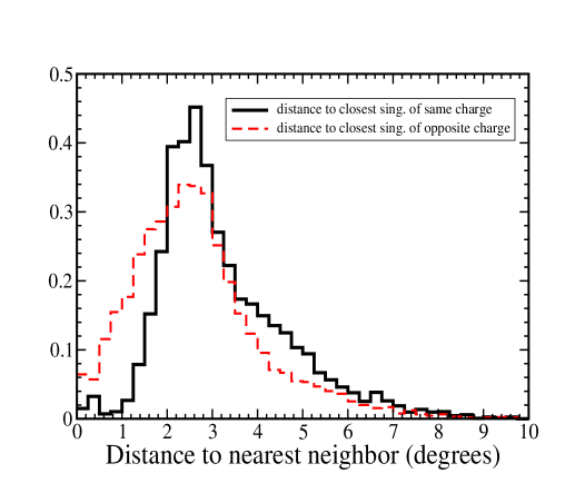
Figure 5: Histogram of the distance from any given singularity to the nearest neighbor of the same charge (black-solid) and opposite charge (red-dashed). Note the effects of repulsion between charges of the same sign, and attraction of charges of the opposite sign.

III.4 Angular power spectrum of singularities

The third characterization of the singularity distribution we suggest and explore is the two point angular correlation function $w(\theta)$. The angular two point function is simply the excess probability, on top of expectation due to random distribution, of finding one singularity at an angular location ${\vec{\theta}}_{1}$ and another one at location ${\vec{\theta}}_{2}$

$$dP(\vec{\theta}_{1},\vec{\theta}_{2}) = dP(\vec{\theta}_{1})\,dP(\vec{\theta}_{2})\,(1+w(\vec{\theta}_{1}-\vec{\theta_{2}}))$$ (4)

$$= dP(\vec{\theta}_{1})\,dP(\vec{\theta}_{2})\,(1+w(\theta))$$ (5)

where $\theta=|\,\vec{\theta}_{1}-\vec{\theta_{2}}|$ and the second line assumes statistical isotropy. In addition to the angular correlation function for all singularities, we can find individual $w(\theta)$ for singularities of positive (or negative) charge in a similar way.

The angular correlation function is one of the standard tools to describe the angular clustering of galaxies, and has been thoroughly explored and used during the past three decades. Computing $w(\theta)$ for the galaxy distribution, however, typically involves various practical problems, most important of which is the “selection function” of the survey, having to do with magnitude cuts and imperfect coverage across the field of view. The application we are considering here is vastly simpler, since the singularities are discrete, well-defined and easily computable features, and unlike the galaxies they are located at the same radial distance. Furthermore, we are simulating the polarization pattern on full skies and do not need to worry about edge-effects due to incomplete sky coverage. Therefore, a simple estimator for $w(\theta)$ will suffice. We adopt the Peebles-Hauser PeeHau estimator

$$w(\theta)={N_{\rm rand}\over N_{\rm map}}\left({DD(\theta)\over RR(\theta)}-1\right)$$ (6)

where $DD(\theta)$ is the number of singularity pairs separated by a distance larger than $\theta-d\theta$ but smaller than $\theta+d\theta$, $RR(\theta)$ is the number of pairs from a random (Poisson-distributed) map being in the same distance interval, and $N_{\rm map}$ and $N_{\rm rand}$ are the total numbers of singularities in the two maps. In other words, the angular correlation function measures the excess clustering over that predicted by random distribution on any given scale. Here we use $d\theta=5^{\circ}$, which is larger than our pixelization scale and thus avoids any edge-effects due to pixelization. We have tried several other values of $d\theta$ and obtained consistent results.

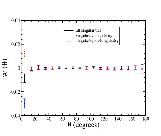
Figure 6: Angular correlation function of the distribution of singularities, showing the excess probability of clustering over that predicted by the random distribution. The overall distribution of singularities is consistent with random, except at small scales ($\lesssim 10^{\circ}$) where singularities of opposite charge attract while those of equal charge repel.

Figure 6 shows the angular two-point correlation function for the map with $\ell_{\rm max}=100$. In each case we compute $w(\theta)$ for 10 statistically independent maps, and plot the mean and standard deviation of measurements at all angular scales. Note that this procedure correctly accounts for the increase in the error bars at large angular separations due to sample (or cosmic) variance.

We find that $w(\theta)$ is remarkably consistent with zero at all angular scales greater than about $10^{\circ}$! This implies that the singularities are Poisson distributed over most angular scales. Also note that the singularity-singularity $w(\theta)$ is negative at scales $\lesssim 10^{\circ}$, while the singularity-antisingularity $w(\theta)$ is positive over the same range. This illustrates the fact we discussed in Sec. III.3, that charges of the same sign repel and those of opposite sign attract. Finally, $w(\theta)$ for all singularities (irrespective of their charge) shows an overall decrease at $\theta\lesssim 10^{\circ}$. We have repeated this analysis by varying the maximum resolution of the map $\ell_{\rm max}$ and found consistent results: the behavior of $w(\theta)$ is qualitatively similar, while the error bars decrease with increasing $\ell_{\rm max}$ due to the increase in the number of singularities.

IV Exploring departures from the standard cosmological model

It is important to determine how the singularity distribution depends on the physical input such as the primordial fluctuation spectrum, the cosmological parameters, or Gaussianity of cosmological seed perturbations. In particular, previous work NasNov98 ; dolgov emphasized that the distribution and type of singularities may be a promising way of probing the Gaussianity of initial conditions.

With this in mind we have created mock maps of the CMB polarization using several different cosmological models and characterized the singularity distribution in each. In particular, we have tried several extreme possibilities, some of which are already ruled out by cosmological observations:

• Maps based on primordial power spectrum with very significant tensor modes (the ratio of tensor to scalar perturbations at the CMB temperature quadrupole of $T/S=10$).

• Maps with a strongly tilted primordial power spectrum with either less or more power on small scales: we alternatively assumed a scalar spectral index $n_{s}=0$ or $n_{s}=2$.

• Maps that are strongly non-Gaussian: we assumed the real and imaginary parts of the coefficients $a_{\ell m}^{(E,B)}$ to be sampled from an exponential distribution while keeping zero mean and variance equal to $C_{\ell}^{(E,B)}/2$. In other words, we have adopted a highly skewed distribution of the coefficients $a_{\ell m}^{(E,B)}$.

Remarkably we find that all statistics we considered are largely unaffected. The critical exponent is unchanged within the errors, and so is its dependence on $\ell_{\rm max}$. The two point correlation function $w(\theta)$ is also unchanged, being consistent with zero except on scales less than $10^{\circ}$. The total number of singularities does change for the alternative cosmological models, which is to be expected since the total power in the map is affected each time. However, statistics of the distribution of singularities are unchanged.

In particular, we find it very interesting that the results are insensitive to the model for non-Gaussianity we assumed. We have explored this further for several other classes of variations to the standard Gaussian/isotropic assumption, and found deviations from the results described in Sec. III only in cases where the statistics of the map were modified enough that the statistical isotropy was grossly violated. For example, maps where the only nonzero $a_{\ell m}^{(E,B)}$ coefficients were those with $m=0$ showed deviation from results in Sec. III; however, inspection of polarization maps in these cases indicate that such modifications lead to huge violations of isotropy in the map that are easily detectable with almost any reasonable statistical test. Conversely, more subtle modifications of the power spectra (for example, setting the quadrupole of temperature and polarization to zero) produced the same results as our fiducial model. Therefore the characteristics of the singularity distribution seem to be robust features that are insensitive to the cosmological inputs at the last scattering surface.

The robustness of the singularity distribution holds advantages as well as disadvantages. One disadvantage is that by examining the distribution of the singularities in the actual data, it is unlikely that we will uncover something about the physics of the primordial fluctuations (unless statistical isotropy is violated). The advantage is that since the distribution is robust, any distortions in it must come during propagation of the photons from the last scattering surface to us. Hence the distribution can be used as a probe of cosmology at redshifts smaller than $1000$. For example, weak gravitational lensing could distort the Poissonian nature of the angular correlation functions; however, this effect will operate only at small angular scales, as lensing distortions are typically a few arcminutes.

V Conclusions

We have explored the statistics of the distribution of singularities in the CMB polarization maps. The existence of singularities are a generic prediction for a headless vector field on a sphere. Their distribution, however, has not been explored in the past except for some generic scaling arguments. Here we have provided a quantitative analysis of the distribution of singularities with positive and negative charge, and argued that the singularities provide an additional probe of the conditions at last scattering, largely independent of the usual two-point correlation functions of temperature.

We found that the singularities are distributed randomly at scales $\gtrsim 10^{\circ}$. The angular two-point correlation function of singularities vanishes at those scales, while the total charge within a closed path of length $L$ scales as $L^{\nu}$ with $\nu\simeq 0.5$. On scales $\lesssim 10^{\circ}$, however, charges of the same sign repel while those of opposite charge attract. The attraction and repulsion are manifested both in the angular two-point correlation function and in the distribution of the nearest-neighbor distance.

Perhaps surprisingly, we found that the aforementioned results are very robust with respect to variations in the underlying cosmological model assumed to create the mock maps. Changes in the tensor to scalar ratio, scalar spectral index, and non-Gaussian distributions of the $a_{lm}$’s all leave the singularity distribution unchanged. Only violations of statistical isotropy affected the distribution of singularities. It is still possible that there are some other forms of non-Gaussianity that can affect the singularity distribution that we have not explored. While this is impossible to rule out, it seems more likely to us that the distribution of singularities at the last scattering surface is described precisely by the Poissonian distribution and other characteristics we have found. This implies that any observed deviations of the actual map from these distributions will have to be due to line of sight effects. Most importantly, gravitational lensing of the CMB by the large-scale structure can cause changes in the singularity distribution. However, the lensing operates mostly on small scales, with typical deflections of a few arcminutes and coherence of $<10^{\circ}$. Therefore, lensing may affect the statistics of the singularity distribution only at small scales. We hope to explore this signature in future work.

Appendix A Calculation of the winding number

Here we will describe how the winding of polarization around a contour $\Gamma$, i.e. net topological charge within $\Gamma$, is calculated.

The polarization map specifies $Q(\theta,\phi)$ and $U(\theta,\phi)$, where $\theta$ and $\phi$ are galactic latitude and longitude. From $Q$ and $U$ we can determine the polarization angle $\alpha$:

$$\alpha(\theta,\phi)=\frac{1}{2}{\tan}^{-1}\biggl{(}\frac{U}{Q}\biggr{)}$$ (7)

Now we want to know the change in $\alpha$ as we go around the closed contour $\Gamma$.

Any map of the CMB polarization will be pixelized. Hence only an average value of $\alpha$ within each pixel will be available to us. Then the change in $\alpha$ in going from pixel $i$ to a neighboring pixel $i+1$ is given by:

$$\delta\alpha_{i}=\alpha_{i+1}-\alpha_{i}+\beta$$ (8)

where $\beta$ is defined as follows:

$$\beta=0\ ,\ \ \ {\rm if}\ |\alpha_{i+1}-\alpha_{i}|\leq\pi/2$$ (9)

$$\beta=+\pi\ ,\ \ \ {\rm if}\ \alpha_{i+1}-\alpha_{i}<-\pi/2$$ (10)

$$\beta=-\pi\ ,\ \ \ {\rm if}\ \alpha_{i+1}-\alpha_{i}>+\pi/2$$ (11)

In other words $\delta\alpha$ is the shortest path from $\alpha_{i}$ to $\alpha_{i+1}$ around the circle defined by $\alpha\in[-\pi/2,+\pi/2]$ (see Fig. 7). Note that $\alpha=-\pi/2$ yields the same $Q$ and $U$ as $\alpha=+\pi/2$ and hence these two points are identified.

Figure 7: To calculate the topological winding along a contour $\Gamma$ – here shown as a hexagon – we follow the phase $\alpha$, always choosing the shortest path on the $\alpha$ circle. $\alpha_{i}$ denotes the value of the phase at point $i$ on $\Gamma$. The net change in $\alpha/2\pi$ as $\Gamma$ is traversed is the winding. In the figure, the change in $\alpha$ is $-\pi$ since we go around the $\alpha$ circle once in the counter-clockwise direction. Note that the full circle in $\alpha$ corresponds to an angle of only $\pi$, not $2\pi$. Hence the topological charge within $\Gamma$ in the drawn example is $-1/2$.

The winding, $\Delta\alpha$, around the contour $\Gamma$ is now simply:

$$\Delta\alpha=\sum_{i}\delta\alpha_{i}$$ (12)

where the sum is over all the discretized steps that define $\Gamma$. The resulting topological charge is then $\Delta\alpha/(2\pi)$.

This scheme to find the windings has one small modification since the sky is $S^{2}$. In this case, since the polarization angle $\alpha$ is defined with respect to the lines of latitude and this definition breaks down at the North and South poles, we need to modify the scheme for any contour that contains the North (or the South) pole. In that case, 1 must be added (per enclosed pole) to the net topological charge within the contour. This also ensures that the total topological charge on the sky is $+2$ VacLue03 .

References

- (1) M.J. Rees, Astrophys. J. 153, L1 (1968)
- (2) J. Kovac et al., Nature 420, 772 (2002).
- (3) A. Kogut et al., Astrophys. J. Suppl. 148, 161 (2003).
- (4) M. Kamionkowski, A. Kosowsky, and A. Stebbins, Phys. Rev. D55, 7368 (1997).
- (5) U. Seljak and M. Zaldarriaga, Phys. Rev. D55, 1830 (1997).
- (6) W. Hu and M. White, New Astronomy 2, 323 (1997).
- (7) P.D. Naselsky and D. I. Novikov, Astrophys. J. 507, 31 (1998).
- (8) A. Dolgov, A. Doroshkevich, D. I. Novikov and I. D. Novikov, JETP Lett. 69, 427, (1999); A. Dolgov, A. Doroshkevich, D. Novikov and I. Novikov, Int. J. Mod. Phys. D8, 189 (1999).
- (9) T. Vachaspati and A. Lue, Phys. Rev. D67, 121302(R) (2003).
- (10) W. Hu and T. Okamoto, Phys. Rev. D 69, 043004 (2004).
- (11) U. Seljak and M. Zaldarriaga, Astrophys. J. 469, 437 (1996).
- (12) K. Gorski, E. Hivon and B.D. Wandelt, Proceedings of the MPA/ESO Cosmology Conference ”Evolution of Large-Scale Structure”, eds. A.J. Banday, R.S. Sheth and L. Da Costa, PrintPartners Ipskamp, NL, pp. 37-42 (astro-ph/9812350)
- (13) P.J.E. Peebles and M.G. Hauser, Astrophys. J. Suppl. 28, 19 (1974).