The Metal Content of the Bulge Globular Cluster NGC 6528

High resolution spectra of five stars in the bulge globular cluster NGC 6528 were obtained at the 8m VLT UT2-Kueyen telescope with the UVES spectrograph. Out of the five stars, two of them showed evidence of binarity. The target stars belong to the horizontal and red giant branch stages, at 4000 $<$ T_eff $<$ 4800 K. Multiband $V,I,J,H,K_{\rm s}$ photometry was used to derive initial effective temperatures and gravities. The main purpose of this study is the determination of metallicity and elemental ratios for this template bulge cluster, as a basis for the fundamental calibration of metal-rich populations. The present analysis provides a metallicity [Fe/H] = $-0.1\pm 0.2$ and the $\alpha$-elements O, Mg and Si, show [$\alpha$/Fe] $\approx$ +0.1, whereas Ca and Ti are around the solar value or below, resulting in an overall metallicity Z $\approx$ Z_⊙.

1 Introduction

The globular cluster NGC 6528 is located in Baade’s Window, at (J2000) $\alpha=18^{\rm h}04^{\rm m}51.5^{\rm s}$, $\delta=-30^{\rm o}03^{\prime}04^{\prime\prime}$ (l=1.1459^∘, b=$-4.1717^{\circ}$), at a distance d${}_{\odot}=7.8$ kpc from the Sun and ${\rm R_{GC}}=0.6$ kpc from the Galactic center (Barbuy et al. 1998).

Ortolani et al. (1992) first presented BVRI CCD Colour-Magnitude Diagrams (CMD) of NGC 6528. Ortolani et al. (1995) showed that NGC 6528, together with its “twin” NGC 6553, has a Colour Magnitude Diagram (CMD) and a luminosity function very similar to that of the Galactic bulge, as seen in the Baade’s Window field. This is a clear indication that the two populations have comparable age and metallicity.

For this reason, the two bulge globular clusters (GCs) NGC 6528 and NGC 6553 have often been used as templates for the old, metal-rich population of the Milky Way central spheroid (e.g. Zoccali et al. 2003).

Despite its key importance for the interpretation of the formation of our own Galaxy and, by extension, of external spheroids, the absolute value of the Fe and $\alpha$-element abundance, for both NGC 6528 and NGC 6553 still are a matter of debate. The main reasons for this are: i) the intrinsic difficulty to observe these faint stars; ii) the ambiguous location of the continuum, due to the severe line crowding in these metal-rich objects, iii) the presence of strong molecular (mainly TiO) bands in the brightest, coolest stars, together with effects of $\alpha$-element enhancements on the continuum absorption; iv) the uncertainty of the effective temperature scale for stars as hot as the Horizontal Branch (HB): temperatures derived by imposing excitation equilibrium for the Fe I lines tend to be overestimated probably due to blends, and possibly to NLTE effects on Fe I in giants, whereas temperatures derived from colours show uncertainties due to reddening variations.

A few stars in each of the two GCs have been observed in the past few years at high spectral resolution, but derived metallicities show discrepancies, higher than the estimated uncertainty, thus revealing that there are systematic errors not properly taken into account.

In NGC 6553, two were observed with CASPEC, at the ESO 3.6m Telescope, by Barbuy et al. (1999). They derived [Fe/H]=$-0.55$, [Na/Fe]$\approx$[Al/Fe]$\approx$[Ti/Fe]$\approx$+0.5, [Mg/Fe]$\approx$[Si/Fe]$\approx$[Ca/Fe]$\approx$+0.3 and [s-elements/Fe]$\mathrel{\hbox{\raise 2.15277pt\hbox{$<$}\hbox to0.0pt{\hss\lower 2.15277pt\hbox{$\sim$}}}}$0.0. A significantly higher metallicity was obtained instead by Cohen et al. (1999), from HIRES@Keck I observations of 5 HB stars: [Fe/H]=$-0.16$, [$\alpha$/Fe]$\approx$+0.2. More recently, Origlia et al. (2002) measured the metallicity of NGC 6553 from near-IR spectra obtained with NIRSPEC@Keck II, obtaining [Fe/H]=$-0.3$, with [$\alpha$/Fe]=+0.3. Meléndez et al. (2003) used PHOENIX@Gemini-South to obtain spectra of R = 50 000 in the H band, and they derived [Fe/H] = -0.20 and [O/Fe] = +0.20. A summary of the previous metallicity determinations of NGC 6553 is given in Table 5 of Barbuy et al. (1999).

For NGC 6528 the only high-resolution analysis published so far has been that of Carretta et al. (2001; hereafter C01), who observed four HB stars, with HIRES at Keck I. They obtained [Fe/H]=+0.07 and [M/H] = +0.17. Recently, Momany et al. (2003) determined the metallicity of NGC 6528 from RGB morphology indicators, in a ($K$,$V-K$) CMD, obtaining values in the range -0.43 $<$ [Fe/H] $<$ 0.13 depending on the adopted calibration.

In this work we present detailed abundance analysis of three stars in NGC 6528 using high resolution échelle spectra obtained with UVES at the ESO VLT-UT2 Kueyen 8m telescope, in an attempt to reduce the discrepancy between previous measurements using higher spectral resolution (R$\sim$50 000) relative to previous studies (e.g. R$\sim$37 000 in C01 and R$\sim$20 000 in Barbuy et al. 1999). The analysis is restricted to relatively hot (T_eff $>$ 4000 K) stars, in order to avoid the above mentioned problems with molecular bands.

The paper is organized as follows. Spectroscopic observations are described in Sect. 2. Sect. 3 focuses on the determination of the stellar parameters: effective temperature and gravity from photometry and spectroscopy. Equivalent width and oscillator strenghts are discussed in Sect. 3. Iron abundance is derived in Sect. 4 and abundance ratios in Sect. 5. The results are then discussed in Sect. 6.

2 The Data

2.1 Imaging

$V$ and $I$ photometry of the central region of NGC 6528 was obtained using two sets of WFPC2 observations with the Hubble Space Telescope (HST), (GO5436: Ortolani et al. 1995, and GO8696: Feltzing and Johnson 2002). Infrared $J,H,K_{s}$ observations were obtained with the SOFI infrared camera of the ESO New Technology Telescope (NTT). The details about both optical and near-IR data are given in Momany et al. (2003).

Five isolated stars were selected from our sample for spectroscopic observations (Fig. 1). The target location on both the SOFI near-IR and the HST optical CMD is shown in Fig. 2.

Table 1 lists the coordinates, magnitudes and colours of the sample stars. The star’s identifications follow the notation by van den Bergh & Younger (1979), where the prefix I corresponds to the internal ring. For each star the first line corresponds to the original magnitudes, while the second line corresponds to the magnitudes corrected for total (see Sect. 3.1) and differential extinction. The latter correction has been carried out following the method described in Piotto et al. (1999) and Zoccali et al. (2001). This method assumes that the shift relative to the RGB fiducial mean locus, between different subregions, is dominated by differential reddening. The observed field is divided into small subregions, and the reddening of each of them is estimated by comparison with the fiducial mean locus of NGC 6528 from Momany et al. (2003). The result of this procedure for the ($V$,$V-I$) CMD is shown in Fig. 3.

Table 1: Positions and magnitudes from Momany et al. (2003). For each star, the first line lists the original magnitudes while the second gives dereddened magnitudes and colours adopting the reddening law by Dean et al. (1978) and Rieke & Lebofsky (1985). Star I36 could not be measured in the H frame. $(V-I)_{J}$ is Johnson, $(V-I)_{C}$ is Cousins.

star	$\alpha_{2000}$	$\delta_{2000}$	$\Delta$E($B-V$)	$V$	$I$	$J$	$H$	$K_{\rm s}$
			E(B-V)	$V_{0}$	$I_{0}$	$J_{0}$	$H_{0}$	$K_{\rm s0}$	$(V-I)_{C0}$	$(V-I)_{J0}$	$(V-K)_{0}$	$(J-K)_{0}$
I-16	18:04:49.5	-30:03:03.5	-0.039	16.73	14.94	13.41	12.57	12.40
			0.421	15.42	14.19	13.12	12.34	12.25	1.23	1.58	3.17	0.87
I-18	18:04:49.7	-30:03:02.5	-0.039	16.73	15.06	13.79	13.03	12.96
			0.421	15.42	14.31	13.50	12.80	12.81	1.11	1.43	2.61	0.69
I-24	18:04:50.3	-30:03:08.9	-0.039	17.19	15.40	14.12	13.39	13.22
			0.421	15.88	14.65	13.83	13.16	13.07	1.23	1.58	2.81	0.76
I-36	18:04:50.9	-30:03:48.0	-0.026	16.39	14.42	12.90	–	11.86
			0.434	15.04	13.65	12.59	99.75	11.71	1.39	1.79	3.34	0.89
I-42	18:04:47.7	-30:03:46.5	-0.046	16.43	14.33	12.81	11.90	11.79
			0.414	15.15	13.60	12.53	11.68	11.64	1.55	1.99	3.50	0.89

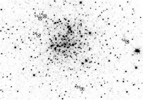
Figure 1: Finding chart for the 5 stars observed in NGC 6528 (HST WFPC2 F814W image). Resolution is 0.1”/px.

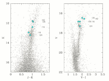
Figure 2: The SOFI near-IR (left) and HST optical (right) CMD of NGC 6528 with the target stars shown as big filled circles.

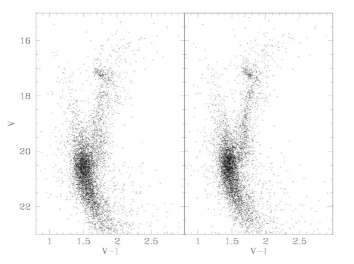
Figure 3: NGC 6528: Original and reddening corrected V vs. V-I Colour Magnitude Diagrams

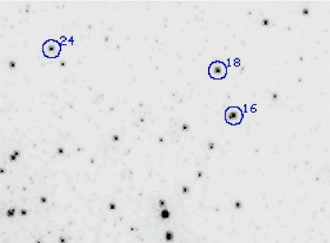
Figure 4: Three program stars I16, I18 and I24 identified in a NIC2 $J$ frame. Resolution is 0.075”/px. The diameter of the circle is 1 arcsec, corresponding to the size of the UVES slit. Star I16 clearly has a nearby companion, not resolved in the ground-based (nor in the WFPC2) images.

A posteriori, we identified some of our targets also in the field of view of a $J,H$ set of NICMOS@HST data (Ortolani et al. 2001). The spatial resolution of the NICMOS observations allowed us to discover that I-16 has in fact a nearby companion which contaminates the spectrum by about 23$\%$ in the J and H bands (see Fig. 4). For this reason, I-16 was discarded from the spectroscopic analysis.

2.2 Spectra

High resolution spectra for five members of NGC 6528, in the wavelength range $\lambda\lambda$ 4800-6800 Å, were obtained with the UVES spectrograph at the ESO VLT. The target membership had been previously verified from radial velocities by Coelho et al. (2001). In what follows we will consider mainly the reddest portion of the spectrum (5800-6800 Å) covered by the MIT backside illuminated and AR coated CCD ESO # 20 of 4096x2048 pixels, of pixel size 15x15$\mu$m. The bluer region was used only to derive the carbon abundance from the C₂ (0,1) bandhead at $\lambda$ 5635 Å. With the UVES standard setup 580, the resolution is R$\sim 45000$ for a 1 arcsec slit width, and R$\sim 55000$ for a slit of 0.8 arcsec. The pixel scale is 0.0174 Å/px. The log of the observations is shown in Table 2.

Table 2: Log of the spectroscopic observations carried out on 2000 June 24-25-26 and 2001 July 6. The quoted seeing is the mean value along the exposures.

Target	V	date/	UT	exp	Seeing	Airmass	(S/N)/px	Slit	${\rm v_{r}^{obs}}$	${\rm v_{r}^{hel.}}$
		Julian day		(s)	(′′)			width	${\rm kms^{-1}}$	${\rm kms^{-1}}$
I-16	17.496	26.06.00	03:46:28	5400	1.0	1.0		1.0′′	208	206
		2451721	05:18:53	5400	0.8	1.0-1.2		”	”	”
I-18	16.732	26.06.00	03:46:28	5400	1.0	1.0	40	1.0′′	211	209
		2451721	05:18:53	5400	0.8	1.0-1.2		”	”	”
I-24	17.194	26.06.00	06:59:18	4584	1.1	1.2-1.6	30	1.0′′	215	213
		2451721	08:37:43	3600	1.3	1.7-2.6		”	”	”
I-36	16.392	26.06.00	00:13:03	5400	1.1	1.2-1.8	40	1.0′′	218	217
		2451721	01:48:35	5400	1.1	1.2-1.0		”	”	”
I-42	16.426	06.07.01	05:29:42	3600	0.7	1.0-1.1	30	0.8′′	222	215
		2452096	06:30:35	3600	0.8	1.2-1.5		”	”	”

The spectra were reduced using the UVES context of the MIDAS reduction package, including bias and inter-order background subtraction, flatfield correction, extraction and wavelength calibration (Ballester et al. 2000). When possible we used the optimal extraction routine, rejecting the cosmic rays. However, in a few cases (e.g. star I16 and I18, which were observed through the same slit), the optimal extraction could not be used, and therefore we turned to the standard extraction routine. The two spectra obtained for each target star were summed before the analysis.

A mean v_r = 215$\pm$5 km s^-1 or heliocentric v${}^{\rm hel}_{\rm r}$ = 212 km s^-1 was found for NGC 6528, higher than the values of 160 kms ^-1 given in Zinn & West (1984) or 143 km s^-1 given in Zinn (1985), but in very good agreement with more recent values of $203\pm 20$ km s^-1 and 212$\pm$16 km s^-1 measured respectively by Minniti (1995) and Rutledge et al. (1997).

3 Stellar Parameters

3.1 Reddening

A reddening of E($B-V$) = 0.55 was given in Momany et al. (2003), however this was a mean value from determinations relative to NGC 6553 and 47 Tucanae, in different colours (see their Table 3), and those values are somewhat dependent on the metallicity and $\alpha$-element assumptions in isochrone models. They can be used as guidelines, but for temperature determinations we need to investigate further about the value to adopt, since a $\Delta$E(B-V) = 0.07 implies in a $\Delta$T_eff $\approx$ 400 K.

Reddening vs. spectral type:

A very well established result, after the analysis of Schmidt-Kaler (1961), is that the absorption (in the $UBV$ bands) is a function of the the energy distribution of the star within the broadband filters (see also more recent discussions and calculations in Olson 1975, Grebel and Roberts 1995, and Fitzpatrick 1999). Such effect is due to the decrease of the extinction, toward longer wavelengths, across the width of the filter. The net effect results in a shift of the effective wavelength, for a reddened star, to a longer wavelength than for an unreddened star. The magnitude of the shift depends on the energy distribution (therefore on the spectral type) of the star. This makes redder (cooler) stars systematically less absorbed. The effect is more pronounced in the B band than in V, for the same amount of interstellar dust, and thus the colour excess becomes sensitive to the stellar energy distribution. Schmidt-Kaler (1961) introduced a parameter $\eta$ to quantify this effect:

$\eta$ = E(B-V)_(SpT)/E(B-V)_B0

and showed that its variation is of the order of 10% from early type stars to M stars. $\eta$ is also slightly dependent on the reddening itself.

NGC 6522 is another globular cluster located in the Baade’s Window that can be used to derive colour excess in the region. The work by Terndrup & Walker (1994) on several fields in NGC 6522 gives E(B-V)=0.52 for B-V=0 stars, corresponding to about 0.44-0.45 for our K-M stars. This is done via a simple fit to CMDs relative to other globular clusters having the same RGB morphology. Terndrup et al. (1998) derived Av=1.4 on a proper motion cleaned CMD of NGC 6522. This gives again about E(B-V)=0.45 for K-M stars. We can conclude that there is quite strong evidence that NGC 6522 has a reddening close to 0.44-0.45. Now we should estimate the difference between NGC 6528 and NGC 6522. A check on Stanek’s (1996) maps indicates that the two regions have very similar extinctions. The zero point has been revised by Alcock et al. (1998) and Gould et al. (1998). Following Alcock et al., from their Table 1, the extinction near NGC 6528 (at $\alpha$=18^h04^m29.46^s, $\delta$=-30^∘01’ 07”, J2000.0) is $\Delta$A_V=0.05 mag higher than near NGC 6522. Using a total-to-selective absorption R = A_V/E(B-V) = 3.1, this transforms into E(B-V)= 0.01 - 0.02 mag, which makes a very small difference. The same authors derived E(B-V)=0.48 for (B-V)=0.0 stars for the less redenned side of the Baade Window, corresponding to one of the lowest values (about 0.42 for K-M stars). They strongly argue against high values. Since they start from luminosity measurements of the RR Lyrae stars, they have to make assumptions about the total-to-selective absorption R_V = A_V/E(B-V) value to get the E(B-V), but still this appears to be a quite firm result.

We carried out an independent reddening measurement for NGC 6522 using HST photometry from Piotto et al. (2002). The CMD of NGC 6522 was compared to those of reference clusters, having comparable metallicities, and which have been observed in with the same HST instrumentation. The reddening difference between NGC 6522 and each reference cluster is measured as the colour difference of their red giant branches, $\Delta$(B-V)_RGB=$\Delta$ E(B-V), as shown in Table 3.

A cluster metallicity can be estimated from the curvature of the RGB, since more metal-rich giants show progressively fainter RGB magnitudes (as well as redder RGB colours), due to higher blanketing (Ortolani et al. 1990, 1991). The metallicities reported are from Harris (1996, as updated in http://physun.physics.mcmaster.ca/Globular.html). Note that the more metal rich clusters will give obviously a bit lower reddening and viceversa: M 13, NGC 6681 and NGC 1904 appear to have a more metal poor morphology as concerning the RGB, and give higher $\Delta$(B-V). The E(B-V) = $\Delta$(B-V) would be given by comparing two clusters of same metallicity, given that there should be no blanketing differences between them. The best morphological fits are obtained for NGC 5904 (M5), NGC 1851 and NGC 6266. Harris (1996) gives [Fe/H]=-1.44 for NGC 6522, and in these cases the derived $\Delta$(B-V) is close to the E(B-V) value. In conclusion, it seems that E(B-V)=0.42-0.50 represents a fiducial reddening value for NGC 6522 for the colour of horizontal branch to G-K stars.

In order to obtain the reddening for NGC 6528 we would have to add the reddening difference between the former and NGC 6522 (+0.02), but another $\Delta$E(B-V)$=-0.02$ would be needed to translate this for K-M stars (c.f. parameter $\eta$ defined above). Therefore, for our stars, we adopt the same reddening E(B-V)=$0.46\pm 0.04$ determined above for NGC 6522. Note that this result is independent of possible zero point errors in the Piotto et al. photometry because it is based on differential photometry.

Yet another free parameter comes into play, because the extinction law towards the bulge is somewhat controversial. Extremely low values of the total-to-selective absorption R_V = A_V/E(B-V) were recently proposed by e.g. Udalski (2003) in the galactic bulge OGLE II field, as opposed to the traditional R_V=3.1 from Cardelli et al. (1989) or Rieke & Lebofsky (1985). For completeness, let us recall that the total-to-selective absorption R_V depends on the amount of reddening (Olson 1975) and on metallicity (Grebel & Roberts 1995), as discussed in Barbuy et al. (1998), and the value should be somewhat higher for high reddening and high metallicity values. If lower R_V values are assumed, our resulting dereddened colours will be redder, and therefore the deduced effective temperatures will be cooler.

For the present analysis we adopt E(B-V) = 0.46 for NGC 6528 and the extinction law given by Dean et al. (1978) and Rieke & Lebofsky (1985), namely: R_V = 3.1, E($V-I$)/E($B-V$)=1.33, E($V-K$)/E($B-V$)=2.744 and E($J-K$)/E($B-V$)=0.527 (Table 1).

Table 3: Reference clusters, respective metallicities (according to Harris (1996)), and $\Delta$(B-V) corresponding to the reddening of NGC 6522 derived differentially relative to the comparison clusters.

comparison cluster	[Fe/H]	$\Delta$(B-V)
M 13	-1.54	0.60
NGC 6229	-1.43	0.50
NGC 6723	-1.12	0.50
NGC 6681	-1.51	0.60
NGC 6266	-1.29	0.42
NGC 5904	-1.27	0.50
NGC 1851	-1.22	0.47
NGC 1904	-1.57	0.55

Table 4: Stellar parameters derived using the calibrations by Alonso et al. (1999; AAM99) for $V-I$, $V-K$, $J-K$. The dereddened colours were obtained using the reddening law by Dean et al. (1978) and Rieke & Lebofsky (1985).

	AAM99
star	Teff(V-I)	Teff(V-K)	Teff(J-K)	Teff (mean)	${\rm BC_{V}}$	${\rm M_{bol}}$	log g
I-18	4504	4520	4409	4511	–0.47	–0.16	2.0
I-36	4071	4051	3937	4019	–0.87	–0.93	1.5
I-42	3897	3975	3937	3936	–0.97	–0.93	1.5

3.2 Temperatures

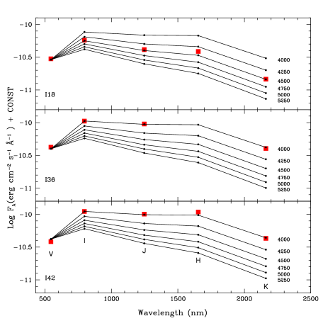
Figure 5: Calibrations of Alonso et al. (1999), of $V$, $I$, $J$, $H$ and $K$ as a function of effective temperature (solid lines), where the magnitudes for the sample stars are overplotted (filled squares).

Effective temperatures were derived from $V-K$, $V-I$ and $J-K$ using the colour-temperature calibrations by Alonso et al. (1999) together with the reddening laws by Dean et al. (1978) and Rieke & Lebofsky (1985). The T_eff derived from each colour are listed in Table 4. We have excluded from the spectroscopic analysis the star I-16 as explained in Sect. 2.1, and also star I-24, being a suspect unresolved binary, for the reasons explained below (Sect. 4). In order to verify that all the colours are compatible with the adopted temperature, we compared the spectral energy distribution (SED) of our targets with the prediction by Alonso et al. (1999). Fig. 5 shows the flux obtained from the $V,I,J,H$ and $K$ magnitudes, together with Alonso et al.’s calibrations for stars of different temperatures (4000-5250 K). Since Alonso et al. give a relation between colours and temperatures, the predicted flux in each band was obtained by assuming an arbitrary value for the $V$ magnitude. A vertical shift was then allowed to match the SEDs of the sample stars.

3.3 Gravities

The classical relation $\log g_{*}=4.44+4\log(T_{*}/T_{\odot})+0.4(M_{\rm bol}-4.75)+\log(M_{*}/M_{\odot}$) was used, adopting T_⊙ = 5770 K, M_∗ = 0.85 M_⊙ and M_bol⊙ = 4.75 (Cram 1999).

A distance modulus of (m-M)₀ = 15.10 was adopted from Harris (1996) together with a reddening of E($B-V$) = 0.46 and A_V = 1.43, as discussed in the previous sections. The bolometric corrections from Alonso et al. (1999) and corresponding gravities are given in Table 4.

Spectroscopic gravities were also derived by imposing ionization equilibrium between FeI and FeII lines (see Sect. 4).

4 Equivalent widths and oscillator strengths

The equivalent widths have been measured using a new automatic code developed by P. Stetson (DAOSPEC, Stetson et al. 2004, in preparation). This routine fits a Gaussian profile to all lines, imposing a constant FWHM. In order to take into account the broader profile of strong lines, we manually measured lines stronger than 140 mÅ allowing a best fit for the FWHM of each line. Star I-24 shows lines with FWHM significantly larger than that of the other stars (a factor of 1.5), and most of the lines have a systematic asymmetry (Fig. 6). This was interpreted as evidence of the presence of an unresolved companion, and for this reason the star was excluded from the following analysis. Note that at lower spectral resolution such unresolved binaries would not have been detected, and therefore the results would not have reflected the true stellar abundances.

Figure 6: Spectrum of I24 showing its probable binary nature.

The Fe I line list and respective oscillator strengths given in NIST (Martin et al. 2002) and some lines with gf-values from McWilliam & Rich (1994, hereafter MR94) were used to derive spectroscopic parameters. Eight measurable Fe II lines, and their respective oscillator strengths from Biémont et al. (1991), and renormalized by Meléndez & Barbuy (2004, in prepararion), were used to obtain ionization equilibrium.

The damping constants were computed where possible, and in particular for most of the Fe I lines, using the collisional broadening theory of Barklem et al. (1998, 2000 and references therein). For lines of Si, Ca and Ti the derived values of the interaction constant C₆, where C₆ = 6.46E-34 ($\sigma$/63.65)^5/2, $\sigma$ being the cross section of collision computed by Barklem et al., which is related to the collisional damping constant $\gamma_{6}$ = 17v^3/5C${}_{6}^{2/5}$N, are reported in Table 6. Otherwise a fit to the solar spectrum or standard van der Waals values (Unsöld 1955; Gray 1976) are employed.

The oscillator strengths of Na, Mg, Si, Ca and Ti lines given by Brown & Wallerstein (1992), MR94, the NIST database (Martin et al. 2002), Barbuy et al. (1999) from fits to the solar spectrum, the VALD database (Kupka et al. 1999), and the recent compilation by Bensby et al. (2003) are reported in Table 6. The adopted oscillator strengths for these lines were then selected from a fit to the solar spectrum observed with the same VLT-UVES instrumentation, adopting a NMARCS solar atmospheric model (Edvardsson et al. 1993), in order to be compatible with the model grid used to analyse the sample giants. These gf-values were checked against the spectrum of Arcturus (Hinkle et al. 2000), by adopting the stellar parameters derived by Meléndez et al. (2003), namely T_eff = 4275 K, log g = 1.55, [Fe/H] = -0.54, v_t = 1.65 km s^-1 and abundances [C/Fe] = -0.08, [N/Fe] = +0.3, [O/Fe] = +0.43, and other abundance ratios from the literature, and rederived from our fits: [Na/Fe] = +0.1, [Mg/Fe] = +0.35, [Al/Fe] = +0.3, [Si/Fe] = +0.25, [Ca/Fe] = +0.1, [Ti/Fe] = +0.3. The selected gf-values are marked in bold face in Table 6.

For the oxygen forbidden line [OI]6300 Å we adopt the oscillator strength recently derived by Allende Prieto et al. (2001): log gf = -9.716.

For lines of the heavy elements BaII, LaII and EuII, a hyperfine structure was taken into account, based on the hyperfine constants by Lawler et al. (2001a) for EuII, Lawler et al. (2001b) for LaII and Biehl (1976) for BaII.

Solar abundances were adopted from Grevesse et al. (1996), except for the value for oxygen where $\epsilon$(O) = 8.77 was assumed, as recommended by Allende Prieto et al. (2001) for the use of 1-D model atmospheres.

5 Iron abundances

Photospheric 1-D models for the sample giants were extracted from the NMARCS grid (Plez et al. 1992), originally developed by Bell et al. (1976) and Gustafsson et al. (1975).

The LTE abundance analysis and the spectrum synthesis calculations were performed using the codes by Spite (1967, and subsequent improvements made in the last thirty years), Cayrel et al. (1991) and Barbuy et al. (2003).

The stellar parameters were derived by initially adopting the photometric effective temperature and gravity, and then further constraining the temperature by imposing excitation equilibrium for Fe I lines and the gravity by imposing ionization equilibrium for Fe I and Fe II. Microturbulence velocity v_t was determined by canceling the trend of Fe abundance vs. equivalent width.

The same method and the same line list, applied to the Sun and Arcturus, yield metallicities of [Fe I/H] = 0.09, [Fe II/H] = 0.01 and [Fe I/H] = -0.49, [Fe II/H] = -0.56 respectively. Note that in this case the stellar parameters that we converged to are T_eff 5800 K, log g = 4.4, v_t = 1.0 km s^-1 for the Sun and T_eff = 4300 K, log g = 1.8, v_t = 1.6 km s^-1 for Arcturus, in good agreement with expectations.

Table 5 reports [Fe I/H] and [Fe II/H] values for the sample stars. Figs. 7, 8 and 9 illustrate the results of the analysis for stars I-18, I-36 and I-42 respectively. The abundances from Fe II lines for star I-42 showed relatively large scatter, possibly due to a combination of the lower S/N and cooler temperature. We therefore compared the equivalent width of Fe II lines in I-42 with those of I-36, having very similar T_eff, and rejected the lines showing large deviations from the mean percent difference. This allowed us to have a smaller dispersion in [Fe II/H] and therefore to get a spectroscopic constraint on the gravity for I-42.

A second set of parameters based on the photometry was derived by imposing the temperature and gravity values from Table 4 and determining the metallicity and the microturbulence velocity from Fe I and Fe II. The two sets of stellar parameters are given in Table 5.

As a check ionization equilibrium was also used as a temperature indicator, as suggested by McWilliam & Rich (2003, hereafter MR03), keeping the gravity fixed to its photometric value, and varying the temperature to recover the Fe ionization equilibrium. This leads to temperatures in better agreement with the photometric values, while keeping excitation equilibrium virtually identical to the formally best fitting spectroscopic temperature.

This shows that the true temperature of the sample stars is very likely hotter (by $\sim 200$ K) than the photometric one. In the following we will keep this last set of parameters as the one which gives the most self consistent picture. The errors on [Fe/H] were estimated as follows. The formal error on the slope in the FeI $vs.$ ionization potential implies an error in the temperature of $\pm$100 K for all the stars. From the abundance analysis of Arcturus, we estimated that a variation of $\pm$ 100 K in the temperature propagates into a difference of $\pm$0.07 in [FeI/H] and $\pm 0.06$ in [FeII/H]. This variation in the metallicity of Arcturus was found by forcing excitation equilibrium (i.e, by fixing the gravity) and canceling the trend in abundance with E.W. (i.e., by fixing $v_{t}$) with the new (uncertain by $\pm 100$ K) temperatures. This procedure gives an estimate of the systematic error due to a possible uncertain assumption on the input parameters. The statistical error, measured from the spread in abundance obtained from different lines, is 0.018 $<$ $\Delta$[FeI/H] $<$ 0.026 for the three stars. The final error, being the quadratic sum of the systematic and statistical components, is quoted in Table 5.

Table 5: Stellar parameters and derived metallicities

star	${\rm T_{eff}}$	${\rm log\;g}$	${\rm[FeI/H]}$	${\rm[FeII/H]}$	${\rm v_{t}(km/s)}$
Spectroscopic:
I-18	4800	2.3	+0.05 ($\pm 0.072$)	–0.07 ($\pm 0.08$)	1.5
I-36	4300	1.8	–0.04 ($\pm 0.073$)	–0.08 ($\pm 0.10$)	1.5
I-42	4200	1.6	–0.16 ($\pm 0.075$)	–	1.3
Photometric:
I-18	4500	2.0	–0.05 ($\pm 0.072$)	+0.18 ($\pm 0.08$)	1.3
I-36	4000	1.5	+0.00 ($\pm 0.073$)	+0.35 ($\pm 0.10$)	1.5
I-42	4000	1.5	–0.19 ($\pm 0.075$)	–	1.3
Ionization temperature:
I-18	4700	2.0	–0.05 ($\pm 0.072$)	–0.11 ($\pm 0.08$)	1.5
I-36	4200	1.5	–0.13 ($\pm 0.073$)	–0.09 ($\pm 0.10$)	1.5
I-42	4100	1.6	–0.14 ($\pm 0.073$)	–0.08 ($\pm 0.10$)	1.2

Figure 7: Iron abundance for each line measured in I-18. Abundances of FeI and FeII are shown as a function of both $\chi_{ex}$ and E.W. in the different panels. The lines shown with a cross have been excluded from the computation of the mean abundance, using a $\sigma$ clipping criterion. The flattening of the FeI abundance with $\chi_{ex}$ and E.W. has been used to set constraints on the temperature and microturbulence velocity, respectively.

Figure 8: Same as Fig. 7 for star I-36.

Figure 9: Same as Fig. 7 for star I-42.

6 Abundance ratios

Elemental abundances were obtained through line-by-line spectrum synthesis calculations, for the line list given in Tables 6 and 7.

The calculations of synthetic spectra were carried out as described in Cayrel et al. (1991) and Barbuy et al. (2003), where molecular lines of CN (A²$\Pi$-X²$\Sigma$), C₂ Swan (A³$\Pi$-X³$\Pi$), TiO (A³$\Phi$-X³$\Delta$) $\gamma$ and TiO (B³$\Pi$-X³$\Delta$) $\gamma$’ systems are taken into account. As a first guess, the abundances obtained from the equivalent width, in the “classical” way, without taking into account the effect of molecules, were adopted. These first guess values are listed in Table 8.

The comparison between the synthetic spectrum, generated including the effects of molecules, and the observed one, for each line in Table 6, allowed us to set a more realistic estimate of the true abundance ratios. Our best values are listed in Table 9. The comparison between Table 8 and Table 9 gives an estimate of the importance of the effect of molecule formation in the atmosphere of each star. The main effect is a lowering of the continuum as illustrated in Fig 10, where TiO was computed for [O/Fe]=[Ti/Fe]$=0.0$ and +0.2 (the latter value is the adopted one), and for T${}_{\rm eff}=4000$, 4100 and 4200 K.

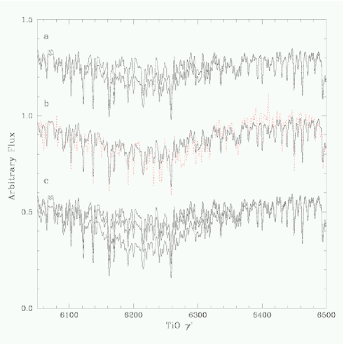
Figure 10: TiO $\gamma$’ bandhead in star I-42, where spectra are convolved with gaussians of FWHM = 2.0 Å: a) computed with [O/Fe]=[Ti/Fe] = 0.0 and +0.2 (adopted value); b) comparison of the observed spectrum (dotted line) with model computed with T_eff = 4100 K and [O/Fe]=[Ti/Fe]=+0.2; c) T_eff = 4000, 4100 and 4200 K.

Errors in the abundance ratios can be due essentially to gf-values and damping constants used. They can be deduced from Table 6, where a difference of 0.2 dex in log gf essentially means a difference of 0.2 dex in abundance, for a given damping constant.

The carbon abundance [C/Fe] = 0.0 was derived for the 3 sample stars, based on the C₂(0,1) 5635 Å, whereas the nitrogen abundance [N/Fe] = +0.6 was derived from a series of CN bandheads along the spectrum. The region of the C₂ line is very noisy, and the whole region is blended with CN lines as well, such that the carbon abundance is not as precise as all the other derivations in this work. On the other hand, C+N is reliable. The N overabundance corresponds to a mixing that is expected in giants, bringing carbon down and nitrogen up, but since C+N is high, it does possibly involve as well a primordial enhancement in C+N elements, as detected before in NGC 6553 (Meléndez et al. 2003).

Figs. 11, 12, 13 show examples of the fit of Oxygen, Calcium and Titanium lines, respectively, in the three sample stars. While the abundance of [O/Fe] and [Ca/Fe] is very homogeneuos in the three stars, Titanium is considerably higher in star I-42. Fig. 13 shows, for comparison, also a model with low Ti ([Ti/Fe]=-0.2) with the stellar parameters of I-42. Clearly such low Ti for I-42 can be excluded from the present data.

The fit of the Oxygen line [OI]6300.311 Å shown in Fig. 11 also shows the nearby ScII 6300.67 line. Sneden & Primas (2001) pointed out that the ratio of [OI] to ScII lines is a more reliable measure of the oxygen enhancement. Indeed, OI and ScII are the dominant species of these elements in cool stellar atmospheres, and excitation potentials of the [OI]6300.31 Å ($\chi_{ex}$ = 0.0 eV ) and that of ScII6300.67 Å ($\chi_{ex}$ = 1.5 eV) are similar. We used a hyperfine structure splitting and corresponding log gf of the ScII line as given in Spite et al. (1989). The present analysis gives [O/Sc]=+0.35, +0.35 and +0.20 for I-18, I-36 and I-42, respectively.

The line-by-line abundance ratios are given in Table 6, while the final resulting abundance ratios for the 3 sample stars, together with their mean, are shown in Table 9. Column 7 lists the results for the 4 HB stars analysed by C01 and column 8 shows the average of Baade’s Window 11 K giants analysed by MR94. There is a general good agreement with respect to C01, except for a difference of 0.2 dex in [FeI/H], and the Si, Ca and BaII abundances which are higher in their study. The Mg, Al and Ti abundances found by MR94 in Baade’s Window are higher than the values found in the present paper and in C01.

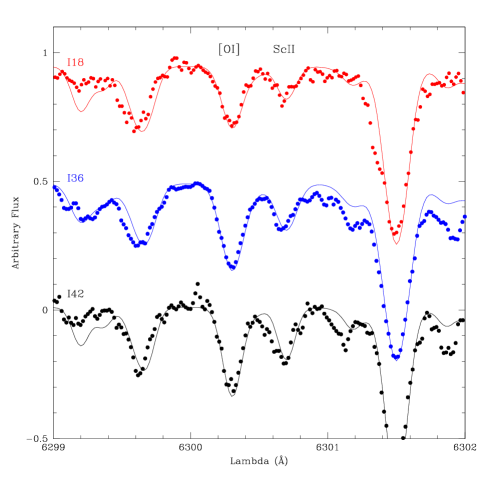
Figure 11: Fit of the [OI]6300.311 Å line in the program stars.

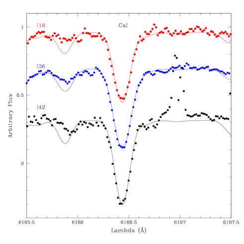
Figure 12: Fit of the CaI 6166.44 Å line in the program stars.

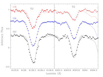
Figure 13: Fit of the TiI 6126.224 and 6303.77 Å lines in the program stars.

Table 6: Abundance ratios using the “Ionization temperature” set of parameters given in Table5. (^a): C₆ computed using collisional broadening theory by Barklem et al. (1998, 2000).

Species	$\lambda$	$\chi_{ex}$	C6	loggf						[X/Fe]
				$---------------------$						$----------$
	(${\rm\AA}$)	(eV)		BW92	MR94	NIST	B99	VALD	BFL03	$\alpha$Boo	I-18	I-36	I-42
NaI	6154.230	2.10	0.90E-31	-1.53	-1.57	-1.56	-1.56	-1.56	-1.57	0.00	+0.65	+0.40	+0.30
NaI	6160.753	2.10	0.30E-31	-1.23	-1.27	-1.26	-1.26	-1.26	-1.27	+0.10	+0.60	+0.40	+0.30
MgI	6318.720	5.11	0.30E-30	–	–	–	-2.10	-1.72	–	+0.35	+0.00	-0.05	+0.05
MgI	6319.242	5.11	0.30E-31	–	-2.22	–	-2.36	-1.95	–	+0.35	+0.15	-0.05	+0.05
MgI	6319.490	5.11	0.30E-31	–	–	–	-2.80	-2.43	–	+0.35	+0.00	-0.05	+0.05
MgI	6765.450	5.75	0.30E-31	–	-1.94	–	-1.94	–..	–	–	+0.00	+0.05	+0.25
SiI	5948.548	5.08	2.19E-30a	-1.23	–	-1.24	-1.17	-1.23	-1.13	+0.35	+0.10	+0.10	+0.05
SiI	6142.494	5.62	0.30E-31	-1.39	–	–	-1.50	-0.92	-1.50	+0.30	+0.05	+0.10	–
SiI	6145.020	5.61	0.30E-31	-1.32	–	–	-1.45	-0.82	-1.46	+0.25	+0.05	+0.10	+0.05
SiI	6155.142	5.62	0.30E-30	-0.55	–	–	-0.85	-0.40	-0.72	+0.30	+0.10	+0.10	+0.15
SiI	6237.328	5.61	0.30E-30	-0.84	-1.01	–	-1.15	-0.53	-1.05	+0.20	+0.05	+0.10	–
SiI	6243.823	5.61	0.30E-31	-1.15	–	–	-2.32	-0.77	-1.30	+0.30	+0.05	+0.10	+0.05
SiI	6414.987	5.87	0.30E-30	-0.89	–	–	-1.13	-1.10	–	+0.35	+0.20	+0.20	–
SiI	6721.844	5.86	0.90E-30	-0.94	-1.17	-0.94	-0.94	-1.49	–	+0.10	+0.00	+0.10	+0.10
CaI	6102.727	2.52	4.54E-31a	-0.79	–	-0.79	-0.24	-0.96	–	+0.10	-0.30	-0.40	-0.40
CaI	6156.030	2.52	0.30E-31	–	–	-2.20	-2.39	-2.50	–	+0.10	-0.35	-0.30	-0.40
CaI	6161.295	2.51	5.98E-31a	-1.03	–	-1.02	-1.25	-1.29	-1.26	+0.10	-0.35	-0.40	-0.40
CaI	6162.167	2.52	5.95E-31a	-0.80	–	-0.09	-0.10	-0.17	–	+0.10	-0.30	–	–
CaI	6166.440	2.52	5.95E-31a	-1.14	-1.14	-0.90	-1.07	-1.16	-1.17	+0.10	-0.30	-0.40	-0.30
CaI	6169.044	2.52	5.95E-31a	-0.80	-0.80	-0.54	-0.71	-0.81	-0.84	+0.10	-0.20	-0.40	-0.40
CaI	6169.564	2.52	5.95E-31a	-0.48	-0.48	-0.27	-0.27	-0.93	-0.63	+0.10	-0.40	-0.40	–
CaI	6439.080	2.52	5.12E-32a	+0.47	–	+0.47	-0.04	+0.39	+0.3	+0.10	-0.30	-0.40	-0.40
CaI	6455.605	2.52	5.06E-31a	–	–	-1.35	-1.35	-1.56	-1.30	+0.15	-0.40	-0.40	-0.40
CaI	6464.679	2.52	5.09E-32a	–	–	–	-2.10	-4.27	–	+0.10	–	0.00	-0.60
CaI	6471.668	2.52	5.09E-32a	-0.69	–	-0.59	-1.00	-0.65	-0.65	+0.10	-0.30	-0.30	–
CaI	6493.788	2.52	5.05E-32a	-0.11	–	+0.14	+0.60	+0.02	-0.19	+0.10	-0.35	-0.30	-0.40
CaI	6499.654	2.52	5.05E-32a	-0.82	–	-0.59	-0.63	-0.72	-0.73	+0.10	-0.30	-0.30	-0.40
CaI	6508.846	2.52	0.30E-31	-2.41	-2.50	-2.11	-2.51	-2.16	–	+0.15	-0.20	-0.40	-0.20
CaI	6572.779	0.00	2.62E-32a	-4.31	-4.31	-4.29	-4.30	-4.10	–	+0.10	-0.40	-0.60	-0.20
CaI	6717.687	2.71	0.70E-30	–	–	-0.61	-0.61	-0.60	–	+0.20	-0.30	-0.40	-0.40
CaI	6719.687	2.71	0.70E-30	-2.41	-2.55	–	-2.80	–	–	+0.10	–	–	–
TiI	5866.452	1.07	2.16E-32a	-0.84	–	-0.84	-0.75	-0.84	–	-0.40	-0.20	-0.20	+0.10
TiI	5922.110	1.05	3.46E-32a	-1.47	–	-1.47	-1.47	-1.47	–	-0.40	-0.30	-0.20	+0.20
TiI	5965.835	1.88	2.14E-32a	-0.41	–	-0.41	-0.50	-0.41	–	-0.40	-0.30	-0.30	+0.10
TiI	5978.549	1.87	2.14E-32a	-0.50	–	-0.50	-0.51	-0.50	–	-0.30	-0.40	-0.20	+0.10
TiI	6064.626	1.05	2.06E-32a	-1.94	–	-1.94	-2.78	-1.94	–	-0.40	-0.30	-0.20	+0.20
TiI	6091.177	2.27	3.89E-32a	-0.42	–	-0.42	-0.32	-0.42	–	-0.30	-0.30	-0.20	+0.10
TiI	6126.224	1.07	2.06E-32a	-1.42	–	-1.43	-1.30	-1.43	-1.37	-0.30	-0.30	-0.20	+0.20
TiI	6258.110	1.44	4.75E-32a	-0.35	–	-0.36	-0.51	-0.36	–	-0.40	-0.30	-0.30	+0.10
TiI	6261.106	1.43	4.68E-32a	-0.48	–	-0.48	-0.66	-0.48	-0.42	-0.50	-0.35	-0.30	+0.20
TiI	6303.767	1.44	1.53E-32a	–	-1.57	-1.57	-1.57	-1.57	-1.51	-0.30	-0.30	-0.20	+0.20
TiI	6336.113	1.44	0.30E-31	–	-1.74	-1.74	-1.79	-1.74	–	-0.30	-0.20	-0.20	+0.20
TiI	6508.154	1.43	1.46E-32a	–	-2.05	–	-2.20	-2.15	–	–	-0.30	-0.20	+0.20
TiI	6554.238	1.44	2.72E-32a	-1.22	-1.22	-1.22	-1.22	-1.22	–	-0.30	-0.20	-0.20	+0.20
TiI	6556.077	1.46	2.74E-32a	-1.07	-1.07	-1.07	-1.07	-1.07	–	-0.35	-0.05	-0.30	+0.20
TiI	6599.113	0.90	2.94E-32a	-2.09	–	-2.09	-3.00	-2.09	–	-0.35	-0.30	-0.20	+0.10
TiI	6743.127	0.90	0.30E-31	–	-1.63	-1.63	-1.68	-1.63	-1.63	-0.40	-0.35	-0.30	+0.10
TiII	6491.580	2.06	0.30E-31	–	–	-2.10	-2.10	-1.79	–	-0.30	-0.30	-0.20	+0.10
TiII	6559.576	2.05	0.30E-31	–	-2.48	–	-2.60	-2.02	–	–	-0.10	-0.30	–
TiII	6606.970	2.06	0.30E-31	–	–	-2.79	-3.00	-2.79	-2.76	-0.30	-0.20	-0.20	+0.00

Table 7: C, N, O and heavy elements. Carbon abundances are derived from C₂ lines and nitrogen abundances from CN lines (Sect. 6). Abundances of the heavy elements Ba, La and Eu are derived using hyperfine structure (Sect. 4).

Species	$\lambda({\rm\AA})$	$\chi_{ex}$(eV)	log gf	I-18	I-36	I-42
[OI]	6300.311	0.00	–9.716	+0.10	+0.15	+0.20
ScII	6300.67	1.50	hfs	-0.25	-0.20	+0.00
C(C2)	5634.2,35.5	(0,1)	–	0.00	0.00	0.00
N(CN)	6332.2	(5,1)	–	+0.60	+0.60	+0.60
BaII	6141.727	0.70	hfs	-0.20	-0.15	+0.10
BaII	6496.908	0.60	hfs	-0.15	-0.15	+0.10
LaII	6390.480	0.32	hfs	0.00	-0.15	+0.20
EuII	6645.127	1.38	hfs	0.00	+0.10	+0.10

Table 8: First guess abundance ratios [X/Fe] of the program stars

Species	No.	I-18	I-36	I-42
[AlI/Fe]	2	-0.15	+0.00	+0.15
[NaI/Fe]	2	+0.62	+0.30	+0.18
[MgI/Fe]	4	+0.24	+0.15	+0.31
[SiI/Fe]	3	+0.12	+0.08	+0.11
[CaI/Fe]	7	–0.30	–0.41	–0.28
[TiI/Fe]	6	–0.30	–0.08	+0.23
[TiII/Fe]	1	–0.15	–	+0.26

Table 9: Final abundance ratios [X/Fe] of the program stars

Species	No.	I-18	I-36	I-42	mean	C01	MR94
[FeI/H]	50	–0.05	–0.13	–0.14	–0.11	+0.07	–
[OI/Fe]	1	+0.10	+0.15	+0.20	+0.15	+0.07	+0.03
[OI/Sc]	1	+0.35	+0.35	+0.20	+0.30	+0.17	–
[NaI/Fe]	2	+0.60	+0.40	+0.30	+0.43	+0.40	+0.20
[MgI/Fe]	4	+0.05	+0.05	+0.10	+0.07	+0.14	+0.35
[SiI/Fe]	3	+0.05	+0.10	+0.10	+0.08	+0.36	+0.14
[CaI/Fe]	7	–0.40	–0.40	–0.40	–0.40	+0.23	+0.14
[TiI/Fe]	6	–0.30	–0.20	+0.20	–0.10?	+0.03	+0.37
[TiII/Fe]	1	–0.20	–0.20	+0.05	–0.12?	–	–

7 Discussion and Conclusions

We have derived element abundances for three giants in the globular cluster NGC 6528. Five targets were originally selected. However, the high spatial resolution of the HST/NICMOS imaging frames, and the high UVES spectral resolution showed that two of them are in fact a blend of two stars (I-24 is likely a physical binary), and for this reason the two objects have been excluded from the analysis.

This case shows how strong can be the effect of projection or physical binaries in similar studies, when high spatial resolution images of the field are not available.

From the abundance analysis we conclude that Iron is about solar: [Fe/H]$\sim-0.1$.

The odd-Z element sodium, built up during carbon burning, is strongly overabundant ([Na/Fe]$\sim$ 0.4).

The $\alpha$-elements show a quite peculiar behaviour. O, Mg and Si are just slightly above the solar value ([O/Fe] $\sim$[Mg/Fe]$\sim$ [Si/Fe]$\sim$0.1) while Ca and Ti are underabundant with respect to the Sun ([Ca/Fe]$\sim-0.40$ [Ti/Fe]$\sim-0.2$). It is also somehow puzzling that despite the very good agreement between the abundances derived from different lines in the same star (Table 6), the three stars show a spread in [Ti/Fe]. In particular, star I-42 shows a higher Ti abundance with respect to the other two. Given its radial velocity, the similarity with I-18 and I-36 in the abundances of all the other elements, and the agreement between its photometric and spectroscopic temperature, we tend to discard the hypothesis of it being a field star just accidentally projected on the cluster RGB sequence. We rather believe that its low temperature makes stronger the effect of the TiO molecules in its atmosphere, which also increases our uncertainty in the abundance analysis.

The comparison between our values and the ones in Carretta et al. (2001) reveals some discrepancies in Si, Ca, and Ti. While the different treatment of molecules in the two analyses (Carretta et al. did not account for them) might explain part of the discrepancy, the large (0.6 dex) difference in the Ca abundance has to arise from some other factor. From an independent analysis of the equivalenth widths of the NGC6528 stars observed by Carretta et al. (2001), MR03 found [Ca/Fe]=+0.2, much closer to the value found here. Comparing the three analyses, it seems that the most probable source of discrepancy is the adopted broadening factors. Indeed, it must be noted that all the CaI lines are rather strong, in the saturation regime of the curve of growth.

In fact the abundances of Ca and Ti do not always follow the other $\alpha$-elements, as is the case for example with 47 Tucanae where Ca-to-Fe is solar, and the other $\alpha$s are overabundant (Brown & Wallerstein 1992; Alves-Brito et al. 2004). According to Woosley (private communication), there is metallicity sensitivity in the yields because the mass loss varies with metallicity. The yields therefore strongly depend on the mass loss, such that Ca and Ti show variable proportions in different sites (Woosley & Weaver 1995), and [Ti/Si] is often low.

From our analysis we find a modest enhancement of O, Mg and Si, which is consistent with the trend of a lower $\alpha$-enhancement for the metal-rich end of the bulge field stars found by McWilliam & Rich (2003). However, the predictions by Matteucci & Brocato (1990) and Matteucci, Romano and Molaro (1999) give higher expected values for O and Mg ([O/Fe] $\sim$ [Mg/Fe] $\sim$ +0.6 at [Fe/H] = 0.0, and somewhat less for Si and Ca ([Si/Fe] $\sim$ [Ca/Fe] $\sim$ +0.3). On the other hand, the low values of [Ca/Fe] $\approx$ [Ti/Fe] $\approx$ [Eu/Fe] $\approx$ 0.0 might indicate that there has been a deficiency of SNII of low mass, as pointed out in MR03, and according to predictions by Woosley & Weaver (1995). It is also worth noticing that Ca underabundance is very common in elliptical galaxies (e.g. Thomas et al. 2003 for a discussion of possible causes).

The s-process elements Ba, La tend to show underabundances which is expected for an old population. The s-processing takes place in massive stars (Raiteri et al. 1993), as well as in relatively short lived and long lived intermediate mass stars (Gallino et al. 1998), indicating that there has been no significant contribution from long lived stars.

- (1) Alcock, C., Allsman, R.A., Alves, D.R. et al. (MACHO Project) 1998, ApJ, 494, 396
- (2) Alonso, A., Arribas, S., Martínez-Roger, C. 1999, A&AS, 140, 261 (AAM99)
- (3) Allende Prieto, C., Lambert, D.L., Asplund, M. 2001, ApJ, 556, L63
- (4) Brito, A., Barbuy, B., Ortolani, S., et al. 2004, A&A, submitted
- (5) Ballester, P., Modigliani, A., Boitquin, O. et al. 2000, The Messenger, 101, 31
- (6) Barbuy, B., Bica, E., Ortolani, S. 1998, A&A, 333, 117
- (7) Barbuy, B., Renzini, A., Ortolani, S., Bica, E., Guarnieri, M.D., 1999, A&A, 341, 539
- (8) Barbuy, B., Perrin, M.-N., Katz, D. et al. 2003, A&A, 404, 661
- (9) Barklem, P.S., Anstee, S.D., O’Mara, B.J. 1998, PASA, 15, 336
- (10) Barklem, P.S., Piskunov, N.E., O’Mara, B. J. 2000, A&AS, 142, 467
- (11) Bell, R.A., Eriksson, K., Gustafsson, B., Nordlund, , 1976, A&AS, 23, 37
- (12) Bensby, T., Feltzing, S., Lundström, I. 2003, A&A, 410, 527
- (13) Biehl, D., 1976, PhD thesis, University of Kiel
- (14) Biémont, E., Baudoux, M., Kurucz, R.L., Ansbacher, W., Pinnington, A.E., 1991, A&A, 240, 539
- (15) Brown, J.A., Wallerstein, G. 1992, AJ, 104, 1818
- (16) Cardelli, J.A., Clayton, G.C., Mathis, J.S., 1989, ApJ, 345, 245
- (17) Carretta, E., Cohen, J.G., Gratton, R.G., Behr, B.B. 2001, AJ, 122, 1469 (C01)
- (18) Cayrel, R., Perrin, M.-N., Barbuy, B., Buser, R., 1991 A&A, 247, 108
- (19) Coelho, P., Barbuy, B., Perrin, M.-N. et al., 2001, A&A, 376, 136
- (20) Cohen, J.G., Gratton, R.G., Behr, B., Carretta, E., 1999, ApJ, 523, 739
- (21) Cram, L. 1999, Trans. IAU XXIIIB, ed. J. Andersen, p. 141
- (22) Dean, J.F., Warpen, P.R., Cousins, A.J.: 1978, MNRAS, 183, 569
- (23) Edvardsson, B., Andersen, J., Gustafsson, B. et al. 1993, A&A, 102, 603
- (24) Feltzing, S., Johnson, R.A. 2002, A&A, 385, 67
- (25) Fitzpatrick E.L., 1999, PASP, 111,63
- (26) Gallino, R., Arlandini, C., Busso, M. et al. 1998, ApJ, 497, 388
- (27) Gould, A., Popowski, P., Terndrup, D.M. 1998, ApJ, 492, 778
- (28) Gray, D.F. 1976, The Observation and Analysis of Stellar Photospheres, John Wiley & Sons, New York
- (29) Grebel, E.K., Roberts, W. 1995, A&AS, 109, 293
- (30) Grevesse, N., Noels, A., & Sauval, J. 1996, in ASP Conf. Ser. 99, Cosmic Abundances, ed. S. S. Holt & G. Sonneborn (San Francisco: ASP), 117
- (31) Gustafsson, B., Bell, R.A., Eriksson, K., Nordlund, , 1975, A&A, 42, 407
- (32) Harris, W.E. 1996, AJ, 112, 1487
- (33) Hinkle, K., Wallace, L., Valenti, J., Harmer, D. 2000, Visible and Near Infrared Atlas of the Arcturus Spectrum 3727 - 9300 , ASP, San Francisco
- (34) Kupka, F.G., Piskunov, N.E., Ryabchikova, T.A., Stempels, H.C., Weiss, W.W. 1999, A&AS, 138, 119
- (35) Lawler, J.E., Wickliffe, M.E., den Hartog, E.A., Sneden, C. 2001a, ApJ, 563, 1075
- (36) Lawler, J.E., Bonvallet, G., Sneden, C. 2001b, ApJ, 556, 452
- (37) Martin, W.C., Fuhr, J.R., Kelleher, D.E., et al. 2002, NIST Atomic Database (version 2.0), http://physics.nist.gov/asd. National Institute of Standards and Technology, Gaithersburg, MD.
- (38) Matteucci, F., Brocato, E. 1990, ApJ, 365, 539
- (39) Matteucci, F., Romano, D., Molaro, P. 1999, A&A, 341, 458
- (40) McWilliam, A., Rich, R.M. 1994, ApJS, 91, 749 (MR94)
- (41) McWilliam, A., Rich, R.M. 2003, in Origin and Evolution of the Elements, http://www.ociw.edu/ociw/symposia/series/symposium4/proceedings.html (MR03)
- (42) Meléndez, J., Barbuy, B., Bica, E., Zoccali, M., Ortolani, S., Renzini, A., Hill, V. 2003, A&A, 411, 417
- (43) Minniti, D., 1995, A&AS, 113, 299
- (44) Momany, Y., Ortolani, S., Held, E.V. et al., 2003, A&A, 402, 607
- (45) Olson, B.I. 1975, PASP, 87, 349
- (46) Origlia, L., Rich, R.M., Castro, S. 2002, AJ, 123, 1559
- (47) Ortolani, S., Barbuy, B., Bica, E. 1990, A&A, 236, 362
- (48) Ortolani, S., Barbuy, B., Bica, E. 1991, A&A, 249, L31
- (49) Ortolani, S., Bica, E., Barbuy, B. 1992, A&A, 92, 441
- (50) Ortolani, S., Renzini, A., Gilmozzi, R. et al. 1995, Nature, 377, 701
- (51) Ortolani, S., Barbuy, B., Bica, E. et al., 2001, A&A, 376, 878
- (52) Piotto G., Zoccali M., King I.R. et al. 1999, AJ, 118, 1727
- (53) Piotto G., King I.R., Djorgovski S.G., et al., 2002, A&A, 391, 945
- (54) Plez, B., Brett, J.M., Nordlund, , 1992, A&A, 256, 551
- (55) Raiteri, C.M., Gallino, R., Busso, M., Neuberger, D., Käppeler, F., 1993, ApJ, 419, 207
- (56) Rieke, G.H., Lebofsky, M.J., 1985, ApJ, 288, 618
- (57) Rutledge, G.A., Hesser, J.E., Stetson, P.B., Mateo, M., Simard, L., et al., 1997, PASP, 109, 883
- (58) Schmidt-Kaler T., 1961, Astron. Nachr., 286, 113
- (59) Sneden, C., Primas, F., 2001, NewAR, 45, 513
- (60) Spite, M.: 1967, Ann. d’Astroph., 30, 211
- (61) Spite, M., Barbuy, B., Spite, F., 1989, A&A, 222, 35
- (62) Stanek, K.Z. 1996, ApJ, 460, L37
- (63) Terndrup, D.M., Walker, A. 1994, AJ, 107, 1786
- (64) Terndrup, D.M., Popowski, P., Gould, A. 1998, AJ, 115, 1476
- (65) Terndrup, D.M.,Popowski, P., Gould, A., Rich, R.M., Sadler, E.M. 1998, AJ, 115, 1476
- (66) Thomas, D., Maraston, C., Bender, R. 2003, MNRAS, 343, 279
- (67) Udalski, A. 2003, ApJ, 590, 284
- (68) Unsöld, A. 1955, Physik der Sterneatmosphären, Springer-Verlag, Berlin
- (69) van den Bergh, S., Younger, F. 1979, AJ, 84, 1305
- (70) Woosley, S.E., Weaver, T.A. 1995, ApJS, 101, 181
- (71) Zinn, R., West, M.J. 1984, ApJS, 55, 45
- (72) Zinn, R. 1985, ApJ, 293, 424
- (73) Zoccali, M., Renzini, A., Ortolani, S., Bica, E., Barbuy, B. 2001, AJ, 121, 2638
- (74) Zoccali, M., Renzini, A., Ortolani, S. et al. 2003, A&A, 399, 931