Fast Identification of Bound Structures in Large N-Body Simulations

Abstract

We present an algorithm which is designed to allow the efficient identification and preliminary dynamical analysis of thousands of structures and substructures in large N-body simulations. First we utilise a refined density gradient system (based on Denmax) to identify the structures, and then apply an iterative approximate method to identify unbound particles, allowing fast calculation of bound substructures. After producing a catalog of separate energetically bound substructures we check to see which of these are energetically bound to adjacent substructures. For such bound complex subhalos, we combine components and check if additional free particles are also bound to the union, repeating the process iteratively until no further changes are found. Thus our subhalos can contain more than one density maximum, but the scheme is stable: starting with a small smoothing length initially produces small structures which must be combined later, and starting with a large smoothing length produces large structures within which sub-substructure is found. We apply this algorithm to three simulations. Two which are using the TPM algorithm by Bode et al. (2000) and one on a simulated halo by Diemand et al. (2004). For all these halos we find about 5-8% of the mass in substructures.

1 Introduction

Until recently, observational extra-galactic astronomy has been based primarily on the study of galaxies and clusters of galaxies. The theoretical constructs in the standard $\Lambda$CDM paradigm for structure formation which are most closely associated with these phenomena are “halos” of dark matter and the “subhalos” within them. In this bottom up picture, all self gravitating virialised objects are comprised of accumulated smaller objects, and these latter, hierarchically, of still smaller ones ad infinitum, assembled through “merger trees”. Thus a close examination of any representative object should show the undigested remnant cores of previously ingested objects, tidal streamers of debris shredded from the outer parts of these same subhalos, and the relatively smooth background material which contains the somewhat phase mixed accumulation of all the digested tidal effluvia. A closer and closer analysis in phase space would allow identification of components added at earlier and earlier times.

Thus “identification of substructure”, even if perfect tools were available, requires some intellectual precision in the dynamical definitions of what is meant by “subhalos”. Until recently the lack of sufficiently accurate computations made this issue moot, but now investigators have begun this analysis, using a variety of defined terms. We will provide our own definitions later in this section.

Historically, it was impossible to produce galaxy-size halos in dense clusters with dark matter simulations (White, 1976; van Kampen, 1995; Summers et al., 1995; Moore et al., 1996). This was mainly due to the limited mass and force resolution of the simulations used and was commonly known as the over-merging problem. The major causes of this problem were premature tidal disruption due to inadequate force resolution and two-particle evaporation for halos with a small number of particles (Klypin et al., 1999). However the combination of an increase in computing power and the invention of more efficient algorithms has led to promising developments over the recent years which have overcome the numerical problems (Ghigna et al., 1998; Klypin et al., 1999; Moore et al., 1999; Okamoto & Habe, 1999; Ghigna et al., 2000; Bode et al., 2000; Springel et al., 2001; De Lucia et al., 2004; Kravtsov et al., 2003). Besides the numerical insufficiencies which can destroy substructures, there are also physical reasons for the destruction of structure, which are tightly connected to the numerical problems. First, there is dynamical friction, which drives the subhalo to the halo centre where it can be disrupted and merge with the central object. Second, there is tidal stripping when the tidal force from the halo on the subhalo is larger than the gravitational force holding the subhalo together. Furthermore, there may be shock heating which occurs during the close passage of two subhalos, and more dominantly on passing of a subhalo near the halo centre; this effect is believed to be less prominent than the first two (Moore et al., 1996; Klypin et al., 1999; Gnedin et al., 1999).

Klypin et al. (1999) estimated that a force softening of $\epsilon=3\,h^{-1}\;{\rm kpc}$ and a mass resolution below $m_{p}=10^{9}\,h^{-1}\;{\rm M}_{\odot}$ would be sufficient to identify a substructure of mass $10^{11}\,h^{-1}\,{\rm M}_{\odot}$ with at least 30 particles at a distance $70h^{-1}{\rm kpc}$ from the centre of a $10^{14}h^{-1}{\rm M}_{\odot}$ cluster. Needless to say, higher resolution would be even better. The usual approach to obtain such resolution is to take a cluster from a cosmological N-body simulation and re-simulate it at higher resolution with inclusion of the long distance (tidal) gravitational fields. However if one wants to address the problem of substructure in a statistical and cosmological context, then one needs fairly large simulation boxes. Thus one cannot currently use, with existing computing power, much higher resolution than given above.

Our goal is to design algorithms that can be used to analyze structure/substructure in very large simulations such as “light cone radians” of the Virgo group (Evrard et al., 2002) rather than individual very high resolution simulations of clusters. Besides the noted numerical difficulties, the identification of structures and substructures in large N-body simulations is a long standing problem of principle. This has been addressed in the past by many different methods, mainly geometrical rather than physical (Huchra & Geller, 1982; Davis et al., 1985; Bertschinger & Gelb, 1991; Gelb & Bertschinger, 1994; Warren et al., 1992; Lacey & Cole, 1994; Stadel et al., 1997; Weinberg et al., 1997; Eisenstein & Hut, 1998; Klypin et al., 1999; Springel et al., 2001). Many methods exploit to some extent the friends-of-friends (FOF) (Huchra & Geller, 1982; Davis et al., 1985; Lacey & Cole, 1994) or the Denmax (Bertschinger & Gelb, 1991; Gelb & Bertschinger, 1994; Eisenstein & Hut, 1998) algorithm (described in Section 2), which are also at the centre of our method. What these methods have in common is that they are essentially geometrical and do not use the entire phase space information, and hence need post processing to test for bound structures. In this paper we discuss a fast approximate method to remove unbound particles from halos.

Algorithms which have been used for finding bound structure include SKID (Stadel et al., 1997) and hierarchical adaptations of it, BDM (Klypin et al., 1999), and SUBFIND (Springel et al., 2001). Quite recently other methods have been introduced by Kim & Park (2004), Neyrinck et al. (2004), and Gill et al. (2004). SKID essentially uses the Denmax algorithm to identify structures, and then calculates bound structures by iteratively removing the unbound particle with the largest total energy until all particles are bound. The hierarchical scheme (Ghigna et al., 2000) uses SKID at three different smoothing lengths. The BDM (bound density maximum) scheme places spheres of a certain scale $r_{\rm sp}$ in the simulation box, and then displaces the spheres to the centre of mass of the particles inside the sphere. This process is iterated and eventually all maxima within a sphere of size $r_{\rm sp}$ are found. The unbinding is then done by calculating the escape velocity of the halo from the maximal circular velocity; all particles with velocities larger than the escape velocity are removed. For the calculation of the escape velocity a Navarro-Frenk-White (NFW) density profile is assumed (Navarro et al., 1995). Recently BDM has been used to identify a vast number of halos in a large detailed simulation (Kravtsov et al., 2003). The SUBFIND algorithm uses the FOF algorithm to find cluster-sized halos, and then looks for saddle points in the density field to identify subhalos. Again, the particles of a subhalo are then examined to determine if they are bound. Recently 11 re-simulated clusters have been analysed in great detail with this method (De Lucia et al., 2004).

Most of the work quoted above used the re-sampling technique and consequently only analysed a small number of “typical halos” to high accuracy. Here we take a complementary approach, by using simulations of volumes containing many target halos. While sacrificing resolution (as compared to the re-sampling technique) we gain in sample size by a large factor, with thousands of halos in our largest runs. In this paper we will study two quite different simulations. One contains $256^{3}$ particles in a volume $20h^{-1}\,{\rm Mpc}$ on a side; the halos from this run have masses typical of large galaxies. This run is discussed in more detail in Bode et al. (2001); it was evolved with a P³M code, and halted at redshift $z$=1. The second simulation is of $1024^{3}$ particles with box size $320h^{-1}\,{\rm Mpc}$, containing many galaxy cluster sized halos. This was evolved to $z$=0.05 using the Tree-Particle-Mesh (TPM) algorithm (Bode & Ostriker, 2003). The simulation parameters can be found in Table 1. One difference between the two codes used is that P³M uses Plummer, and TPM uses spline, softening.

Model	z	$\Omega_{b}$	$\Omega_{c}$	$\Omega_{\Lambda}$	$H_{0}\,\left[\frac{\rm km/sec}{\rm Mpc}\right]$	$\sigma_{8}$	$n$	$N$	$L$ [Mpc/h]	$m_{p}\;[M_{\odot}/h]$	$\epsilon$ [kpc/h]
$\Lambda$CDM	1.0	0.04	0.26	0.70	67	0.900	1.0	$256^{3}$	20	$3.97\times 10^{7}$	1.2
$\Lambda$CDM	0.05	0.04	0.26	0.70	70	0.975	1.0	$1024^{3}$	320	$2.54\times 10^{9}$	3.2
VIRGO			1.0	0.0	50	0.7		1314161		$8.6\times 10^{8}$	5,10

Table 1: In the top two rows the parameters for the two simulations analysed in this paper, cold dark matter universes with a cosmological constant. In the last row the parameters for the re-simulated cluster by (Ghigna et al., 1998).

We will define a subhalo at any level of the hierarchy in the following fashion. In the centre of mass frame defined by the object in question, we take all particles as members which are gravitationally bound ($E<0$). Thus, if a small smoothing length has been used to identify sub-clumps, we check if groups of these are bound to one another and if additional “free” particles are bound to the assemblage. Conversely, if a larger smoothing length has been used to identify objects we subsequently analyse these with greater refinement to ascertain subcomponents which in their own frames are self-gravitating. Thus we produce a catalog which provides labels for a hierarchy of bound objects, where the catalog is, to a large extent, independent of the geometrical tools used to parse the entire object. We then make an independent catalog of the hierarchy, where at each level we require all components to be gravitationally bound to the object to which they are attached.

The purpose of this paper is to clearly define the method and attempt to carefully specify the algorithms that define and identify substructure and to explain how seemingly minor variations in procedure can produce large changes in the final result.

2 The method

Before entering into the details of the method, we present a schematic overview of the substructure finding algorithm which we will employ. We first apply the FOF method, which groups together large structures in a speedy way, on the entire simulation volume. At the core of our approach is the geometrically based Denmax routine by Bertschinger & Gelb (1991), which moves particles up density gradients and identifies groups as all particles reaching the same density maximum. We run Denmax with high resolution on each FOF halo. We then build a family tree and identify, with an iterative approximation scheme, energetically bound particles within the structures.

In this way we create, hierarchically, (a) gravitationally bound objects (“mothers”), (b) those substructures which lie within a given bound object (“daughters”) and are themselves gravitationally bound, and (c) further sub-levels.

2.1 Creating the family trees

The first step to identify large groups in the simulation is the application of the FOF routine. We choose as a linking length $R_{\rm link}=0.2{\bar{n}}^{-1/3}$, where ${\bar{n}}^{-1/3}$ is the mean inter-particle separation. This ensures that we find clusters, and also trace them out to the virial radius. Furthermore, this choice will select groups of particles with over-densities close to the value predicted by the spherical collapse model. With this linking length, and a minimum number of ten particles required to be identified as a group, FOF finds a large number of low mass halos and a decreasing number of more massive objects.

We estimate the density at each point of the simulation by measuring the weighted volume over the 16 nearest neighbours of each particle in the simulation (using the SMOOTH code; see http://www-hpcc.astro.washington.edu/tools). This enables us to estimate the position of the density peak of a halo. Also, the smallest rectangular box enclosing each halo is found. Next we order the groups according to their mass and deploy a bottom–up scheme for identifying which groups and particles are within more massive structures. For each halo in turn (starting with the least massive), the remainder of the list is searched to see if the density peak is within a box containing a more massive structure; if such a box is found then the halo is associated with the more massive structure. If a structure already has associated substructures, they will also belong to the bigger structure. If the density peak is not within any other box, the search is repeated to check if there is an overlap of the minimum size boxes, and if an overlap is found the halo is associated with the more massive structure. In this way each structure will either belong uniquely to a combined group or be an isolated structure. We then calculate the minimal size box of each combined group or isolated structure and read in all particles inside this box, as long as they have not already been identified as belonging to another structure. Note that in this way each particle which has been associated with a structure by FOF belongs uniquely to a family. However a small number of particles which have not been associated to a structure by FOF (either by being isolated or belonging to a group with less than 10 particles) might belong to more than one family; these particles are usually at the margin of the family and are not significant for the further analysis.

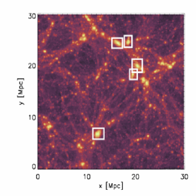
Figure 1: Projection of a simulation with $256^{3}$ particles. The boxes are the minimum size boxes of the five most massive halos found with FOF with a linking length of $R_{\rm link}=1/\left[5\sqrt[3]{\bar{n}}\right]$. Note that the apparent overlap of the boxes is just a projection effect.

In Fig. 1 we show the projection of the simulation with $256^{3}$ particles in a box of length $L=20h^{-1}{\rm Mpc}$ at a redshift $z=1$ and a mass resolution of $\approx 4\times 10^{7}{\rm M}_{\odot}/h$. The boxes are the minimum size boxes of the five most massive structures in the simulation.

This rough analysis of structure enables one already to estimate the mass distribution in the simulation.

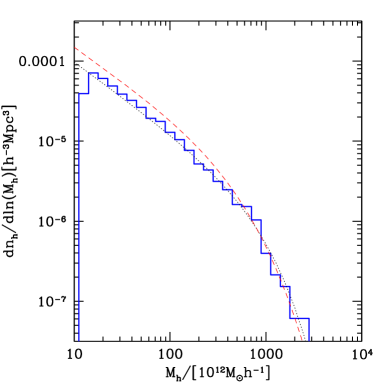
Figure 2: Mass function of clusters with more than 5000 particles for the $1024^{3}$ simulation (right). The dotted line is the Schechter function with a slope of $\alpha=0.9$ and exponential cut-off at a scale $M_{*}=8.0\times 10^{14}h^{-1}{\rm M}_{\odot}$. For comparison we also plot the mass function from Evrard et al. (2002) (dashed line).

In Fig. 2 we show the mass distribution of families for the $1024^{3}$ simulation described in Table 1. The dominance of low mass objects is clear. Also we show a fit to the slope of the distribution with to a generalised Schechter function (Press & Schechter, 1974; Schechter, 1976) $dn_{h}/dln(M_{h})=N_{*}(M_{h}/M_{*})^{-\alpha}\exp(-M_{h}/M_{*})$ and obtain $\alpha\approx 0.9$. The fit was performed with a nonlinear least-squares Marquadt-Levenberg algorithm. Note that at this stage we plot the mass function of the families, which makes it harder to compare with the standard Press-Schechter prescription, which assumes virial masses and does not take into account the linking of overlapping structures, however our findings are consistent with previous work (Ghigna et al., 2000). The dashed line in Figure 2 from shows the distribution measured by Evrard et al. (2002), which establishes that this rough catalog agrees well with standard expectations.

After this first step we have identified large structures in the simulation and assigned all particles which potentially belong to these structures. This will enable us in the next step to refine the analysis within a single family.

2.2 Identification of substructure and bound particles in halos

We are now in the position to study a single family in more detail. We first perform an identification of groups within one family using the Denmax algorithm (Bertschinger & Gelb, 1991; Gelb & Bertschinger, 1994). Denmax first interpolates the density field $\rho$ by applying a Gaussian kernel with a given smoothing length $R_{\rm smooth}$ to the particle positions. The particles are then shifted along the density gradient via the fluid equation

$$\frac{d{\mathbf{x}}}{d\tau}={\mathbf{\nabla}}\frac{\delta\rho}{\rho}\,.$$ (1)

Each particle moves toward a density maximum where it comes to rest, or more probably oscillates around the peak. The groups are then identified by using the FOF scheme on the shifted particles, with a linking length comparable to $R_{\rm smooth}$. We use a much smaller smoothing length $R_{\rm smooth}$ than the linking length $R_{\rm link}$ in the FOF scheme used previously for finding the rough structures. We take

$$R_{\rm smooth}=f_{\rm sub}\epsilon\,,$$ (2)

where $\epsilon$ is the softening length of the simulation and $f_{\rm sub}$ is a free parameter in our analysis, which we typically choose to be $f_{\rm sub}=5$. This choice ensures that we identify the smallest structures which are still above the resolution threshold of the simulation (Ghigna et al., 2000). We also set the threshold for the minimum number of particles in a group to 10. In this way we obtain a list of groups within the single family.

After the refined Denmax step there are still particles which are not assigned to any group with more than 10 particles. For each such particle, we locate the nearest neighbour structures and calculate the distance $\delta r$ to their density peak positions. We also calculate the distance to the peak of the most massive group, which we call the mother halo. We then calculate $m/\delta r^{2}$, where $m$ is the mass of the neighbour, and assign the particle to the group (or the mother) where this quantity is maximal. We note that any mis-assignments made at this stage will be rectified at a later stage in the analysis, and the purpose of this simple criterion is to minimise the necessary amount of reassignment.

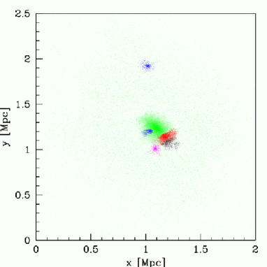
Figure 3: Projection of all particles in the mother halo (background), and the five most massive substructures found by the refined Denmax run. The cluster has a total mass of $1.3\times 10^{13}h^{-1}{\rm M}_{\odot}$ and the substructures range between $1.2\times 10^{9}h^{-1}{\rm M}_{\odot}$ and $2.3\times 10^{11}h^{-1}{\rm M}_{\odot}$ for this simulation.

As an example, we show in Fig. 3 the five most massive substructures identified in the most massive mother halo of the $256^{3}$ simulation, which has initially $\approx 321,000$ particles, or a mass of $1.3\times 10^{13}h^{-1}{\rm M}_{\odot}$. The masses of all the substructures vary between $1.2\times 10^{9}h^{-1}{\rm M}_{\odot}$ and $2.3\times 10^{11}h^{-1}{\rm M}_{\odot}$, where we assume we can reliably identify a substructure if it comprises of at least 30 particles.

The next step is the build up of the family tree within this family. In order to obtain the family tree, we calculate the minimum size box which contains each identified substructure. Then, as before, we apply a bottom–up scheme starting with the lowest mass halo and determine if its density peak is within the minimal box enclosing a more massive structure. The structure with the lowest mass which contains the halo is identified to be the mother of this halo, while the halo becomes the daughter and hence a substructure of the mother. If the density peak is not within any other halo, we check if the minimal box is overlapping with any other box. In this case we take the lowest mass overlap halo as the mother. We then move to the next more massive halo and repeat the procedure. Once we have identified the mother, all the substructures of the daughter will also become daughters of the mother. In this way we obtain a unique mother for each halo, and for each mother a list of daughters which contains all substructures of the hierarchy. We should actually talk of daughters, grand-daughters, great grand-daughters and so on, but there is no need to distinguish daughters and grand-daughters from a mother’s point of view, as long as each daughter knows who her mother is— which is ensured by our procedure. In other words, each mother knows about the whole younger generation, but only her mother from among her ancestors. “Isolated” substructures will have the original mother halo as a mother.

Figure 4: Schematic description of the family tree. Halo number 1 counts all subhalos 2 through 9 as her daughters. Halo 1 is the mother of subhalos 2, 3, and 4. Subhalos 5, 6, and 7 are also the daughters of subhalo 3, and see 3 as their mother; 7 and 8 are in a similar relation to subhalo 2. Number 4 is an isolated subhalo.

In Fig. 4 we show schematically the build up of a family tree.

We further introduce a threshold particle number $N_{t}$. Structures with fewer particles than $N_{t}$ are dissolved into their associated mothers. Typically we choose $N_{t}=30$, discarding smaller groups found earlier. In Ghigna et al. (2000) a threshold of $N_{t}=16$ has been used for using halos as tracers, but $N_{t}=32$ for the reliable analysis of properties of halos. However Diemand et al. (2004) find that the results are only stable for $N_{t}=100$. This is necessary to resolve a complete sample of subhalos.

 

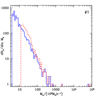
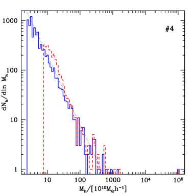
Figure 5: Left: Mass function of the substructures of the most massive halo of the $256^{3}$ simulation, before (solid line) and after (dashed line) structures with less than $N_{\rm t}=30$ have been dissolved into their mothers. The mother halo has $\approx 160,000$ particles or a mass of $6.5\times 10^{12}h^{-1}{\rm M}_{\odot}$. The dotted line is from a power law $dN_{h}/dln(M_{h})\propto M_{h}^{-1.4}$. Right: The same plot for the 4th most massive halo of the $1024^{3}$ simulation with $\approx 392,000$ particles and a mass of $1.1\times 10^{15}h^{-1}{\rm M}_{\odot}$ in the mother halo.

In Fig. 5 we show the distribution of substructures masses in the most massive halo of the $256^{3}$ run, and in the 4th most massive halo from the $1024^{3}$ simulation. In the following we call these halos cluster #1 (left) and cluster #4 (right). The entire structure, including the mother halo and all daughters, has a mass of $1.3\times 10^{13}h^{-1}{\rm M}_{\odot}$ for cluster #1 and $1.6\times 10^{15}h^{-1}{\rm M}_{\odot}$ for cluster #4. We clearly see the large number of small structures (solid lines); the original distribution follows roughly a scaling of $dN_{h}/dln(M_{h})\propto M_{h}^{-1.4}$ (dotted lines). This becomes even steeper if the halos with less than $N_{\rm t}=30$ particles are dissolved into their mothers (dashed lines). The Denmax routine had originally recovered about $5100$ substructures which have more than ten particles within cluster #1, and $7760$ halos within cluster #4. About 20-25% of the total mass of the structure is in halos with less than $30$ particles as identified by Denmax. After halos with less than $30$ particles have been dissolved into their mothers we are left with about $1790$ substructures in cluster #1 and 2590 in cluster #4. During this procedure the original mother halo gained $5.7\times 10^{11}h^{-1}{\rm M}_{\odot}$ for cluster #1 and $6.4\times 10^{13}h^{-1}{\rm M}_{\odot}$ for halo #4. The rest of the mass is distributed among the lower mass halos, as seen in the dashed histograms in Fig. 5.

As mentioned in the introduction, Denmax itself has been applied in a hierarchical way, either as part of SKID by applying three different smoothing lengths $l_{\rm link}=1.5,5,10l_{\rm soft}$ (Ghigna et al., 2000), or by using it on larger scales with $R_{\rm smooth}=0.2{\bar{n}}^{-1/3}$ and re-analysing each halo with $R_{\rm smooth}=0.1{\bar{n}}^{-1/3}$ (Neyrinck et al., 2004). The reason for this is that in general there is no single smoothing length which is suited to find structures over a large mass range in the simulation. If the smoothing length is too large then small structures are not resolved, and if it is too small then large structures are broken up. We choose a small smoothing length and recombine larger objects using the family tree hierarchy.

We have now a clearly defined, geometrically based picture of substructures, which we can proceed to analyse in a more physical fashion so that unbound particles are culled out. In some situations the Denmax procedure may err in assigning some particles to substructures. Imagine a particle which is dynamically a part of the mother halo: the Denmax algorithm will move this particle toward the cluster centre, but if a significant substructure just happens to intervene, the particle will reach this local maximum and stop. Thus there will be particles extending in a radial wedge outside of any bound structure arbitrarily attached to it, even if they are gravitationally not bound to it. To correct for such unphysical identifications, we need now a post–identification dynamical treatment of the halos.

2.2.1 Velocity outliers

It can be shown (Binney & Tremaine, 1987) that the rms escape velocity from a finite, bound self-gravitating system is related to the rms velocity by $\left<v^{2}_{\rm esc}\right>=4v_{\rm rms}^{2}$. Thus particles having a velocity greater than $\sqrt{2\left<v_{\rm esc}^{2}\right>}=\sqrt{8}v_{\rm rms}$ are very unlikely to be bound to the structure. One way to calculate the escape velocity is by measuring the maximum value of the circular velocity $v_{\rm circ}(r)=\sqrt{GM(r)/r}$; by assuming an NFW profile this can be related to the escape velocity (Klypin et al., 1999). However this method relies on the NFW profile which we do not want to assume at this stage.

To remove unbound particles from a substructure, we will instead proceed with a first approximation by calculating the typical rms velocity and removing particles which are statistical outliers. But we cannot calculate the velocity dispersion until we know the true centre of mass (CoM) velocity, so— because we have not removed unbound particles from the structure— we must proceed iteratively, beginning with an approximation for the CoM. We choose the density peak of the substructure (not including its daughters) as a first approximation to the CoM. In order to obtain the CoM velocity we calculate the median of the velocity of the $N_{v}=100$ nearest neighbours to the density peak within the structure. If the number of particles is less than 30, we take half the particles of the structure. In order to obtain a valid answer we must pay attention to binaries, which could bias the result to large velocities. Hence we identify binaries by searching the whole simulation for bound pairs. We so far have not found bound pairs of particles in all the simulations we studied, which also provides evidence that the simulation is not over-resolved. If we did find a bound pair, the two particles would be replaced by a single particle with twice the mass, and the CoM position and CoM velocity of the pair. This ensures that we do not encounter velocity biases due to binaries. We then can proceed to calculate the rms velocity $v_{\rm rms}^{2}=\left<\left({\mathbf{v}}_{\rm part}-{\mathbf{v}}_{\rm cm}\right)^{2}\right>$ for the $N_{v}=100$ particles around the density peak. All particles in the substructure which have a velocity

$${\mathbf{v}}_{\rm part}^{2}>f_{{\rm cut}}v_{\rm rms}^{2}\,,$$ (3)

are then removed and added to their associated mother structure. We iterate this process until the mass change of the substructure is less then $5\%$. We perform this velocity cut at two levels: first we use $f_{{\rm cut}}=8$ as noted earlier, and as mentioned above $N_{v}=100$ particles for the CoM velocity and rms velocity calculation. Then choosing a tighter limit with $f_{\rm cut}=6$, we find the centre of mass mean velocity and velocity dispersion of the inner half of the particles and repeat the process.

 

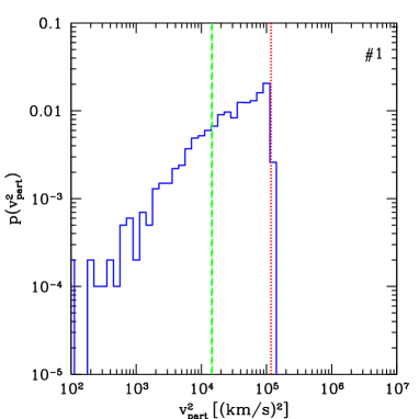
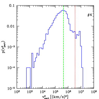
Figure 6: Distribution of the particle velocities in the most massive substructure, the velocity threshold $8v_{\rm rms}^{2}$ (dotted) and the rms velocity (dashed). All the particles above the threshold are moved to the associated mother. Cluster #1 is on the left, and #4 on the right.

In Fig. 6 we show the velocity distributions of the particles in the most massive substructure (solid line) in clusters #1 and #4. We also show the threshold rms velocity (dotted line) during the first step of the iteration. All particles above this threshold are moved to the associated mother. The mass of the mother halo at the end of this procedure increases just by $4.2\times 10^{11}h^{-1}{\rm M}_{\odot}$ for cluster #1 and $2.0\times 10^{13}h^{-1}{\rm M}_{\odot}$ for cluster #4, where most of the change occurs during the first cut-off scheme. After the removal of the velocity outliers we again dissolve halos with less than $N_{t}=30$ particles into their mothers.

At the end of this step we recalculate the CoM and $v_{\rm rms}$ for the subhalo and then we move daughters which have a faster CoM velocity than $\sqrt{6}v_{\rm rms}$ to the associated mother of the substructure under consideration.

2.2.2 Tree calculation of potentials and bound particles

We now reach the step where we can remove particles which have a total energy larger than zero in the centre of mass frame of the structure to which they belong. We will check within each substructure which particles are bound to it. We calculate the CoM of a substructure including all its daughters and compute the potential $\phi$ of the particles within the substructure. The potential calculation is done using an adaption of a tree code by Hernquist (1987). Note that we switch to an exact direct summation of of the potential energy if there are less than 100 particles in the system. The total energy of a particle is then

$$E_{\rm tot}=m\phi+\frac{1}{2}m\left({\mathbf{v}}_{\rm part}-{\mathbf{v}}_{\rm cm}\right)^{2}\;,$$ (4)

where $m$ is the mass of a particle, $\phi$ the potential from all the other masses within the substructure, and ${\mathbf{v}}_{\rm cm}$ the CoM velocity of the substructure. We calculate $E_{\rm tot}$ for each particle and then remove the third of the unbound particles with the highest energies, moving them to their associated mother structure. Note that we choose only a third of the particles because otherwise particles are removed to quickly without taking into account that the CoM velocity, and hence the kinetic energy, is changing with each removed particle. Ideally one should remove only one particle at a time, as it is done in SKID (Stadel et al., 1997), but this is too time consuming for hundreds of halos with over $10^{5}$ particles. We tested different fractions and observed that one third was the largest number which results in a stable result. We then recalculate the CoM and iterate this step until there is no change in the mass of the system.

 

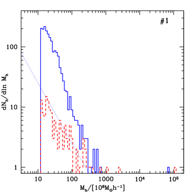
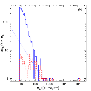
Figure 7: Mass function of substructure in the test clusters #1 (left) and #4 (right) after particles with high velocities have been moved to the associated mothers (solid line) and after unbound particles have been moved to the mother structure (dashed line). Note that the power laws are now $dN_{h}/dln(M_{h})\propto M_{h}^{-1.0}$ for #1 and $dN_{h}/dln(M_{h})\propto M_{h}^{-0.8}$ for #4.

In Fig. 7 we show the mass distribution before and after unbound particles have been moved to the mother structures. Note that all daughters with less than $N_{\rm t}=30$ particles have been dissolved into their mothers. There are many unbound particles in the substructures which returned to the original mother. The mother in halo #1 now has a mass of $1.2\times 10^{13}h^{-1}{\rm M}_{\odot}$ which corresponds to $\approx 293,000$ particles; there are now only $134$ daughters with a total mass of $1.1\times 10^{12}h^{-1}{\rm M}_{\odot}$. The mother of halo #4 has a mass of $1.5\times 10^{15}h^{-1}{\rm M}_{\odot}$ or $582,000$ particles, with $1.2\times 10^{14}h^{-1}{\rm M}_{\odot}$ remaining in $106$ daughters.

Before we proceed with the next step we will remove any daughter which is not bound to its mother. We approximate the potential energy for the daughters by

$$E_{\rm pot}^{\rm d}=-G\frac{m_{\rm d}M(r_{\rm d})}{r_{\rm d}}-G\int_{r_{d}}^{\infty}\frac{m_{\rm d}}{r}\;dM(r)\,,$$ (5)

where $m_{\rm d}$ is the daughter mass, $r_{\rm d}$ is the distance of the CoM of the daughter to the CoM of its mother, and $M(r)$ is the total mass of the mother within radius $r$ including all other daughters. We then can calculate the kinetic energy of the daughter with respect to the centre of mass its mother. If the daughter is not bound to her mother we move her to the mother of the mother.

2.2.3 Search for Hyper-structures

In order to obtain a stable algorithm with respect to the smoothing length for the refined Denmax procedure, we need, as noted above, to look for “hyper-structures”, groups of substructures which are gravitationally collectively bound to one another.

This problem has been addressed previously by combining the SKID algorithm with an adaptive FOF analysis (Diemand et al., 2004); we will take a different approach here. In order to do this we investigate primary substructures, ie. structures which are direct daughters of the largest structure which is the mother structure. For each such primary substructure, we calculate the distance $\delta r_{i}$ to each other primary substructure with mass $m_{i}$, and examine the one with the maximal $m_{i}/\delta r_{i}^{3}$ as follows; note that the masses include all daughters of the primary substructures. If these two structures are bound with respect to their common CoM, they form a hyper-structure; the less massive of the two becomes a daughter of the more massive structure. We than re-calculate the CoM and the maximum extension box of the new hyper-structure, and check each particle of the mother within this box. If it is bound to the hyper-structure, we then move it from the mother to this hyper-structure. We will iterate this step three times. Note that for both halos the mass in the mother structure does not change significantly during this step.

In this fashion bound objects, whose identity is independent of the geometrical tool used to analyse substructure, are assembled.

2.2.4 Final Steps: Daughters and Particles unbound to Entire Family

The next step we perform is to remove daughters which are not bound to the biggest structure, the mother halo. And finally we remove particles which are not bound to the family tree at all. For both halos none of the daughters is unbound and the number of unbound particles is negligible.

 

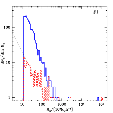
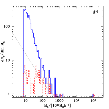
Figure 8: Mass function of substructures in the halo after the refined Denmax run and the mass cut (solid), and at the end of the the iterative scheme (dashed). The dotted lines show the power laws $dN_{h}/dln(M_{h})\propto M_{h}^{-1.1}$ (left) and $M_{h}^{-0.8}$ (right).

In Fig. 8 we show the mass distribution from the refined Denmax run (solid line) and after the unbinding steps (dashed line). There remains 8.8% of the mass in substructures for #1 (left) and 7.4% for halo #4 (right). For cluster #1 $dN_{h}/dln(M_{h})\propto M_{h}^{-1.1}$ for small mass halos, the distribution in cluster #4 is roughly approximated by $dN_{h}/dln(M_{h})\propto M_{h}^{-0.8}$. Note these are only rough power laws.

2.2.5 Truncation of Halo at the “virial radius” and Identification of Companions

Now we check if we have artificially linked together separate structures which are only weakly coupled together gravitationally, and if we have artificially included distant in-falling matter. For a $\Lambda$CDM cosmology, it is conventional to define the virial mass $M_{\rm vir}$ and radius $R_{\rm vir}$ with

$$M_{\rm vir}=\frac{4}{3}\pi R_{\rm vir}^{3}\Delta_{c}(z)\rho_{c}(z)\,,$$ (6)

where $\rho_{c}$ is the critical density of the universe, and the mean over-density $\Delta_{c}=178\Omega_{\rm m}(z)^{0.45}$. Thus we make a rank ordered list of our mother halos, and in each one we start at the density maximum and proceed outward until we reach the virial radius, within which the mean over-density is $\Delta_{c}$. We truncate the halo at this point, removing all particles from outside the virial radius of the halo and identifying daughters with centres outside this radius as separate companion structures. In this step the mass of the mother halo in cluster #1 stays almost constant at $1.1\times 10^{13}h^{-1}{\rm M}_{\odot}$ while 96 subhalos with a total mass of $9.4\times 10^{11}h^{-1}{\rm M}_{\odot}$ remain. In cluster #4 the mother mass is reduced to $1.2\times 10^{15}h^{-1}{\rm M}_{\odot}$ with 65 remaining subhalos of a mass of $8.2\times 10^{13}h^{-1}{\rm M}_{\odot}$.

 

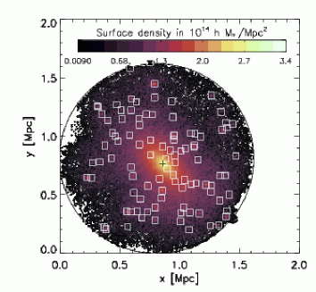
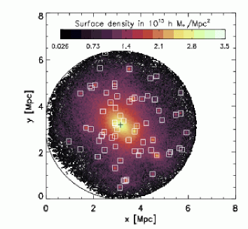
Figure 9: Particles and daughters in halo # 1 (left) and halo # 4 (right) after the cleanup procedure and removal of particles and subhalos outside the virial radius. The dark cross marks the centre of the halo and the boxes the identified and bound daughters. The colour corresponds to the surface density as indicated by the colour bar. Cluster #1 has 96 subhalos and #4 has 65.

In Fig. 9 we show the projected density inside the virial radius of cluster #1 (left) and cluster #4 (right), with the daughters marked. Note that cluster #1 is at a redshift of $z=1$ while cluster #4 at redshift $z=0.05$. Halo #1 has a virial radius of $r_{\rm vir}\approx 0.81\,{\rm Mpc}$ and halo #4 a radius of $r_{\rm vir}\approx 3.0\,{\rm Mpc}$. Note that for halo #4 the substructure is much more centered around the core than for halo #1.

3 Dependence on Parameters and Test of stability

In this section we discuss the stability of our method, as different possible choices of the parameters and procedures may affect the results.

3.1 Group Finding

We will first vary the linking length in our rough initial FOF analysis in order to establish how sensitive we are to this parameter choice. We perform an analysis with a linking length of $R_{\rm link}=0.167{\bar{n}}^{-1/3}$; this could potentially lead to a larger fragmentation of initial halos and families and hence potentially change our results. We find that the results of this run are almost identical with results obtained with the original linking length. For halo #4 we have after the initial fine Denmax run $35\%$ of the mass in substructures (compared to 34% in the original run) which is lowered to $9\%$ (8%) after we test for bound particles; after the final virial cut, $8\%$ of the halo mass in substructures while the original run resulted in slightly lower than $8\%$. This is due to the fact that our family tree procedure followed by a refined Denmax run produces almost the same large structures.

We did a further consistency check where instead of FOF we used a rough Denmax run with a smoothing length of $R_{\rm smooth}=1/5{\bar{n}}^{-1/3}$ to identify the initial halo list. The results were essentially the same as in the original runs. Hence we conclude that our method is stable with respect to sensible changes in the initial halo finding algorithm to within $\pm 1\%$, which is well below the statistical fluctuation of the sample.

The next halo finding step we perform is the refined Denmax run. We crucially chose in this step the smallest sensible smoothing length and then built up the halo hierarchy by our family tree algorithm. Making the smoothing length smaller than $R_{\rm smooth}=5\epsilon$ would enter the regime dominated by uncertainties in the force softening, so we do not extend a stability test in this direction.

Instead we repeated the analysis with a smoothing length of $R_{\rm smooth}=10\epsilon$. Due to the larger smoothing length, we find $56\%$ of the mass in substructures after the initial denmax step for halo #4; however, when we test for particles which are actually bound to these structures we obtain already $9\%$ of the mass in substructures. After the inclusion of hyper-structures and the density cut this drops to 7%, which is in excellent agreement compared to the run with a smoothing length $R_{\rm smooth}=5\epsilon$ ($8\%$).

We hence conclude that we have a reasonably stable criterion if the smoothing length is chosen within a reasonable range. Of course, as the smoothing length is made larger we will miss more and more structures.

3.2 Removal of unbound particles

The first step of removing unbound particles is performed by removing velocity outliers in a gentle way. Since we do this already in two steps with first a gentler and then a harder cut-off at $8v_{\rm rms}^{2}$ and $6v_{\rm rms}^{2}$ we established that most of the cut is happening during the first iteration step. However the velocity cut does not change the mass fraction significantly. Final results do not depend on the specific numbers $(8,6)\times v_{\rm rms}^{2}$, as long as we approach the final cut gradually. Furthermore, we note that this cut was mainly done to avoid an unphysical bias toward large CoM velocities, which is important for the calculation of the kinetic energies with respect to the centre of mass.

3.3 Virial Cut

Since the definition of a mass or size of a halo is to some extent arbitrary (see for example: Jenkins et al. (2001); Evrard et al. (2002); White (2002)), we will investigate how this definition influences our results. We chose initially the virial mass and radius corresponding in a $\Lambda$CDM cosmology to the over-density $\Delta_{c}(z)=178\Omega_{\rm m}(z)^{0.45}$. We saw already in the comparison of the $256^{3}$ and $1024^{3}$ simulations that, after this density cut, the fraction of mass in substructures can be quite different. However, the simulation with $256^{3}$ was also at a redshift of $z=1$, compared to $z=0$ for the $1024^{3}$ simulation. Hence we performed an analysis of the the $1024^{3}$ run where we chose the cut-off over-density to be $\Delta_{c}=200$ in agreement with another commonly used definition. With this cut-off the final mass-fraction in subhalos only decreases from $8\%$ to $7\%$ for halo $\#4$.

4 Application to a Different Simulation

In order to test our algorithm we applied it to a simulation provided by Diemand et al. (2004). We chose their cluster $D6$, where the simulation was done with a smoothing length of $\epsilon=3.6\,{\rm kpc}$, which is comparable to our runs. Diemand et al. (2004) state that their halo finding is complete for halos with more than 100 particles and they find about 5% of the mass in substructures. We also obtain with our scheme 5% of the mass in substructures, which is excellent agreement given the difference of the analysis methods. Diemand et al. (2004) use a hierarchical version of the SKID algorithm which is based on DENMAX. They perform the unbinding iteratively and exactly with no approximation like the one discussed in Section 2.2.

In order to get a further inside into the statistics of substructures we compare the cumulative massfunctions of halo $D6$ from our analysis and the analysis by Diemand et al. (2004).

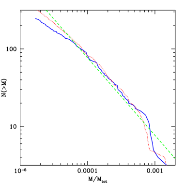
Figure 10: Cumulative mass function for substructures with more than $30$ particles in halo $D6$ as presented by Diemand et al. (2004). The solid line is from the algorithm presented here, the dotted line from (Diemand et al., 2004) and the dashed line has a slope of $M^{-1}$.

In Fig. 10 we show the cumulative mass function for substructures in the test halo $D6$. The solid line is from our analysis and the dashed line from (Diemand et al., 2004). They look both very similar and scale very closely to $M^{-1}$ until a cut-off at less than a thousandth of the total cluster mass. Our analysis results in slightly more substructures than the one of (Diemand et al., 2004). We find 272 substructure while they find 241. This is actually strikingly similar given the difference of the presented algorithms and the overall mass fraction in substructures for both analysis is at the 5% level within 1% uncertainty.

5 Conclusion

In this paper we have established a fast and stable algorithm to identify vast numbers of substructures in large N-body simulations in a speedy fashion. For example to analyse the most massive halo of about 1.5 million particles takes about 8 hours on a SUN BLADE 2000 on a single 900 MHz processor with 3 Gbyte RAM. We established an approximate method to identify and remove unbound particles from subhalos, which allows for the efficient calculation of bound structures. We analysed three simulations, two done by the TPM code developed by Bode et al. (2000) and one by Diemand et al. (2004). For all three we find similar mass fractions of about 5-8%. (Diemand et al., 2004) find about 5% of the mass in substructures, which is identical with our findings.

The fraction of substructure in a cold dark matter cluster is to some extend a question of definition. If one for instance is interested in strong lensing, which tests the distribution of matter, the question of bound or unbound structures is irrelevant. However, if substructures are the places where galaxies form, a full dynamical treatment is relevant and requires the inclusion of all forces, including the ones from internal and external potential.

To conclude we emphasize that the presented algorithm is stable and fast and ready to be employed for large cosmological data sets as well as detailed simulations of clusters of galaxies.

References

- Bertschinger & Gelb (1991) Bertschinger E., Gelb J., 1991, Comp. Phys., 5, 164
- Binney & Tremaine (1987) Binney J., Tremaine S., 1987, Galactic Dynamics. Princeton University Press, Princeton, NJ, USA
- Bode et al. (2001) Bode P., Ostriker J., Turok N., 2001, ApJ, 556, 93
- Bode & Ostriker (2003) Bode P., Ostriker J. P., 2003, ApJS, 145, 1B
- Bode et al. (2000) Bode P., Ostriker J. P., Xu G., 2000, ApJS, 128, 561
- Davis et al. (1985) Davis M., Efstathiou G., Frenk C. S., White S. D. M., 1985, Ap. J., 292, 371
- De Lucia et al. (2004) De Lucia G., Kauffmann G., Springel V., White S. D. M., Lanzoni B., Stoehr F., Tormen G., Yoshida N., 2004, MNRAS, 348, 333
- Diemand et al. (2004) Diemand J., Moore B., Stadel J., 2004, MNRAS, 352, 535
- Eisenstein & Hut (1998) Eisenstein D., Hut P., 1998, Ap. J., 498, 137
- Evrard et al. (2002) Evrard A. E., et al., 2002, Ap. J., 573, 7
- Evrard et al. (2002) Evrard A. E., MacFarland T. J., Couchman H. M. P., Colberg J. M., Yoshida N., White S. D. M., Jenkins A., Frenk C. S., Pearce F. R., Peacock J. A., Thomas P. A., 2002, Ap. J., 573, 7
- Gelb & Bertschinger (1994) Gelb J., Bertschinger E., 1994, Ap. J., 436, 467
- Ghigna et al. (2000) Ghigna S., et al., 2000, Ap. J., 544, 616
- Ghigna et al. (1998) Ghigna S., Moore B., Governato F., Lake G., Quinn T., Stadel J., 1998, MNRAS, 300, 146
- Gill et al. (2004) Gill S. P. D., Knebe A., Gibson B. K., 2004, astro-ph/0404258
- Gnedin et al. (1999) Gnedin O. Y., Hernquist L., Ostriker J. P., 1999, Ap. J., 514, 109
- Huchra & Geller (1982) Huchra J., Geller M., 1982, Ap. J., 257, 423
- Jenkins et al. (2001) Jenkins A., Frenk C. S., White S. D. M., Colberg J. M., Cole S., Evrard A. E., Couchman H. M. P., Yoshida N., 2001, MNRAS, 321, 372
- Kim & Park (2004) Kim J., Park C., 2004, astro-ph/0401386
- Klypin et al. (1999) Klypin A., Gottlöber S., Kravtsov A. V., Khokhlov A. M., 1999, Ap. J., 516, 530
- Kravtsov et al. (2003) Kravtsov A. V., et al., 2003, astro-ph/0308519
- Lacey & Cole (1994) Lacey C., Cole S., 1994, MNRAS, 271, 676
- Moore et al. (1999) Moore B., Ghigna S., Governato F., Lake G., Quinn T., Stadel J., Tozzi P., 1999, ApJL, 524, L19
- Moore et al. (1996) Moore B., Katz N., Lake G., 1996, Ap. J., 457, 455
- Navarro et al. (1995) Navarro J., Frenk C., White S. D. M., 1995, MNRAS, 275, 720
- Neyrinck et al. (2004) Neyrinck M. C., Gnedin N. Y., Hamilton A. J. S., 2004, astro-ph/0402346
- Neyrinck et al. (2004) Neyrinck M. C., Hamilton A. J. S., Gnedin N. Y., 2004, MNRAS, 348, 1
- Okamoto & Habe (1999) Okamoto T., Habe A., 1999, Ap. J., 516, 591
- Press & Schechter (1974) Press W., Schechter P., 1974, Ap. J., 187, 452
- Schechter (1976) Schechter P., 1976, Ap. J., 203, 297
- Springel et al. (2001) Springel V., White S. D. M., Tormen G., Kauffmann G., 2001, MNRAS, 328, 726
- Stadel et al. (1997) Stadel J., Katz N., Weinberg D. H., Hernquist L., 1997, www-hpcc.astro.washington.edu/tools/skid.html
- Summers et al. (1995) Summers F. J., Davis M., Evrard A., 1995, Ap. J., 454, 1
- van Kampen (1995) van Kampen E., 1995, MNRAS, 273, 295
- Warren et al. (1992) Warren M., Quinn P., Salmon J., Zurek W., 1992, Ap. J., 399, 405
- Weinberg et al. (1997) Weinberg D., Hernquist L., Katz N., 1997, Ap. J., 477, 8
- White (2002) White M., 2002, ApJS, 143, 241
- White (1976) White S. D. M., 1976, MNRAS, 177, 717