Model independent analysis of dark energy: Supernova fitting result

Abstract

This paper uses the supernova data to explore the property of dark energy by some model independent methods. We first Taylor expand the scale factor $a(t)$ and the luminosity distance $d_{\rm L}$ to the fifth order to find out that the deceleration parameter $q_{0}<0$. This result just invokes the Robertson-Walker metric. So the conclusion that the universe is expanding with acceleration is more general. Then we discuss several different parametrizations used in the literature. We also proposed two modified parametrizations. We find that $\omega_{\rm DE0}$ is less than $-1$ almost at $1\sigma$ level from all the parametrizations used in this paper. We also find that the transition redshift from deceleration phase to acceleration phase is $z_{\rm T}\sim 0.3$.

1 Introduction

The type Ia supernova (SN Ia) observation suggests that dark energy contributes 2/3 to the critical density of the present universe [1, 2, 3]. SN Ia observation also provides the evidence of a decelerated universe in the recent past with the transition redshift $z_{\rm T}\sim 0.5$ [4, 5, 6]. The cosmic microwave background (CMB) observations favor a spatially flat universe as predicted by inflationary models [7, 8]. There are many dark energy models proposed in the literature. For a review of dark energy models, see, for example, [9] and [10] and references therein. However, the nature of dark energy is still unknown. It is not practical to test every single dark energy model by using the observational data. Therefore, a model independent probe of dark energy is one of the best ways to study the nature of dark energy.

The type Ia supernovae (SNe Ia) as standard candles are used to measure the luminosity distance-redshift relationship $d_{\rm L}(z)$. So we can model the luminosity distance $d_{\rm L}$ to study the property of dark energy. Melchiorri etal. first found that dark energy may be a phantom type by combining different observational data to probe the behaviour of dark energy [11]. Huterer and Turner modelled the luminosity distance by a simple power law $d_{\rm L}(z)=\sum_{i=1}^{N}c_{i}z^{i}$ [12]. Saini etal. used a more complicated function to model the luminosity distance [13]. Another way to probe the nature of dark energy is to parameterize the dark energy equation of state parameter $\omega_{\rm DE}$. The simplest parametrization is the constant equation of state model $\omega_{\rm DE}={\rm constant}$. Several authors modelled $\omega_{\rm DE}$ as $\omega_{\rm DE}=\sum_{i=0}^{N}\omega_{i}z^{i}$ [14, 15, 16]. Apparently this parametrization is not good for high $z$. Recently, a stable parametrization $\omega_{\rm DE}=\omega_{0}+\omega_{a}z/(1+z)$ was used in [17, 18, 19, 20]. By fitting the model to SN Ia data, we find that $\omega_{0}+\omega_{a}>0$, so this parametrization is not good at high $z$ too. Jassal, Bagla and Padmanabhan modified this parametrization as $\omega_{\rm DE}=\omega_{0}+\omega_{a}z/(1+z)^{2}$ and the problem was solved because $\omega_{\rm DE}=\omega_{0}$ at present and at high $z$ [21]. More complicated functional forms for $\omega_{\rm DE}(z)$ were also proposed in the literature [22, 23, 24, 25]. We can also model the dark energy density itself. For example, a simple power law expansion $\Omega_{\rm DE}=\sum_{i=0}^{N}A_{i}z^{i}$ was used to investigate the nature of dark energy [26, 27, 28, 29, 30, 31]. There are other parametrizations, like the piecewise constant parametrization [32, 33, 34, 35].

This paper is organized as follows. In section II, We first use a Taylor expansion to expand the scale factor, then we fit the model to the whole 157 gold sample of SNe Ia compiled by Riess etal. in [6]. By expanding the scale factor, the fitting parameters have physical meanings. In section III, we analyze the dark energy parametrization proposed by Alam etal. [26]. In section IV, we first study the parametrization $\omega_{\rm DE}=\omega_{0}+\omega_{a}z/(1+z)$ and point out that this parametrization is not good at high $z$. Then we study the parametrization $\omega_{\rm DE}=\omega_{0}+\omega_{a}z/(1+z)^{2}$. In section V, we first investigate the parametrization proposed by Wetterich [25], then we propose two modified parametrizations. In section VI, we give some discussions.

2 Model Independent Method

In a homogeneous and isotropic universe, the Friedmann-Robertson-Walker (FRW) space-time metric is

$$ds^{2}=-dt^{2}+a^{2}(t)\left[{dr^{2}\over 1-k\,r^{2}}+r^{2}\,d\Omega\right].$$ (1)

For a null geodesic, we have

$$\int_{t_{1}}^{t_{0}}{dt\over a(t)}=\int_{0}^{r_{1}}{dr\over\sqrt{1-kr^{2}}}\equiv f(r_{1}),$$ (2)

where

$$f(r_{1})=\left\{\begin{array}[]{ll}\sin^{-1}r_{1},&k=1,\\ r_{1},&k=0,\\ \sinh^{-1}r_{1},&k=-1.\end{array}\right.$$ (3)

From Eq. (2), we get the luminosity distance $d_{\rm L}=a_{0}(1+z)r_{1}$ by Taylor expansion [36],

$$H_{0}d_{\rm L} = z+{1\over 2}(1-q_{0})z^{2}+{1\over 6}(q_{0}+3q_{0}^{2}-1-j_{0}-\Omega_{k})z^{3}+{1\over 24}(2-2q_{0}-$$ (4)

$$15q_{0}^{2}-15q_{0}^{3}+5j_{0}+10q_{0}j_{0}+s_{0}+2\Omega_{k}+6\Omega_{k}q_{0})z^{4}+O(z^{5}),$$

where the redshift $z$ is defined as $1+z=a_{0}/a(t)$, the subscript 0 means that a variable is evaluated at the present time, the Hubble parameter $H(t)$, the deceleration parameter $q(t)$, the jerk parameter $j(t)$ and the snap parameter $s(t)$ are defined as

$$H(t)=\dot{a}/a={1\over a}{da\over dt},$$ (5)

$$q(t)=-a^{-1}H^{-2}\ddot{a}=-{1\over aH^{2}}{d^{2}a\over dt^{2}},$$ (6)

$$j(t)={1\over aH^{3}}{d^{3}a\over dt^{3}},$$ (7)

$$s(t)={1\over aH^{4}}{d^{4}a\over dt^{4}},$$ (8)

and $\Omega_{k}=k/(a^{2}_{0}H^{2}_{0})$. The use of jerk parameter is equivalent to the statefinder used in [37, 38]. We may use the above expression (4) to probe the geometry of the Universe [39, 40]. Note that the Taylor expansion of $d_{\rm L}$ may break down at high $z$ and the actual behaviour of $d_{\rm L}$ may not be represented by finite number of terms. It is also straightforward to get

$$H^{2}(z)=H^{2}_{0}[1+2(1+q_{0})z+(1+2q_{0}+j_{0})z^{2}-{1\over 3}(s_{0}+q_{0}j_{0})z^{3}+O(z^{4})],$$ (9)

$$q(z)=q_{0}-(q_{0}+2q_{0}^{2}-j_{0})z+\left(4q_{0}^{3}+4q_{0}^{2}+q_{0}-2j_{0}-{s_{0}\over 2}-{7j_{0}q_{0}\over 2}\right)z^{2}+O(z^{3}).$$ (10)

Now let us find out $q_{0}$, $j_{0}$ and $s_{0}$ from the SN Ia data compiled by Riess etal., These parameters are determined by minimizing

$$\chi^{2}=\sum_{i}{[\mu_{\rm obs}(z_{i})-\mu(z_{i})]^{2}\over\sigma^{2}_{i}},$$ (11)

where $\sigma_{i}$ is the total uncertainty in the SN Ia observation and the extinction-corrected distance modulus $\mu(z)=5\log_{10}(d_{\rm L}(z)/{\rm Mpc})+25$. In the fitting process, we use the SN Ia gold sample only and we consider a flat universe with $\Omega_{k}=0$. Because we use Taylor expansion to get the luminosity distance, this expansion may break down at high $z$. Therefore, we first use the full 157 gold sample SNe, then we use those 148 SNe with $z\leq 1.0$. The best fit parameters to the whole 157 gold sample SNe are ($q_{0}$, $j_{0}$, $s_{0}$)=($-1.1$, $6.4$, $39.5)$ with $\chi^{2}=174.2$. The best fit parameters to the 148 gold sample SNe with $z\leq 1.0$ are ($q_{0}$, $j_{0}$, $s_{0}$)=($-1.7$, $14.4$, $149.4)$ with $\chi^{2}=160.8$.

If we expand the luminosity distance $d_{\rm L}$ to the third order only, i.e., we only consider the parameters $q_{0}$ and $j_{0}$ in Eq. (4), then we find that the best fit parameters to the whole 157 gold sample SNe are: $q_{0}=-0.64^{+0.25}_{-0.26}$, $j_{0}=1.2^{+1.5}_{-1.1}$ and $\chi^{2}=176.1$. At 99.5% confidence level, $q_{0}=-0.64^{+0.56}_{-0.59}$, so we conclude that the expansion of the Universe is accelerating with 99.5% confidence. From Eq. (10), we get $z_{\rm T}=q_{0}/(q_{0}+2q_{0}^{2}-j_{0})=0.595_{-0.177}^{+1.849}$. The best fit parameters to the 148 gold sample SNe with $z\leq 1.0$ are: $q_{0}=-1.0\pm 0.4$, $j_{0}=4.7^{+4.1}_{-3.1}$ and $\chi^{2}=161.3$. At 99.5% confidence level, $q_{0}=-1.0^{+0.9}_{-1.0}$, so we conclude again that the expansion of the Universe is accelerating with 99.5% confidence. With the best fit parameters, we find that $z_{\rm T}=q_{0}/(q_{0}+2q_{0}^{2}-j_{0})=0.295_{-0.056}^{+0.174}$. The contour plot for $q_{0}$ and $j_{0}$ is shown in Figs. 1 and 2.

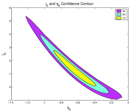
Figure 1: The plot of $q_{0}$ and $j_{0}$ contour fitting to the whole 157 gold sample SNe.

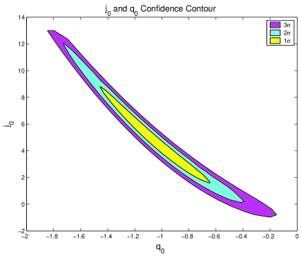
Figure 2: The plot of $q_{0}$ and $j_{0}$ contour fitting to the 148 gold sample SNe with $z\leq 1.0$.

So far our analysis uses the FRW metric only, we have not specified any gravitational theory yet. The above results are applicable to a wide range of theories. For example, $q_{0}=(\Omega_{\rm m0}-2\Omega_{\Lambda})/2$ and $j_{0}=\Omega_{\rm m0}+\Omega_{\Lambda}$ for the $\Lambda$-CDM model. If we expand the luminosity distance to the fifth order with the crackle parameter $c(t)=(aH^{5})^{-1}d^{5}a/dt^{5}$, then we need to add to Eq. (4) the following correction

$$-{1\over 120}(6+14q_{0}-61q^{2}_{0}-160q^{3}_{0}-105q^{4}_{0}+110q_{0}j_{0}$$

$$+105q^{2}_{0}j_{0}+15q_{0}s_{0}+27j_{0}-10j^{2}_{0}+11s_{0}+c_{0})z^{5}.$$ (12)

The best fit parameters to the whole 157 gold sample SNe are ($q_{0}$, $j_{0}$, $s_{0}$, $c_{0}$)=($-1.1$, $7.6$, $55.6$, 676.6) with $\chi^{2}=173.4$. The correction to $H_{0}d_{\rm L}$ at $z=1.5$ is about $-1.3$ which is around 34%. The best fit parameters to the 148 gold sample SNe with $z\leq 1.0$ are ($q_{0}$, $j_{0}$, $s_{0}$, $c_{0}$)=($-1.5$, $11.4$, $101.2$,$1484.2$) with $\chi^{2}=160.8$. The correction to $H_{0}d_{\rm L}$ at $z=1.5$ is about $0.19$ which is around 8.5%. Therefore the introduction of the fifth order correction changes the value of $q_{0}$ a little. We still have $q_{0}<0$. It is clear that the kinematic determination of the cosmological parameters is better suited for low redshift SNe Ia. However, from the observational data, $(z,\ \mu(z))=(1.4,\ 45.09)$, $(z,\ \mu(z))=(1.551,\ 45.3)$ and $(z,\ \mu(z))=(1.755,\ 45.53)$, we see that $\Delta\mu(z)=0.21$ when $\Delta z=0.151$ and $\Delta\mu(z)=0.23$ when $\Delta z=0.205$. Theoretically, we know that $d\mu(z)=(5/\ln(10))(d\,d_{\rm L}(z)/d_{\rm L}(z)dz)dz$. From Eq. (4), we get $d\mu(z)=(5/\ln(10))(n/z)dz$ if the luminosity distance is dominated by the higher term $z^{n}$. Combining the above analysis, we find that $n\sim 1$. Therefore, in this case, the higher term may not be the dominant term.

We conclude that $q_{0}<0$ with 99.5% confidence. In other words, we conclude that the Universe is expanding with acceleration.

3 ”Taylor expansion” of Dark Energy Density

In this section, we parameterize the dark energy density as [26]

$$\Omega_{\rm DE}(z)=A_{0}+A_{1}(1+z)+A_{2}(1+z)^{2},$$ (13)

where $\Omega_{\rm DE}(z)=8\pi G\rho_{\rm DE}(z)/(3H^{2}_{0})$, $\Omega_{\rm m0}=8\pi G\rho_{\rm m0}/(3H^{2}_{0})$ and $A_{0}=1-\Omega_{\rm m0}-A_{1}-A_{2}$. This parametrization is equivalent to Eq. (9) with $\Omega_{\rm m0}=-(s_{0}+q_{0}j_{0})/3$. The relationship between $\omega_{\rm DE}$ and $z$ is

$$\omega_{\rm DE}={1+z\over 3}{A_{1}+2A_{2}(1+z)\over A_{0}+A_{1}(1+z)+A_{2}(1+z)^{2}}-1.$$

With the above parameteriaztion, we find that $\Omega_{\rm DE}\ll\Omega_{m}$ and $\omega_{\rm DE}\approx-1/3$ when $z\gg 1$. Combining the above two equations, we find that the transition redshift $z_{\rm T}$ satisfies

$$\Omega_{\rm m0}(1+z)^{3}-A_{1}(1+z)-2A_{0}=0.$$ (14)

The best fit to the whole 157 gold sample SNe gives $A_{1}=-5.79$, $A_{2}=2.9$ and $\Omega_{\rm m0}\sim 0$ with $\chi^{2}=174.05$. If we use a Gaussian prior $\Omega_{\rm m0}=0.3\pm 0.04$ [41], then we get the best fit parameters $A_{1}=-4.2^{+4.6}_{-5.4}$ and $A_{2}=1.7^{+2.2}_{-1.8}$ with $\chi^{2}=174.21$. Substitute these parameter values to Eq. (14), we find that $z_{\rm T}=0.35$. The evolutions of the dark energy density and $\omega_{\rm DE}$ are shown in Fig. 3. Alam et al. showed that the SNe Ia data favored an evolving dark energy model by using the above reconstruction [26, 27]. They also showed that $z_{\rm T}\sim 0.4$. Our results are consistent with those analysis.

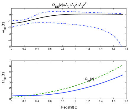
Figure 3: The best fit to the 157 gold sample SNe Ia with the prior $\Omega_{\rm m0}=0.3\pm 0.04$. The upper panel shows $\omega_{\rm DE}(z)$, the dotted dash lines are the 1$\sigma$ regions. The lower panel shows $\Omega_{\rm m}(z)$ and $\Omega_{\rm DE}(z)$

Because it is possible that $\omega_{\rm DE}<-1$, so we consider another two parameter representation of dark energy

$$\Omega_{\rm DE}(z)=B_{0}+B_{1}(1+z)+B_{-1}/(1+z),$$ (15)

where $B_{0}=1-\Omega_{\rm m0}-B_{1}-B_{-1}$. with this parametrization, we get

$$\omega_{\rm DE}={1\over 3}{B_{1}(1+z)^{2}-B_{-1}\over B_{1}(1+z)^{2}+B_{0}(1+z)+B_{-1}}-1.$$

The above equation tells us that $\Omega_{\rm DE}\ll\Omega_{m}$ and $\omega_{\rm DE}\approx-2/3$ when $z\gg 1$. Combining the above two equations, we find that the transition redshift $z_{\rm T}$ satisfies

$$\Omega_{\rm m0}(1+z)^{3}-B_{1}(1+z)-2B_{0}-{3B_{-1}\over 1+z}=0.$$ (16)

The best fit to the whole 157 gold sample SNe Ia gives $B_{-1}=6.87$, $B_{1}=6.14$ and $\Omega_{\rm m0}\sim 0$ with $\chi^{2}=173.2$. If we use a Gaussian prior $\Omega_{\rm m0}=0.3\pm 0.04$, then we get the best fit parameters $B_{-1}=4.1^{+4.7}_{-4.2}$ and $B_{1}=2.8^{+3.4}_{-3.0}$ with $\chi^{2}=173.65$. Substitute the best fit parameters into Eq. (16), we get $z_{\rm T}=0.30$. The evolutions of $\omega_{\rm DE}$ and $\Omega_{\rm DE}$ are shown in Fig. 4.

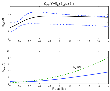
Figure 4: The best fit to the 157 gold sample SNe Ia with the prior $\Omega_{\rm m0}=0.3\pm 0.04$. The upper panel shows $\omega_{\rm DE}(z)$, the dotted dash lines are the 1$\sigma$ regions. The lower panel shows $\Omega_{\rm m}(z)$ and $\Omega_{\rm DE}(z)$

4 Stable Parametrization

In this section, we first consider the parametrization [17, 18]

$$\omega_{\rm DE}=\omega_{0}+{\omega_{a}z\over 1+z}.$$ (17)

When $z\gg 1$, we have $\omega_{\rm DE}\sim\omega_{0}+\omega_{a}$. The dark energy density is

$$\Omega_{\rm DE}=\Omega_{\rm DE0}(1+z)^{3(1+\omega_{0}+\omega_{a})}\exp(-3\omega_{a}z/(1+z)).$$

Combining the above two equations, we find that $z_{\rm T}$ satisfies

$$\Omega_{\rm m0}+(1-\Omega_{\rm m0})\left(1+3\omega_{0}+{3\omega_{a}z\over 1+z}\right)(1+z)^{3(\omega_{0}+\omega_{a})}\exp\left({-3\omega_{a}z\over 1+z}\right)=0.$$ (18)

The best fit to the whole 157 gold sample SNe Ia gives $\omega_{0}=-2.5$, $\omega_{a}=3.7$ and $\Omega_{\rm m0}=0.46$ with $\chi^{2}=173.5$. If we use a Gaussian prior $\Omega_{\rm m0}=0.3\pm 0.04$, then we get the best fit parameters $\omega_{0}=-1.6^{+0.6}_{-0.8}$ and $\omega_{a}=3.3^{+3.4}_{-3.7}$ with $\chi^{2}=173.92$. Substitute the best fit parameters into Eq. (18), we get $z_{\rm T}=0.35$. The evolutions of $\omega_{\rm DE}$ and $\Omega_{\rm DE}$ are shown in Fig. 5.

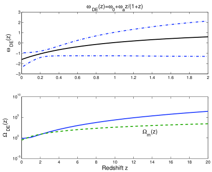
Figure 5: The best fit to the 157 gold sample SNe Ia with the prior $\Omega_{\rm m0}=0.3\pm 0.04$. The upper panel shows $\omega_{\rm DE}(z)$, the dotted dash lines are the 1$\sigma$ regions. The lower panel shows $\Omega_{\rm m}(z)$ and $\Omega_{\rm DE}(z)$

From Fig. 5, we see that the dark energy density is greater than the matter density at high $z$ because $\omega_{0}+\omega_{a}>0$. So this stable parametrization may not be a good choice at high $z$. Recently, Jassal, Bagla and Padmanabhan considered the following parametrization [21],

$$\omega_{\rm DE}=\omega_{0}+{\omega_{a}z\over(1+z)^{2}}.$$ (19)

When $z\gg 1$, we have $\omega_{\rm DE}\sim\omega_{0}$. The dark energy density is

$$\Omega_{\rm DE}=\Omega_{\rm DE0}(1+z)^{3(1+\omega_{0})}\exp(3\omega_{a}z^{2}/2(1+z)^{2}).$$

Combining the above two equations, we find that $z_{\rm T}$ satisfies

$$\Omega_{\rm m0}+(1-\Omega_{\rm m0})\left(1+3\omega_{0}+{3\omega_{a}z\over(1+z)^{2}}\right)(1+z)^{3\omega_{0}}\exp\left({3\omega_{a}z^{2}\over 2(1+z)^{2}}\right)=0.$$ (20)

The best fit to the whole 157 gold sample SNe Ia gives $\omega_{0}=-2.5$, $\omega_{a}=7.6$ and $\Omega_{\rm m0}=0.42$ with $\chi^{2}=173.3$. If we use a Gaussian prior $\Omega_{\rm m0}=0.3\pm 0.04$, then we get the best fit parameters $\omega_{0}=-1.9^{+0.9}_{-1.1}$ and $\omega_{a}=6.6\pm 6.7$ with $\chi^{2}=173.41$. Substitute the best fit parameters into Eq. (20), we get $z_{\rm T}=0.30$. The evolutions of $\omega_{\rm DE}$ and $\Omega_{\rm DE}$ are shown in Fig. 6.

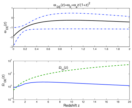
Figure 6: The best fit to the 157 gold sample SNe Ia with the prior $\Omega_{\rm m0}=0.3\pm 0.04$. The upper panel shows $\omega_{\rm DE}(z)$, the dotted dash lines are the 1$\sigma$ regions. The lower panel shows $\Omega_{\rm m}(z)$ and $\Omega_{\rm DE}(z)$

From Fig. 6, it is clear that the dark energy density did not dominate over the matter energy density at high $z$. Our result is consistent with that obtained in [21].

5 Wetterich’s Parametrization

In this section, we first consider the parametrization given in [25],

$$\omega_{\rm DE}={\omega_{0}\over[1+b\ln(1+z)]^{2}}.$$ (21)

When $z\gg 1$, we have $\omega_{\rm DE}\sim 0$. The dark energy density is

$$\Omega_{\rm DE}=\Omega_{\rm DE0}(1+z)^{3+3\omega_{0}/[1+b\ln(1+z)]}.$$

Combining the above two equations, we find that $z_{\rm T}$ satisfies

$$\Omega_{\rm m0}+(1-\Omega_{\rm m0})\left(1+{3\omega_{0}\over[1+b\ln(1+z)]^{2}}\right)(1+z)^{3\omega_{0}/[1+b\ln(1+z)]}=0.$$ (22)

The best fit to the whole 157 gold sample SNe Ia gives $\omega_{0}=-1.84$, $b=5.85$ and $\Omega_{\rm m0}\sim 0$ with $\chi^{2}=173.09$. If we use a Gaussian prior $\Omega_{\rm m0}=0.3\pm 0.04$, then we get the best fit parameters $\omega_{0}=-2.5^{+1.3}_{-4.8}$ and $b=4.0^{+11.4}_{-3.5}$ with $\chi^{2}=173.15$. Substitute the best fit parameters into Eq. (22), we get $z_{\rm T}=0.26$. The evolutions of $\omega_{\rm DE}$ and $\Omega_{\rm DE}$ are shown in Fig. 7.

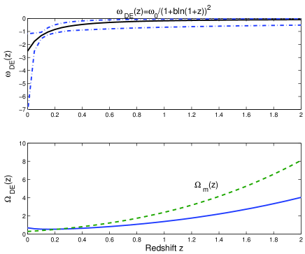
Figure 7: The best fit to the 157 gold sample SNe Ia with the prior $\Omega_{\rm m0}=0.3\pm 0.04$. The upper panel shows $\omega_{\rm DE}(z)$, the dotted dash lines are the 1$\sigma$ regions. The lower panel shows $\Omega_{\rm m}(z)$ and $\Omega_{\rm DE}(z)$

Because the best fit of the above parametrization gives $\Omega_{\rm m0}\sim 0$ which is not physical, we first modify the above parametrization as

$$\omega_{\rm DE}={\omega_{0}\over 1+b\ln(1+z)}.$$ (23)

When $z\gg 1$, we have $\omega_{\rm DE}\sim 0$. The dark energy density is

$$\Omega_{\rm DE}=\Omega_{\rm DE0}(1+z)^{3}[1+b\ln(1+z)]^{3\omega_{0}/b}.$$

Combining the above two equations, we find that $z_{\rm T}$ satisfies

$$\Omega_{\rm m0}+(1-\Omega_{\rm m0})\left(1+{3\omega_{0}\over 1+b\ln(1+z)}\right)\left[1+b\ln(1+z)\right]^{3\omega_{0}/b}=0.$$ (24)

The best fit to the whole 157 gold sample SNe Ia gives $\omega_{0}=-3.05$, $b=36.8$ and $\Omega_{\rm m0}\sim 0$ with $\chi^{2}=172.75$. If we use a Gaussian prior $\Omega_{\rm m0}=0.3\pm 0.04$, then we get the best fit parameters $\omega_{0}=-3.4^{+2.1}_{-17.7}$ and $\omega_{a}=17.8^{+162.3}_{-16.4}$ with $\chi^{2}=172.91$. This modification does not solve the problem of $\Omega_{\rm m0}\sim 0$. Substitute the best fit parameters into Eq. (24), we get $z_{\rm T}=0.25$. The evolutions of $\omega_{\rm DE}$ and $\Omega_{\rm DE}$ are shown in Fig. 8.

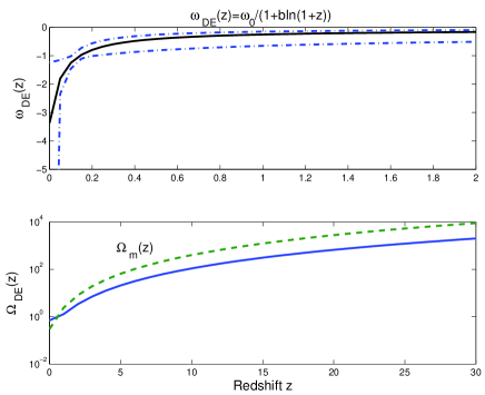
Figure 8: The best fit to the 157 gold sample SNe Ia with the prior $\Omega_{\rm m0}=0.3\pm 0.04$. The upper panel shows $\omega_{\rm DE}(z)$, the dotted dash lines are the 1$\sigma$ regions. The lower panel shows $\Omega_{\rm m}(z)$ and $\Omega_{\rm DE}(z)$

Now let us consider another modification

$$\omega_{\rm DE}=\omega_{0}+{\omega_{a}\over 1+\ln(1+z)}.$$ (25)

When $z\gg 1$, we have $\omega_{\rm DE}\sim\omega_{0}$. The dark energy density is

$$\Omega_{\rm DE}=\Omega_{\rm DE0}(1+z)^{3(1+\omega_{0})}[1+\ln(1+z)]^{3\omega_{a}}.$$

Combining the above two equations, we find that $z_{\rm T}$ satisfies

$$\Omega_{\rm m0}+(1-\Omega_{\rm m0})\left(1+3\omega_{0}+{3\omega_{a}\over 1+b\ln(1+z)}\right)(1+z)^{3\omega_{0}}[1+\ln(1+z)]^{3\omega_{a}}=0.$$ (26)

The best fit to the whole 157 gold sample SNe Ia gives $\omega_{0}=2.2$, $\omega_{a}=-4.7$ and $\Omega_{\rm m0}=0.454$ with $\chi^{2}=173.47$. If we use a Gaussian prior $\Omega_{\rm m0}=0.3\pm 0.04$, then we get the best fit parameters $\omega_{0}=2.4^{+2.6}_{-2.9}$ and $\omega_{a}=-4.1^{+3.4}_{-3.1}$ with $\chi^{2}=173.81$. Substitute the best fit parameters into Eq. (26), we get $z_{\rm T}=0.34$. The evolutions of $\omega_{\rm DE}$ and $\Omega_{\rm DE}$ are shown in Fig. 9.

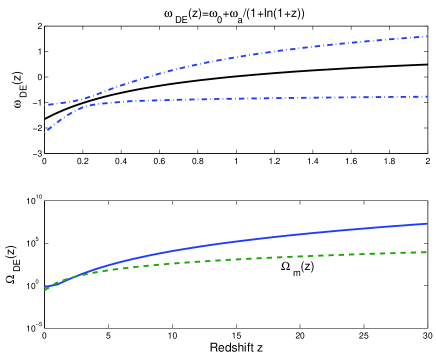
Figure 9: The best fit to the 157 gold sample SNe Ia with the prior $\Omega_{\rm m0}=0.3\pm 0.04$. The upper panel shows $\omega_{\rm DE}(z)$, the dotted dash lines are the 1$\sigma$ regions. The lower panel shows $\Omega_{\rm m}(z)$ and $\Omega_{\rm DE}(z)$

Although this modification solves the problem of $\Omega_{\rm m0}\sim 0$, it is not good at early times because the dark energy density dominated over the matter energy density at early times as shown in Fig. 9.

6 Discussions

The SN Ia data shows that the expansion of the Universe is accelerating. This conclusion derived from Eqs. (4) and (2) does not dependent on any particular model. We used the parametrizations (13), (15), (17), (19) and (21) proposed in the literature to discuss the property of dark energy. We also proposed two modified parametrizations (23) and (25). By using the above parametrizations, we derived the equations satisfied by the transition redshift. In order to see the property of $\omega_{\rm DE}(z)$, we re-plot $\omega_{\rm DE}(z)$ for all the models considered in this paper together in Fig. 10.

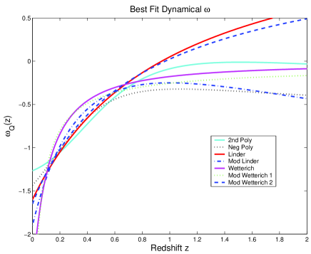
Figure 10: The evolution of $\omega_{\rm DE}$ for different parametrizations.

From Fig. 10, we see that: (a) $\omega_{\rm DE0}<-1$. This is also true at $1\sigma$ level. So the current SN Ia data seems to marginally favor the dark energy metamorphosis suggested in [26, 27]. This does not mean that we can exclude the $\Lambda$-CDM model; (b) $\omega_{\rm DE}(z)$ increases when $z$ increases. $\omega_{\rm DE}(z)$ changes more rapidly at low $z$ than at high $z$. This property may be due to the choice of the parametrizations we made; (c) $z_{\rm T}\sim 0.3$. We also see that the parametrization (19) is a good choice. It avoids the problem that the dark energy dominated the matter energy at early times and the best fit $\Omega_{m0}$ to the SN Ia data for this parametrization is not close to zero. The problem of $\Omega_{m0}\sim 0$ is not a serious problem because $\chi^{2}$ depends on $\Omega_{m0}$ weakly for all the models discussed in this paper. Daly and Djorgovski found that $z_{\rm T}\sim 0.4$ by using a model independent analysis [28, 29]. In our analysis, we used Friedmann equation and some priors to interpret the SN Ia data. As shown in [42], the interpretation of the observational data changes drastically if the priors are removed. We would like to stress that the results obtained in this paper are consistent with other model independent analyses obtained in the literature [21, 26, 27, 28, 29, 30, 43, 32].

References

References

[1] Perlmutter S et al 1999 Astrophy. J.517 565
[2] Garnavich P M et al 1998 Astrophys. J.493 L53
[3] Riess A G et al 1998 Astron. J.116 1009
[4] Riess A G 2001 Astrophys. J.560 49
[5] Turner M S and Riess
A G 2002 Astrophys. J.569 18
[6] Riess A G et al 2004 Astrophys. J.607 665
[7] de Bernardis P et al 2000 Nature404 955
[8] Hanany S et al 2000 Astrophys.
J.545 L5
[9] Sahni V and Starobinsky A A 2000
Int. J. Mod. Phys. D 9 373
[10]Padmanabhan T 2003 Phys. Rep.380 235
[11] Melchiorri A, Mersini L, Ödman C
J and Trodden M 2003 Phys. Rev. D 68 043509
[12] Huterer D and Turner M S 1999 Phys. Rev. D
60 081301
[13] Saini T D et al 2000 Phys. Rev. Lett.85 1162
[14] Weller J and Albrecht A 2001 Phys. Rev. Lett.86 1939
[15] Weller J and Albrecht A 2002 Phys. Rev. D
65 103512
[16] Astier P 2001 Phys. Lett. B 500 8
[17] Chevallier M and Polarski D 2001
Int. J. Mod. Phys. D 10 213
[18] Linder E V 2003 Phys. Rev. Lett.90 91301
[19] Linder E V 2004 Phys. Rev. D 70 023511
[20] Choudhury T R and Padmanabhan T 2005 Astron. Astrophys.429 807
[21] Jassal H K, Bagla J S and Padmanabhan T 2005 Mon. Not. Roy. Astron. Soc.356 L11
[22] Efstathiou G 1999 Mon.
Not. Roy. Astron. Soc.310 842
[23] Gerke B F and Efstathiou G 2003 Mon. Not. Roy. Astron. Soc.335 33
[24] Corasaniti P S and Copeland E J 2003 Phys. Rev. D 67 063521
[25] Wetterich C 2004 Phys. Lett. B 594 17
[26] Alam U, Sahni V,
Saini T D and Starobinsky A A 2004 Mon. Not. Roy. Astron.
Soc.354 275
[27] Alam U, Sahni V and Starobinsky A A 2004 J. Cosmol. Astropart. Phys. JCAP06(2004)008
[28] Daly R A and Djorgovski S G 2003 Astrophys. J.597 9
[29] Daly R A and Djorgovski S G 2004 Astrophys.
J.612 652
[30] Gong Y 2005 Int. J. Mod. Phys. D in press (Preprint astro-ph/0401207)
[31] Jönsson J, Goobar A, Amanullah R and
Bergström L 2004 J. Cosmol. Astropart. Phys. JCAP09(2004)007
[32] Wang Y and Mukherjee P 2004 Astrophys. J.606 654
[33] Wang Y and Tegmark M 2004 Phys. Rev. Lett.92 241302
[34] Cardone V F, Troisi A and Capozziello S 2004 Phys. Rev. D 69 083517
[35] Huterer D and Cooray A 2005 Phys. Rev. D 71 023506
[36] Visser M 2004 Class. Quantum Grav.21 2603
[37] Sahni V, Saini T D, Starobinsky A A and Alam U 2003 JETP Lett.77 201
[38] Alam U, Sahni V, Saini T D and Starobinsky A A 2003 Mon. Not. Roy. Astron. Soc.344 1057
[39] Chiba T and Nakamura T 1999 Prog. Theor. Phys.100 1077
[40] Caldwell R R and Kamionkowski M 2004 Preprint astro-ph/0403003
[41] Tegmark M et al 2004 Phys. Rev. D 69 103501
[42] Conversi L, Melchiorri A, Mersini L and Silk J 2004 Astropart. Phys.21 443
Hannestad S and Mersini-Houghton L 2004 Preprint hep-ph/0405218
[43] Feng B, Wang X L and Zhang X M 2005 Phys. Lett. B 607 35