Gravitationally coupled scale-free discs

Abstract

In a composite fluid system of two gravitationally coupled barotropic scale-free discs bearing a rotation curve $v\propto r^{-\beta}$ and a power-law surface mass density $\Sigma_{0}\propto r^{-\alpha}$ with $\alpha=1+2\beta$, we construct coplanar stationary aligned and spiral perturbation configurations in the two discs. Due to the mutual gravitational interaction, there are two independent classes of perturbation modes with surface mass density disturbances in the two coupled discs being either in-phase or out-of-phase. We derive analytical criteria for such perturbation modes to exist and show numerical examples. We compute the aligned and spiral perturbation modes systematically to explore the entire parameter regime. For the axisymmetric $m=0$ case with radial oscillations, there are two unstable regimes of ring-fragmentation and collapse corresponding to short and long radial wavelengths, respectively. Only within a certain range of the rotation parameter $D_{s}^{2}$ (square of the effective Mach number for the stellar disc), can a composite disc system be stable against all axisymmetric perturbations. Compared with a single-disc system, the coupled two-disc system becomes less stable against such axisymmetric instabilities. Our investigation generalizes the previous work of Syer & Tremaine on the single-disc case and of Lou & Shen on two coupled singular isothermal discs (SIDs). Non-axisymmetric instabilities are briefly discussed. These stationary models for various large-scale patterns and morphologies may be useful in contexts of disc galaxies.

1 Introduction

Rotating disc systems on various spatial scales are of broad astrophysical interest since most spiral galaxies, various binary accretion systems, and proto-stellar and proto-planetary systems appear grossly in disc shape, which is believed to be a key intermediate stage that many astrophysical processes may attain (e.g., the phase of gas accretion onto a central black hole that drives an active galactic nucleus). It is therefore important to study the dynamical processes in disc systems for theoretical understanding and for astrophysical applications. Lin, Shu and co-workers pioneered the classic density wave theory in a differentially rotating disc system (Lin & Shu 1964, 1966; Lin 1987) and achieved a great deal of success in understanding the basic physics and dynamics of spiral galaxies (Binney & Tremaine 1987; Bertin & Lin 1996). The disc perturbation theory (linear or even nonlinear) has proven to show broad potentials in dealing with problems of shapes and shaping, large-scale structures, instabilities in spiral galaxies and in other disc systems involving self-gravity, differential rotation and magnetic fields (e.g., Binney & Tremaine 1987; Bertin & Lin 1996; Balbus & Hawley 1998), as well as problems of angular momentum transfer in accretion discs or planetary discs (e.g., Lynden-Bell & Kalnjas 1972; Goldreich & Tremaine 1978). In many cases, perturbations developed in earlier stages prior to the moment when a system experiences more dramatic or violent processes (e.g., collapses), are crucial for dynamical evolution and are therefore worthwhile to pursue for their physical consequences.

Among various problems in disc dynamics, a scale-free disc is often picked up by theorists for its relative simplicity and is explored as a powerful vehicle for a possible global analytical analysis. The term ‘scale-free’ here means that all physical quantities in the disc system vary as powers of cylindrical radius $r$ (e.g., the linear velocity of disc rotation $v\propto r^{-\beta}$ and the equilibrium surface mass density $\Sigma_{0}\propto r^{-\alpha}$) with $\alpha$ and $\beta$ being two related exponents. The two examples in mind are the rigidly rotating Maclaurin discs and Kalnajs discs (Kalnajs 1972; Binney & Tremaine 1987), where the angular rotation speed $\Omega$ remains constant with $v\propto r$. These discs are also known to have analytical normal mode spectrum, but are thought to rarely exist in nature. In contrast, thin discs with more or less flat rotation curves (i.e., $v=\hbox{constant}$) are common in most normal spiral galaxies as an important evidence for unseen masses of dark matter haloes associated with spiral galaxies. Besides these two limiting classes of discs with rigid and flat rotations, differentially rotating discs may have a rotation curve $\propto r^{-\beta}$ with a rotation index $\beta$ satisfying $-1<\beta<1/2$ and with $\beta=1/2$ corresponding to a well-known Keplerian disc system.

Discs with complete flat rotation curves are usually referred to as singular isothermal discs (SIDs), which form the simplest class in the family of scale-free discs. Since the introduction of SIDs by Mestel (1963), this idealized theoretical model has attracted a considerable attention in various astrophysical contexts of disc dynamics (e.g., Zang 1976; Toomre 1977; Lemos, Kalnajs & Lynden-Bell 1991; Lynden-Bell & Lemos 1993; Syer & Tremaine 1996; Goodman & Evans 1999; Shu et al. 2000; Lou 2002; Lou & Fan 2002; Lou & Shen 2003; Shen & Lou 2003; Lou & Zou 2004; Lou & Wu 2004). In the SID model, both the angular rotation speed $\Omega$ and the equilibrium surface mass density $\Sigma_{0}$ scale as $r^{-1}$, which is a scale-free condition.

There has long been a paradox or controversy regarding stability analyses of scale-free discs because of the singularity as $r\rightarrow 0$. Starting from Zang (1976), who investigated a stellar SID numerically and argued that a scale-free disc can support no normal modes unless central cut-outs were introduced to remove the central singularity and to prescribe inner boundary conditions. Evans & Read (1998a, b) adopted Zang’s approach to construct power-law discs with central cut-outs and examined numerically discrete growing normal modes in an ‘isothermal’ stellar disc (i.e. with a constant velocity dispersion). In contrast, Lynden-Bell & Lemos (1993) claimed the presence of a continuum of unstable normal modes for an unmodified SID. By specifying the phase of a postulated reflection of spiral waves from the origin $r=0$, Goodman & Evans (1999) could define discrete normal modes for an unmodified gaseous SID. More recently, Shu et al. (2000) investigated spiral density wave transmission and reflection at the corotation circle and speculated that the swing amplification process (Goldreich & Lynden-Bell 1965; Toomre 1981; Binney & Tremaine 1987; Fan & Lou 1997) across corotation allows a continuum of normal modes while proper ‘boundary conditions’ may select from this continuum a discrete spectrum of unstable normal modes.

Besides normal modes analyses, stationary perturbation configurations or zero-frequency neutral modes are emphasized as marginal instability modes in scale-free discs (e.g., Lemos, Kalnajs & Lynden-Bell 1991; Syer & Tremaine 1996; Shu et al. 2000; Lou & Shen 2003; Shen & Lou 2003; Lou & Zou 2004). It is believed that axisymmetric instabilities set in through transitions of such neutral modes (Lynden-Bell & Ostriker 1967; Lemos, Kalnajs & Lynden-Bell 1991; Shu et al. 2000). By using properties of zero-frequency modes, Shu et al. (2000) further claimed that logarithmic spiral modes of stationary configurations also signal onsets of non-axisymmetric instabilities, a result compatible with the criterion of Goodman & Evans (1999) for instabilities in their normal mode treatment. Recently, Lou & Shen (2003) extended results of Shu et al. (2000) in a gravitationally coupled composite disc system of one gaseous SID and one stellar SID in a two-fluid formalism. Stationary coplanar configurations were readily constructed in such a composite SID system.

The objective of this paper is to construct scale-free stationary configurations in a two-fluid stellar and gaseous disc system with a more general rotation curve $v\propto r^{-\beta}$ and equilibrium surface mass density profile $\Sigma_{0}\propto r^{-\alpha}$ using a barotropic equation of state. The departure from the SID model will cause stationary configurations to vary significantly from those derived previously (Lou & Shen 2003) in some circumstances.

This paper is organized in the following way. In Section 2, we describe the theoretical formalism, obtain the background rotational equilibrium and present linear coplanar perturbation equations. In Section 3, we discuss aligned and spiral disturbances in details and derive analytical criteria for stationary configurations. We summarize our results and give discussions in Section 4. Specific technical details are contained in the Appendices for the convenience of references.

2 Two-fluid formalism

We adopt the two-fluid formalism sufficient for large-scale stationary aligned and unaligned coplanar disturbances (Kalnajs 1973) in a background rotational equilibrium with axisymmetry (Jog & Solomon 1984a, b; Elmegreen 1995; Jog 1996; Lou & Shen 2003; Shen & Lou 2003). In this section, we provide the governing equations for a two-fluid composite disc system, composed of a stellar disc and a gaseous disc presumed to be razor-thin. Given qualifications and assumptions, equilibrium properties of both barotropic discs characterized by rotation curves $v\propto r^{-\beta}$ and power-law surface mass densities $\Sigma_{0}\propto r^{-\alpha}$ with different proportional constants are described. We then derive linear coplanar perturbation equations in such a composite disc system.

It is important to note that the fluid formalism is well suited for large-scale dynamical behaviours in a gaseous disc but is an approximation to describe the large-scale dynamics in a stellar disc. The latter would be more appropriately modelled by the coupled collisionless Boltzmann equation (i.e., Vlasov equation) and Poisson equation (e.g. Julian & Toomre 1966; Lin & Shu 1966; Zang 1976; Nicholson 1983; Binney & Tremaine 1987; Evans & Read 1998a, b), where an equilibrium distribution function (DF) is perturbed and the coupled Vlasov-Poisson equations are linearized to give the density wave dispersion relation. The introduction of an isotropic effective pressure term to mimic random stellar motions in a collisionless system is justified by the qualitative agreement between a hydrodynamic formalism and a DF approach for treating collective particle dynamical behaviours (e.g., Berman & Mark 1977). One illustrating analogy between fluid and DF approaches is perhaps the density wave dispersion relation in the WKBJ regime, namely, $(m\Omega-\omega)^{2}=\kappa^{2}-2\pi G\Sigma_{0}|k|+k^{2}v_{s}^{2}$ in a gaseous disc and $(m\Omega-\omega)^{2}=\kappa^{2}-2\pi G\Sigma_{0}|k|F$ in a stellar disc where $F$ is the so-called reduction factor. In general, $F$ is determined by the specific form of the DF, tends to reduce the gravity response and functions as an extra pressure term. The $Q$ parameter in the Toomre criterion for local axisymmetric stability (Safronov 1960) also bears strikingly similar forms for both gaseous and stellar discs where for the latter the radial stellar velocity dispersion mimics the sound speed. This provides an empirical rationale for treating the stellar disc by a simpler fluid approximation when dealing with the global axisymmetric stability for a composite disc system although the results may be quantitatively modified when we treat a stellar disc using the more exact (and more formidable) DF approach. The major deviation of a DF approach from the fluid formalism may occur in handling the corotation and Lindblad resonances. Therefore, for behaviours near the resonances, we need to rely on the DF approach for a stellar disc. In the present context of constructing large-scale stationary configurations, such resonances do not arise and the simpler two-fluid formalism for a composite disc system suffices.

2.1 Basic Nonlinear Two-Fluid Equations

We approximate both discs as razor-thin (i.e., infinitesimally thin) discs and use either superscript or subscript $s$ and $g$ to denote associations with the stellar and gaseous discs, respectively. The large-scale dynamic coupling between the two discs is due to the mutual gravitational interaction. For large-scale perturbations, we ignore diffusive effects such as viscosity, resistivity and thermal conduction, etc. Then the set of coplanar fluid equations for the stellar disc and the gaseous disc can be written out using the system of cylindrical coordinates $(r,\ \theta,\ z)$ in the $z=0$ plane, such as

$$\frac{\partial\Sigma^{i}}{\partial t}+\frac{1}{r}\frac{\partial}{\partial r}(r\Sigma^{i}u^{i})+\frac{1}{r^{2}}\frac{\partial}{\partial\theta}(\Sigma^{i}j^{i})=0\ ,$$ (1)

$$\frac{\partial u^{i}}{\partial t}+u^{i}\frac{\partial u^{i}}{\partial r}+\frac{j^{i}}{r^{2}}\frac{\partial u^{i}}{\partial\theta}-\frac{j^{i2}}{r^{3}}=-\frac{1}{\Sigma^{i}}\frac{\partial\Pi^{i}}{\partial r}-\frac{\partial\phi}{\partial r}\ ,$$ (2)

$$\frac{\partial j^{i}}{\partial t}+u^{i}\frac{\partial j^{i}}{\partial r}+\frac{j^{i}}{r^{2}}\frac{\partial j^{i}}{\partial\theta}=-\frac{1}{\Sigma^{i}}\frac{\partial\Pi^{i}}{\partial\theta}-\frac{\partial\phi}{\partial\theta}\ ,$$ (3)

where $i=s,\ g$ denotes the stellar or gaseous disc here and throughout this paper. The coupling between the two discs is due to the gravitational potential $\phi$ through Poisson’s integral

$$\phi(r,\theta,t)=\oint\!d\psi\!\!\int_{0}^{\infty}\!\!\frac{-G\Sigma(r^{\prime},\psi,t)r^{\prime}dr^{\prime}}{\left[r^{\prime 2}+r^{2}-2rr^{\prime}\cos(\psi-\theta)\right]^{1/2}}\ ,$$ (4)

where $\Sigma=\Sigma^{s}+\Sigma^{g}$ is the total surface mass density. In a disc galaxy, the gravitational potential associated with a dark matter halo plays an important role. We shall take that into account later in a composite system of two coupled partial discs. In equations $(1)-(4)$, $\Sigma^{i}$ is the disc surface mass density, $u^{i}$ is the radial component of the fluid velocity, $j^{i}$ is the $z-$component of the specific angular momentum about the $z-$axis, and $\Pi^{i}$ is the two-dimensional effective pressure in the barotropic approximation, $\phi$ is the total gravitational potential expressed in terms of Poisson’s integral containing the total surface mass density $\Sigma=\Sigma^{s}+\Sigma^{g}$ in a composite disc. Here, we assume that the stellar and gaseous disks interact primarily through the mutual gravitational coupling on large scales (Jog & Solomon 1984a,b; Bertin & Romeo 1988; Romeo 1992; Elmegreen 1995; Jog 1996; Lou & Fan 1998; Lou & Shen 2003; Shen & Lou 2003; Lou & Zou 2004).

A barotropic equation of state assumes the relation between the pressure $\Pi$ and the surface mass density $\Sigma$, namely,

$$\Pi=K\Sigma^{n}\ ,$$ (5)

where $K>0$ (i.e., warm discs) and $n>0$ are two constant coefficients and subscripts $s$ (stellar disc) and $g$ (gaseous disc) are implicit. This directly leads to the definition of sound speed $a$ (in a stellar disc the velocity dispersion mimics the sound speed) by

$$a^{2}=\frac{d\Pi_{0}}{d\Sigma_{0}}=nK\Sigma_{0}^{n-1},$$ (6)

which gives $a\propto\Sigma_{0}^{(n-1)/2}$ with $n=1$ for an isothermal sound speed.

2.2 Rotational Equilibrium of Axisymmetry

It is straightforward to derive properties of the background rotational equilibrium of axisymmetry for the two gravitationally coupled discs, with physical variables denoted by a subscript $0$. Let us first clarify several basic properties of a composite system of two scale-free discs. The background equilibrium surface mass densities of the two fluid discs $\Sigma_{0}^{s}$ and $\Sigma_{0}^{g}$ take the power-law form of $\propto r^{-\alpha}$ with a common $\alpha$ exponent yet different proportional coefficients, while the disc rotation curves $v_{s}$ and $v_{g}$ take the power-law form of $\propto r^{-\beta}$ with a common $\beta$ exponent yet different proportional coefficients. The special case of $\beta=0$ gives two flat rotation curves with $v_{s}\neq v_{g}$ being allowed in general (Lou & Shen 2003). For the background equilibrium, we also have $u_{0}^{s}=u_{0}^{g}=0$, $j_{0}^{s}=rv_{s}$ and $j_{0}^{g}=rv_{g}$. By imposing these conditions in equations (1)$-$(4) [particularly radial momentum eqn. (2)], we obtain

$$v_{s}^{2}+\alpha nK_{s}(\Sigma_{0}^{s})^{n-1}=v_{g}^{2}+\alpha nK_{g}(\Sigma_{0}^{g})^{n-1}=r\frac{d\phi_{0}}{dr}\ .$$ (7)

To compute the gravitational potential $\phi_{0}$ arising from the equilibrium total surface mass density

$$\Sigma_{0}=\Sigma_{0}^{s}+\Sigma_{0}^{g}=\sigma_{0}^{s}r^{-\alpha}+\sigma_{0}^{g}r^{-\alpha}$$ (8)

where $\sigma_{0}^{s}$ and $\sigma_{0}^{g}$ are two constant coefficients, we simply take equation $(A5)$ in Appendix A of Syer & Tremaine (1996) and readily obtain

$$\phi_{0}=-2\pi Gr(\Sigma_{0}^{s}+\Sigma_{0}^{g}){\cal P}_{0}\ ,$$ (9)

where we introduce an auxiliary parameter function

$${\cal P}_{0}\equiv\frac{\Gamma(-\alpha/2+1)\Gamma(\alpha/2-{1}/{2})}{2\Gamma(-\alpha/2+{3}/{2})\Gamma(\alpha/2)}$$ (10)

(Kalnajs 1971).

The requirement of radial force balance (7) for all radii (i.e., the scale-free condition) implies

$$2\beta=\alpha(n-1)=\alpha-1\ ,$$ (11)

which gives the relationship among $\alpha$, $\beta$ and $n$, namely

$$\alpha=1+2\beta\qquad\hbox{ and }\qquad n=\frac{1+4\beta}{1+2\beta}$$ (12)

(Syer & Tremaine 1996). It follows from $n>0$ in barotropic equation of state (5) for warm discs that $\beta>-1/4$. For cold discs (i.e., $K\rightarrow 0$), this inequality is unnecessary.

As discussed in Syer & Tremaine (1996), mass distributions with $\beta>1/2$ ($\alpha>2$) would be unphysical because they contain infinite point masses. Furthermore, Poisson integral (4) for $\phi_{0}$ converges for $1<\alpha<2$ and thus $0<\beta<1/2$ for a system of axisymmetry; the range of $\alpha$ (and thus of $\beta$) is broader for nonaxisymmetric systems. However, the total force arising from axisymmetric equilibrium surface mass densities remains finite in an extended range of $\beta\in(-1/2,1/2)$ ($0<\alpha<2$). In summary, we therefore have $-1/4<\beta<1/2$ [the left bound is implied by $n>0$ for warm discs and the right bound is required such that the central point mass will not diverge (Syer & Tremaine 1996)]. For cold discs (i.e., $K=0$), the $\beta$ range can be extended to $-1/2<\beta<1/2$. When $\beta=0$ for flat rotation curves, we have surface mass densities proportional to $r^{-1}$ corresponding to a composite system of two SIDs (Lou & Shen 2003; Shen & Lou 2003; Lou & Zou 2004; Lou & Wu 2004).

According to equilibrium condition (7), we have

$${\cal V}_{s}^{2}+A_{s}^{2}={\cal V}_{g}^{2}+A_{g}^{2}=2\pi G(2\beta{\cal P}_{0})r^{1+2\beta}(\Sigma_{0}^{s}+\Sigma_{0}^{g})\ ,$$ (13)

where $v={\cal V}r^{-\beta}$ and $a^{2}=A^{2}r^{-2\beta}/(1+2\beta)$ with ${\cal V}$ and $A$ being two constant coefficients. By introducing ${\cal V}\equiv AD$ to define a dimensionless parameter $D$, we obtain

$$\begin{split}&\Sigma_{0}^{s}=\frac{A_{s}^{2}(D_{s}^{2}+1)r^{-(1+2\beta)}}{2\pi G(2\beta{\cal P}_{0})(1+\delta)}\ ,\\ &\Sigma_{0}^{g}=\frac{A_{g}^{2}(D_{g}^{2}+1)\delta r^{-(1+2\beta)}}{2\pi G(2\beta{\cal P}_{0})(1+\delta)}\ ,\end{split}$$ (14)

where $\delta\equiv\Sigma_{0}^{g}/\Sigma_{0}^{s}$ is the ratio of the surface mass density of the gaseous disc to that of the stellar disc. We note that the value of $2\beta{\cal P}_{0}$ falls within $(0,\infty)$ for $\beta\in(-1/4,1/2)$ and is equal to 1 when $\beta=0$ for the case of SIDs.

An equivalent version of requirement (13) is

$$A_{s}^{2}(D_{s}^{2}+1)=A_{g}^{2}(D_{g}^{2}+1)\ ,$$ (15)

where $D_{s}$ and $D_{g}$ are two dimensionless rotation parameters and $\eta\equiv A_{s}^{2}/A_{g}^{2}=a_{s}^{2}/a_{g}^{2}$ is the square of the ratio of the velocity dispersion in the stellar disc to the sound speed in the gaseous disc. Note that $A$ is actually related to the sound speed $a\propto r^{-\beta}$ [but scaled by a factor $(1+2\beta)^{1/2}$] and the parameter $D$ is essentially the effective Mach number for disc rotation. We are going to express other equilibrium physical variables in terms of $A$ and $D$. Besides, we have also introduced two dimensionless parameters to compare properties of the two discs. The first one is the surface mass density ratio $\delta\equiv\Sigma_{0}^{g}/\Sigma_{0}^{s}$. The second parameter is the square of the ratio of the effective sound speeds in two discs $\eta\equiv A_{s}^{2}/A_{g}^{2}$. For disc galaxies, ratio $\delta$ can be either greater or less than $1$ depending on whether the system is stellar matter dominant or gas material dominant (in the early universe). Without loss of generality, we may take $\eta>1$ as the situation is symmetric for $\eta<1$ and typically the stellar velocity dispersion (mimicked by a sound speed) in the stellar disc is greater than the sound speed in the gaseous disc. The special case of $\eta=1$ should give some familiar results of a single disc except for an additional mode due to gravitational coupling, as we have already learned from the simpler case of two coupled SIDs (Lou & Fan 1998; Lou & Shen 2003).

The specific $z-$component angular momenta ($j_{0}^{s}$ and $j_{0}^{g}$) and the sound speeds ($a_{s}$ and $a_{g}$) of the two discs in an equilibrium state simply read

$$j_{0}^{i}=A_{i}D_{i}r^{1-\beta}\ ,$$ (16)

$$\begin{split}a_{i}^{2}=nK_{i}(\Sigma_{0}^{i})^{n-1}=A_{i}^{2}/[(1+2\beta)r^{2\beta}]\ .\\ \end{split}$$ (17)

Similarly, the disc angular rotation speed $\Omega\equiv j_{0}/r^{2}$ and the epicyclic frequency $\kappa\equiv[(2\Omega/r)d(r^{2}\Omega)/dr]^{1/2}$ are expressed in terms of two dimensionless parameters $A$ and $D$ as

$$\begin{split}\Omega_{i}=A_{i}D_{i}r^{-1-\beta}\ ,\qquad\kappa_{i}=[2(1-\beta)]^{1/2}\Omega_{i}\ ,\\ \end{split}$$ (18)

and therefore we have $dj_{0}/dr=(1-\beta)v=r\kappa^{2}/(2\Omega)$ that simplifies the linear perturbation equations displayed in the next subsection.

For the convenience of comparison and cross referencing, we note that our chosen notations for parameters have counterparts in those adopted by previous authors (Lemos, Kalnajs & Lynden-Bell 1991; Syer & Tremaine 1996). In Lemos et al. (1991), their notations $\sigma$ and $v$ stand for

$$\sigma^{2}\rightarrow\frac{A^{2}}{(1+4\beta)r^{2\beta}}\ ,\qquad v^{2}\rightarrow\frac{A^{2}D^{2}}{r^{2\beta}}\ ,$$

$$\frac{\sigma}{(\sigma^{2}+v^{2})^{1/2}}\rightarrow\frac{1}{[1+(1+4\beta)D^{2}]^{1/2}}\$$

here. While in Syer & Tremaine (1996), their notation $w$ stands for

$$w\rightarrow\frac{1}{(1+2\beta)D^{2}}\$$

for a full disc with their $f=0$. These various adopted notations are relevant to the case of a single disc. All authors arrived at the same prescription for an axisymmetric background in rotational equilibrium.

2.3 Equations for Linear Coplanar Perturbations

For small coplanar perturbations in a composite disc system denoted by subscript $1$ associated with relevant physical variables, the perturbation equations can be readily derived by linearizing the basic equations (1)$-$(4), namely

$$\begin{split}&\frac{\partial\Sigma_{1}^{i}}{\partial t}+\frac{1}{r}\frac{\partial}{\partial r}(r\Sigma_{0}^{i}u_{1}^{i})+\Omega_{i}\frac{\partial\Sigma_{1}^{i}}{\partial\theta}+\frac{\Sigma_{0}^{i}}{r^{2}}\frac{\partial j_{1}^{i}}{\partial\theta}=0\ ,\\ &\frac{\partial u_{1}^{i}}{\partial t}+\Omega_{i}\frac{\partial u_{1}^{i}}{\partial\theta}-2\Omega_{i}\frac{j_{1}^{i}}{r}=-\frac{\partial}{\partial r}\bigg{(}a_{i}^{2}\frac{\Sigma_{1}^{i}}{\Sigma_{0}^{i}}+\phi_{1}\bigg{)}\ ,\\ &\frac{\partial j_{1}^{i}}{\partial t}+\frac{r\kappa_{i}^{2}}{2\Omega_{i}}u_{1}^{i}+\Omega_{i}\frac{\partial j_{1}^{i}}{\partial\theta}=-\frac{\partial}{\partial\theta}\bigg{(}a_{i}^{2}\frac{\Sigma_{1}^{i}}{\Sigma_{0}^{i}}+\phi_{1}\bigg{)}\ ,\end{split}$$ (19)

for coplanar perturbations in the stellar disc and the gaseous disc, with the total gravitational potential perturbation given by

$$\phi_{1}(r,\theta,t)=\oint\!d\psi\!\!\int_{0}^{\infty}\frac{-G(\Sigma_{1}^{s}+\Sigma_{1}^{g})r^{\prime}dr^{\prime}}{\left[r^{\prime 2}+r^{2}-2rr^{\prime}\cos(\psi-\theta)\right]^{1/2}}\ .$$ (20)

Assuming a Fourier component form of exp$[i(\omega t-m\theta)]$ periodic in time $t$ and in azimuthal angle $\theta$ for all perturbation variables with $m\geq 0$, we write for coplanar perturbations in the stellar and gaseous discs in the forms of

$$\begin{split}&\Sigma_{1}^{i}=\mu^{i}(r)\hbox{exp}[\hbox{i}(\omega t-m\theta)]\ ,\\ &u_{1}^{i}=U^{i}(r)\hbox{exp}[\hbox{i}(\omega t-m\theta)]\ ,\\ &j_{1}^{i}=J^{i}(r)\hbox{exp}[\hbox{i}(\omega t-m\theta)]\ ,\\ \end{split}$$ (21)

with the total gravitational potential perturbation in the form of

$$\phi_{1}=V(r)\hbox{exp}[\hbox{i}(\omega t-m\theta)]$$ (22)

within the disc plane at $z=0$ (we discriminate the imaginary unit i and sub- or superscript $i$ for two discs). By substituting expressions (21)$-$(22) into equations (19)$-$(20), we readily derive for the stellar and gaseous discs

$$\begin{split}&\hbox{i}(\omega-m\Omega_{i})\mu^{i}+\frac{1}{r}\frac{d}{dr}(r\Sigma_{0}^{i}U^{i})-\hbox{i}m\Sigma_{0}^{i}\frac{J^{i}}{r^{2}}=0\ ,\\ &\hbox{i}(\omega-m\Omega_{i})U^{i}-2\Omega_{i}\frac{J^{i}}{r}=-\frac{d}{dr}\bigg{(}a_{i}^{2}\frac{\mu^{i}}{\Sigma_{0}^{i}}+V\bigg{)}\ ,\\ &\hbox{i}(\omega-m\Omega_{i})J^{i}+\frac{r\kappa_{i}^{2}}{2\Omega_{i}}U^{i}=\hbox{i}m\bigg{(}a_{i}^{2}\frac{\mu^{i}}{\Sigma_{0}^{i}}+V\bigg{)}\ ,\end{split}$$ (23)

and for the total gravitational potential perturbation

$$V(r)=\oint\!d\psi\!\!\int_{0}^{\infty}\frac{-G(\mu^{s}+\mu^{g})\cos(m\psi)r^{\prime}dr^{\prime}}{(r^{\prime 2}+r^{2}-2rr^{\prime}\cos\psi)^{1/2}}\ .$$ (24)

We now use the last two equations in (23) to express $U$ and $J$ in terms of $\Psi\equiv a^{2}\mu/\Sigma_{0}+V$ for the stellar and gaseous discs

$$\begin{split}&U^{i}=\frac{\hbox{i}}{(\omega-m\Omega_{i})^{2}-\kappa_{i}^{2}}\bigg{[}-2\Omega_{i}\frac{m}{r}+(\omega-m\Omega_{i})\frac{d}{dr}\bigg{]}\Psi^{i}\ ,\\ &\frac{J^{i}}{r}=\frac{1}{(\omega-m\Omega_{i})^{2}-\kappa_{i}^{2}}\bigg{[}(\omega-m\Omega_{i})\frac{m}{r}-\frac{\kappa_{i}^{2}}{2\Omega_{i}}\frac{d}{dr}\bigg{]}\Psi^{i}\ .\end{split}$$ (25)

Substitution of expressions (25) into the first equation of (23) leads to

$$\!\!\!\!\!\!\!\!\!0=(\omega-m\Omega_{i})\mu^{i}+\frac{1}{r}\frac{d}{dr}$$

$$\!\!\!\!\!\!\!\!\!\!\!\!\times\bigg{\{}\frac{r\Sigma_{0}^{i}}{(\omega-m\Omega_{i})^{2}-\kappa_{i}^{2}}\bigg{[}-2\Omega_{i}\frac{m}{r}+(\omega-m\Omega_{i})\frac{d}{dr}\bigg{]}\Psi^{i}\bigg{\}}$$

$$\!\!\!\!\!\!\!\!\!\!\!\!-\frac{m\Sigma_{0}^{i}}{r[(\omega-m\Omega_{i})^{2}-\kappa_{i}^{2}]}\bigg{[}(\omega-m\Omega_{i})\frac{m}{r}-\frac{\kappa_{i}^{2}}{2\Omega_{i}}\frac{d}{dr}\bigg{]}\Psi^{i}$$ (26)

for the stellar and gaseous discs.

Based on equation (2.3), we construct stationary perturbation solutions with $\omega=0$. With the axisymmetric background equilibrium conditions derived in Section 2.2, we rewrite equation (2.3) by setting $\omega=0$, namely

$$\begin{split}&m\bigg{\{}-\mu^{s}+\\ &\frac{1}{D_{s}^{2}(1+2\beta)(m^{2}-2+2\beta)}\bigg{(}\frac{m^{2}+2\beta}{r}-2\frac{d}{dr}-r\frac{d^{2}}{dr^{2}}\bigg{)}\\ &\times\bigg{[}r\mu^{s}+\frac{(1+2\beta)(1+D_{s}^{2})}{2\pi G(2\beta{\cal P}_{0})}\frac{V}{1+\delta}\bigg{]}\bigg{\}}=0\ ,\end{split}$$ (27)

for the stellar disc and

$$\begin{split}&m\bigg{\{}-\mu^{g}+\\ &\frac{1}{D_{g}^{2}(1+2\beta)(m^{2}-2+2\beta)}\bigg{(}\frac{m^{2}+2\beta}{r}-2\frac{d}{dr}-r\frac{d^{2}}{dr^{2}}\bigg{)}\\ &\times\bigg{[}r\mu^{g}+\frac{(1+2\beta)(1+D_{g}^{2})}{2\pi G(2\beta{\cal P}_{0})}\frac{V\delta}{1+\delta}\bigg{]}\bigg{\}}=0\ ,\end{split}$$ (28)

for the gaseous disc, respectively. The above two equations (27) and (28) are to be solved together with Poisson’s integral (24). Note that equations (27) and (28) are valid only for $m\neq 0$. In order to investigate the axisymmetric $m=0$ case, we should take a different limiting procedure by first setting $m=0$ in equation (2.3) before letting $\omega\rightarrow 0$ (Lou & Zou 2004).

3 Aligned and Spiral Cases

We investigate in this section stationary density wave patterns in an inertial frame of reference using equations (27) and (28) coupled with Poisson integral (24). We distinguish two types of coplanar disturbances, that is, aligned and unaligned (logarithmic spiral) coplanar perturbations. Aligned perturbation patterns correspond to distorted streamlines with the maximum and minimum radii at different radial locations lined up in the azimuth, while unaligned or spiral perturbations correspond to distorted streamlines with the maximum and minimum radii shifted systematically in azimuth at different radial locations (Kalnajs 1973). Aligned perturbations relate to purely azimuthal propagations of density waves (Lou 2002; Lou & Fan 2002) while the spiral perturbations relate to both azimuthal and radial propagations (Lou 2002; Lou & Fan 2002; Lou & Shen 2003; Lou & Zou 2004). Furthermore for aligned cases, we consider perturbations that carry the same density power-law dependence as that of the background equilibrium disc does. In contrast, we consider logarithmic spiral perturbations for nonaxisymmetric spiral cases (Kalnajs 1971; Syer & Tremaine 1996; Shu et al. 2000; Lou 2002; Lou & Fan 2002; Lou & Shen 2003; Lou & Zou 2004; Lou & Wu 2004).

3.1 Aligned Perturbation Configurations

The aligned $m=0$ case is somewhat trivial in the sense of a re-scaling of the axisymmetric background equilibrium state (Shu et al. 2000; Lou 2002; Lou & Shen 2003; Lou & Zou 2004). For $m\geq 1$, we consider aligned perturbations that carry the same radial power-law dependence as that of the axisymmetric background equilibrium disc does. The perturbed surface mass densities and the total gravitational potential read

$$\begin{split}&\mu^{s}=\sigma^{s}r^{-(1+2\beta)}\ ,\qquad\qquad\mu^{g}=\sigma^{g}r^{-(1+2\beta)}\ ,\\ &V=-2\pi Gr(\mu^{s}+\mu^{g}){\cal P}_{m}(\beta)\ ,\end{split}$$ (29)

where $\sigma^{s}$, $\sigma^{g}$ are small constant coefficients and the parameter function ${\cal P}_{m}(\beta)$ is defined by

$${\cal P}_{m}(\beta)\equiv\frac{\Gamma(m/2-\beta+1/2)\Gamma(m/2+\beta)}{2\Gamma(m/2-\beta+1)\Gamma(m/2+\beta+1/2)}\ ,$$ (30)

with $-m/2<\beta<(m+1)/2$ (Qian 1992; Syer & Tremaine 1996). The prescribed ranges of $\beta\in(-1/4,1/2)$ for warm discs and of $\beta\in(-1/2,1/2)$ for cold discs happen to satisfy this requirement for $m\geq 1$. Note that for the isothermal case of $\beta=0$, we simply have ${\cal P}_{m}=1/m$ which is just the case of Shu et al. (2000), Lou (2002), Lou & Fan (2002), Lou & Shen (2003), and Lou & Zou (2004). One can readily derive the recursion relation in $m$ of ${\cal P}_{m}(\beta)$ for a fixed $\beta$ value, namely

$${\cal P}_{m+1}(\beta){\cal P}_{m}(\beta)=[(m+2\beta)(m+1-2\beta)]^{-1}\ .$$ (31)

In both ranges of $\beta\in(-1/4,1/2)$ and $\beta\in(-1/2,1/2)$, it is also useful to derive the asymptotic expression of ${\cal P}_{m}(\beta)$

$${\cal P}_{m}(\beta)\approx(m^{2}+2\beta-4\beta^{2})^{-1/2}$$ (32)

for $m\geq 2$ with an accuracy better than $2\%$. Larger values of $m$ would lead to higher accuracies.

By imposing condition (29) with $m\geq 1$, equations (27) and (28) can be cast into the following forms, namely

$$\begin{split}\mu^{s}=\bigg{(}\frac{m^{2}+2\beta}{r}-2\frac{d}{dr}-r\frac{d^{2}}{dr^{2}}\bigg{)}(H_{1}r\mu^{s}+G_{1}r\mu^{g})\ ,\\ \mu^{g}=\bigg{(}\frac{m^{2}+2\beta}{r}-2\frac{d}{dr}-r\frac{d^{2}}{dr^{2}}\bigg{)}(H_{2}r\mu^{g}+G_{2}r\mu^{s})\ ,\end{split}$$ (33)

where the four coefficients $H_{1}$, $H_{2}$, $G_{1}$ and $G_{2}$ explicitly involved are defined by

$$\begin{split}&H_{1}\equiv\frac{1}{D_{s}^{2}(1+2\beta)(m^{2}-2+2\beta)}\\ &\qquad\qquad\qquad\times\bigg{[}1-\frac{(1+2\beta)(1+D_{s}^{2})}{2\beta{\cal P}_{0}}\frac{{\cal P}_{m}}{(1+\delta)}\bigg{]}\ ,\\ &H_{2}\equiv\frac{1}{D_{g}^{2}(1+2\beta)(m^{2}-2+2\beta)}\\ &\qquad\qquad\qquad\times\bigg{[}1-\frac{(1+2\beta)(1+D_{g}^{2})}{2\beta{\cal P}_{0}}\frac{{\cal P}_{m}\delta}{(1+\delta)}\bigg{]}\ ,\\ &G_{1}\equiv-\frac{1+D_{s}^{2}}{D_{s}^{2}(2\beta{\cal P}_{0})(m^{2}-2+2\beta)}\frac{{\cal P}_{m}}{(1+\delta)}\ ,\\ &G_{2}\equiv-\frac{1+D_{g}^{2}}{D_{g}^{2}(2\beta{\cal P}_{0})(m^{2}-2+2\beta)}\frac{{\cal P}_{m}\delta}{(1+\delta)}\ ,\\ \end{split}$$ (34)

where ${\cal P}_{0}$ appears due to background variables (14). Note that ${\cal P}_{0}$ diverges at $\beta=0$ and $\beta=1/2$, and approaches zero as $\beta\rightarrow-1/2$. Meanwhile, $2\beta{\cal P}_{0}=1$ is regular at $\beta=0$. By expressions (29), equations (33) can be rearranged into

$$\begin{split}&[1-H_{1}(m^{2}+4\beta-4\beta^{2})]\mu^{s}=G_{1}(m^{2}+4\beta-4\beta^{2})\mu^{g}\ ,\\ &[1-H_{2}(m^{2}+4\beta-4\beta^{2})]\mu^{g}=G_{2}(m^{2}+4\beta-4\beta^{2})\mu^{s}\ .\\ \end{split}$$ (35)

We introduce below several handy notations for parameters that depend only on $m$ and $\beta$ to greatly simplify analytical expressions, namely

$$\begin{split}&{\cal A}_{m}(\beta)\equiv m^{2}+4\beta-4\beta^{2}\ ,\\ &{\cal B}_{m}(\beta)\equiv(1+2\beta)(m^{2}-2+2\beta)\ ,\\ &{\cal C}(\beta)\equiv(1+2\beta)/(2\beta{\cal P}_{0})\ ,\\ &{\cal H}_{m}(\beta)\equiv{\cal C}(\beta){\cal P}_{m}(\beta){\cal A}_{m}(\beta)+{\cal B}_{m}(\beta)\ .\end{split}$$ (36)

From these expressions, one immediately knows that parameter ${\cal C}(\beta)$ decreases monotonically with increasing $\beta$ and $0<{\cal C}<\pi^{2}/\{4[\Gamma(3/4)]^{4}\}\cong 1.094$ for $\beta\in(-1/4,1/2)$ and ${\cal C}(0)=1$ by taking the limit of $\beta\rightarrow 0$.

A straightforward combination of the two conditions in equation (35) leads to the following stationary dispersion relation for nonaxisymmetric aligned coplanar perturbations

$$\begin{split}(1-H_{1}{\cal A}_{m})(1-H_{2}{\cal A}_{m})=G_{1}G_{2}{\cal A}_{m}^{2}\ .\end{split}$$ (37)

By substituting the expressions of $H_{1}$, $H_{2}$, $G_{1}$ and $G_{2}$ in equation (34) into equation (37) and using the background relation $D_{g}^{2}=\eta(D_{s}^{2}+1)-1$ where $\eta\equiv A_{s}^{2}/A_{g}^{2}$, we obtain a quadratic equation in terms of $y\equiv D_{s}^{2}$ for the stationary dispersion relation (37)

$$C_{2}y^{2}+C_{1}y+C_{0}=0\ ,$$ (38)

where coefficients $C_{2}$, $C_{1}$ and $C_{0}$ are functions of $m$, $\beta$, $\delta$ and $\eta$, and are explicitly defined by

$$\begin{split}C_{2}\equiv&{\cal B}_{m}{\cal H}_{m}\eta\ ,\\ C_{1}\equiv&\bigg{[}({\cal B}_{m}-{\cal A}_{m}){\cal H}_{m}+\frac{({\cal A}_{m}+{\cal B}_{m})({\cal H}_{m}-{\cal B}_{m})}{(1+\delta)}\bigg{]}\eta\\ &\qquad\qquad-\frac{({\cal A}_{m}+{\cal B}_{m})({\cal H}_{m}+{\cal B}_{m}\delta)}{(1+\delta)}\ ,\\ C_{0}\equiv&\bigg{[}-{\cal A}_{m}{\cal H}_{m}+\frac{({\cal A}_{m}+{\cal B}_{m})({\cal H}_{m}-{\cal B}_{m})}{(1+\delta)}\bigg{]}\eta\\ &\quad+({\cal A}_{m}+{\cal B}_{m})^{2}-\frac{({\cal A}_{m}+{\cal B}_{m})({\cal H}_{m}+{\cal B}_{m}\delta)}{(1+\delta)}\ .\end{split}$$ (39)

Given specified parameters of $\beta$, $\delta$ and $\eta$, equation (38) can be readily solved analytically for different values of $m$ as

$$\begin{split}y_{1,2}=\frac{-C_{1}\pm(C_{1}^{2}-4C_{2}C_{0})^{1/2}}{2C_{2}}\ ,\end{split}$$

where the determinant $\Delta\equiv C_{1}^{2}-4C_{2}C_{0}$ remains always positive for $m\geq 1$ as shown in Appendix A so that stationary dispersion relation (38) has two distinct real solutions for $D_{s}^{2}$. To illustrate the procedure, we choose several sets of parameters to numerically solve equation (38).

The $\beta=0$ (or equivalently, $n=1$) case has been thoroughly studied as a composite system of two coupled SIDs (Lou & Shen 2003; Shen & Lou 2003; Lou & Zou 2004) where the surface mass density profiles scale as $r^{-1}$ with flat rotation curves. In the present model, $\beta$ is allowed to take on values in the range $(-1/4,1/2)$ for warm discs. For two representative examples, we choose $\beta=-1/8$ and $\beta=1/4$ corresponding to barotropic index $n=2/3$ and $n=4/3$, respectively. There are two more free parameters to be chosen: the first is the ratio of the surface mass density of the gaseous disc to that of the stellar disc $\delta$. We choose three trial values of $\delta=1/4$, $1$ and $4$ for three different cases. We simply assume $\eta>1$ as the stellar disc has a relatively higher ‘temperature’ (i.e., higher velocity dispersion). We note when $\eta=1$, the three coefficients $C_{2}$, $C_{1}$ and $C_{0}$ in equation (38) turn out to be independent of $\delta$. For $\eta=1$ and $\beta=0$, the situation is reduced to two SIDs with the same sound speed (Lou & Shen 2003; Shen & Lou 2003).

The representative solutions of equation (38) for different sets of parameters $\beta$, $\delta$, $\eta$ and $m$ will be discussed more specifically later on. We here offer several remarks. Mathematically, two eigen-solutions for coplanar perturbations can be found due to the gravitational coupling between the two discs, but they may not always satisfy the physical requirement $D_{s}^{2}\geq 0$ simultaneously.

It is important to realize that the two branches of $D_{s}^{2}$ solution of equation (38), $y_{1}$ and $y_{2}$, are both monotonic functions of $\eta$ (either monotonically increasing or monotonically decreasing) once other parameters are specified. This rule also applies to the spiral cases discussed later(see the proof in Appendix B). Therefore, once we know the solutions at $\eta=1$ and $\eta\rightarrow\infty$ the entire solution ranges are qualitatively determined. More fortunately, the solutions at the two boundaries of $\eta$ have explicit analytical forms as shown below.

For $\eta=1$, we obtain two real solutions of quadratic equation (38) in the forms of

$$\begin{split}Y_{1}^{A}=\frac{{\cal A}_{m}}{{\cal B}_{m}}\ \qquad\hbox{ and }\qquad Y_{1}^{B}=\frac{(1-{\cal C}{\cal P}_{m}){\cal A}_{m}}{{\cal H}_{m}}\ .\end{split}$$ (40)

This case is special since the second expression $Y_{1}^{B}$ is the result of one single disc and the first expression $Y_{1}^{A}$ is extra due to the gravitational coupling. For the physical solution branch with $D_{s}^{2}>0$, Table 1 contains information of phase relationship between $\mu^{g}$ and $\mu^{s}$ for the $m=1$ case with different values of $\beta\in(-1/4,1/2)$. For $Y_{1}^{B}$ being physical, $\mu^{g}$ and $\mu^{s}$ are in-phase as a counterpart of a single disc, while for $Y_{1}^{A}$ being physical, $\mu^{g}$ and $\mu^{s}$ are out-of-phase and this has no counterpart in the case of a single disc.

Meanwhile in the limit of $\eta\rightarrow\infty$, we solve quadratic equation (38) to derive the following two solutions

$$\begin{split}Y_{\infty}^{A}&=\frac{{\cal A}_{m}[{\cal H}_{m}\delta+(1-{\cal C}{\cal P}_{m}){\cal B}_{m}]}{{\cal B}_{m}{\cal H}_{m}(1+\delta)}\\ &=-1+\frac{({\cal A}_{m}+{\cal B}_{m})({\cal H}_{m}\delta+{\cal B}_{m})}{{\cal B}_{m}{\cal H}_{m}(1+\delta)}\\ &\!\!\!\!\hbox{\!\!\!\! and}\qquad\qquad\\ Y_{\infty}^{B}&=-1\ .\end{split}$$ (41)

Apparently, the latter $Y_{\infty}^{B}$ is unphysical for being negative.

For the phase relationship between the two surface mass density perturbations $\mu^{s}$ and $\mu^{g}$, we make use of equation (35) to derive

$$\begin{split}\frac{\mu^{g}}{\mu^{s}}&=\frac{1-H_{1}{\cal A}_{m}}{G_{1}{\cal A}_{m}}=-1-\frac{(D_{s}^{2}{\cal B}_{m}-{\cal A}_{m})(1+\delta)}{{\cal C}{\cal P}_{m}{\cal A}_{m}(1+D_{s}^{2})}\\ &=-1-\frac{{\cal B}_{m}(1+\delta)}{{\cal C}{\cal P}_{m}{\cal A}_{m}}+\frac{({\cal A}_{m}+{\cal B}_{m})(1+\delta)}{{\cal C}{\cal P}_{m}{\cal A}_{m}(1+D_{s}^{2})}\ ,\end{split}$$ (42)

and then to calculate the phase relationship of surface mass density perturbations for stationary perturbation modes by inserting the value of $D_{s}^{2}$ solution obtained.

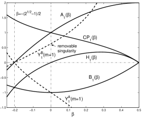
Figure 1: Variations of coefficients ${\cal A}_{1}(\beta)$, ${\cal B}_{1}(\beta)$, ${\cal C}{\cal P}_{1}(\beta)$, ${\cal H}_{1}(\beta)$ as defined in equation (36) and $D_{s}^{2}$ solutions of $Y_{1}^{A}|_{m=1}$ and $Y_{1}^{B}|_{m=1}$ with $\eta=1$ as obtained in equation (40) in the $\beta$ range of $\beta\in(-1/4,1/2)$.

$\beta$	$(-1/4,-(2^{1/2}-1)/2)$	$(-(2^{1/2}-1)/2,0)$	$(0,1/2)$
$C_{2}$	+	+	–
$1-{\cal C}{\cal P}_{1}$	–	–	+
${\cal A}_{1}(\beta)$	–	+	+
${\cal B}_{1}(\beta)$	–	–	–
${\cal H}_{1}(\beta)$	–	–	+
$Y_{1}^{A}|_{m=1}$	+	–	–
$Y_{1}^{B}|_{m=1}$	–	+	+
$\mu^{g}/\mu^{s}$	–	+	+

Table 1: Signs for various parameters when $\beta$ falls within the three contiguous subintervals of $\beta\in(-1/4,1/2)$ for the $m=1$ case. The phase relationship between $\mu^{g}$ and $\mu^{s}$ is only given for the physical solution branch with $D_{s}^{2}>0$ and remains valid for all combinations of $\delta$ and $\eta$. Specifically, $Y_{1}^{A}|_{m=1}$ is positive for $\beta\in(-1/4,\ -(2^{1/2}-1)/2)$, while $Y_{1}^{B}|_{m=1}$ is positive for $\beta\in(-(2^{1/2}-1)/2,\ 1/2)$.

3.1.1 The $m=1$ Aligned Case

The $m=1$ case is somewhat special corresponding to $1<{\cal C}{\cal P}_{1}<\pi^{4}/\{12[\Gamma(3/4)]^{8}\}\cong 1.596$ for $\beta\in(-1/4,\ 0)$ and to $0<{\cal C}{\cal P}_{1}<1$ for $\beta\in(0,\ 1/2)$, respectively. We know that for a composite system of coupled two SIDs with $\beta=0$ (i.e. flat rotation curves), the aligned $m=1$ case imposes no restriction on the dimensionless rotation parameter $D_{s}^{2}$ (Lou & Shen 2003). This situation changes qualitatively for $\beta\neq 0$. The additional freedom of $\beta$ parameter rules out that equation (38) be automatically satisfied for arbitrary $D_{s}^{2}$. We will see that to a certain extent, the aligned $m=1$ case is very similar to the spiral $m=1$ case in form. The dependence of solutions $y_{1}$ and $y_{2}$ on the square ratio of sound speeds $\eta$ and on the ratio of surface mass densities $\delta$ is distinctly different from those for the $m\geq 2$ cases. First we rewrite equations (40) and (41) for $m=1$ as

$$\begin{split}&Y_{1}^{A}|_{m=1}=\frac{{\cal A}_{1}}{{\cal B}_{1}}\ ,\quad\qquad\qquad Y_{1}^{B}|_{m=1}=\frac{(1-{\cal C}{\cal P}_{1}){\cal A}_{1}}{{\cal H}_{1}}\ ,\\ &Y_{\infty}^{A}|_{m=1}=-1+\frac{4\beta({\cal H}_{1}\delta+{\cal B}_{1})}{{\cal B}_{1}{\cal H}_{1}(1+\delta)}\ ,\qquad Y_{\infty}^{B}|_{m=1}=-1\ ,\end{split}$$

where except for a removable singularity at $\beta=0$ for $Y_{1}^{B}|_{m=1}$, the coefficients ${\cal A}_{1}$, ${\cal B}_{1}$, ${\cal C}{\cal P}_{1}$ and ${\cal H}_{1}$ as well as the $D_{s}^{2}$ solutions $Y_{1}^{A}$ and $Y_{1}^{B}$ as functions of $\beta$ are displayed in Fig. 1 within the open interval $\beta\in(-1/4,1/2)$. The sign variations of each parameters within the open interval $\beta\in(-1/4,1/2)$ are further summarized in Table 1 for reference.

For the $m=1$ case, the lower branch (either $y_{1}$ or $y_{2}$) of the solutions to equation (38) is always negative as can be seen later on and is therefore unphysical. It is possible for the upper branch of $D_{s}^{2}$ solution to be positive for a specific range of $\eta$, depending on the parameters $\beta$ and $\delta$ (see the critical $\eta_{c}$ discussed below). The variation within different parameter regimes is subtle for the special $m=1$ case as well as as for the phase relationship. And we only need to consider the positive portion in the upper branch of $D_{s}^{2}$ solution.

As indicated in Fig. 1 and Table 1, we divide the open interval of $-1/4<\beta<1/2$ into three subintervals to analyze properties of aligned coplanar perturbations with $m=1$.

1. for $-1/4<\beta<-(2^{1/2}-1)/2$ when $y_{1}>0$ is the upper branch

   As solutions $y_{1}$ and $y_{2}$ of equation (38) are both monotonic functions of $\eta$ (see the proof in Appendix B), we can use the explicit $y_{1}$ and $y_{2}$ solutions at $\eta=1$ [see solutions (40)] and $\eta\rightarrow\infty$ [see solutions (41)] to well bracket the ranges of $D_{s}^{2}$ value. For $\eta=1$, we have

   $$\begin{split}&y_{1}=Y_{1}^{A}|_{m=1}=\frac{{\cal A}_{1}}{{\cal B}_{1}}>0\ ,\\ &y_{2}=Y_{1}^{B}|_{m=1}=\frac{(1-{\cal C}{\cal P}_{1}){\cal A}_{1}}{{\cal H}_{1}}<0\ ,\end{split}$$ (43)

   while for $\eta\rightarrow\infty$, we have

   $$\begin{split}&y_{1}=Y_{\infty}^{A}|_{m=1}=-1+\frac{4\beta({\cal H}_{1}\delta+{\cal B}_{1})}{{\cal B}_{1}{\cal H}_{1}(1+\delta)}>-1\ ,\\ &y_{2}=Y_{\infty}^{B}|_{m=1}=-1\ .\end{split}$$ (44)

   In this case, the lower $y_{2}$ branch remains always negative and thus unphysical, while the upper $y_{1}$ branch increases monotonically with increasing $\delta$ and decreases monotonically with increasing $\eta$. For solutions (44), there exists a critical $\eta_{c}$ beyond which $y_{1}$ becomes negative for fixed values of $\beta$ and $\delta$. This $\eta_{c}$ can be explicitly determined by an analytical expression

   $$\begin{split}\eta_{c}=1+\frac{(1-{\cal C}{\cal P}_{1}){\cal A}_{1}(1+\delta)}{{\cal H}_{1}\delta+(1-{\cal C}{\cal P}_{1}){\cal B}_{1}}\ .\end{split}$$ (45)

   This expression (45) remains valid only when $\eta_{c}>1$ which further requires

   $$0<\delta<\frac{({\cal C}{\cal P}_{1}-1){\cal B}_{1}}{{\cal H}_{1}}<{\cal C}{\cal P}_{1}-1\ ,$$ (46)

   that in turn defines a critical value $\delta_{c}\equiv({\cal C}{\cal P}_{1}-1){\cal B}_{1}/{\cal H}_{1}$. For $\delta>\delta_{c}$, the upper $y_{1}$ branch remains always positive and physical.

   By equation (42), the phase relationship for surface mass density perturbations with $m=1$ corresponding to the physical portion of the $y_{1}$ branch is given by

   $$\frac{\mu^{g}}{\mu^{s}}=-1-\frac{{\cal B}_{1}(1+\delta)}{{\cal C}{\cal P}_{1}{\cal A}_{1}}+\frac{4\beta(1+\delta)}{{\cal C}{\cal P}_{1}{\cal A}_{1}(1+D_{s}^{2})}\ ,$$ (47)

   which decreases monotonically with increasing $D_{s}^{2}$ in the $\beta$ subinterval of case (I) and thus increases monotonically with increasing $\eta$ for the $y_{1}$ branch. We therefore have

   $$-1<\frac{\mu^{g}}{\mu^{s}}<\bigg{\{}\begin{array}[]{l l}(1+\delta-{\cal C}{\cal P}_{1})/({\cal C}{\cal P}_{1})<0,&\hbox{if $0<\delta<\delta_{c}$}\\ -{\cal C}{\cal P}_{1}{\cal A}_{1}\delta/({\cal H}_{1}\delta+{\cal B}_{1})<0,&\hbox{if $\delta>\delta_{c}$}\end{array}$$ (48)

   where the left-hand bound corresponds to $\eta=1$ and the right-hand bound corresponds either to $\eta=\eta_{c}$ when condition (46) is met or to $\eta\rightarrow\infty$ when $\delta>\delta_{c}$. At any rate, the phase relationship of surface mass density perturbations in the two coupled discs for the upper $y_{1}$ solution branch remains always out-of-phase.

   

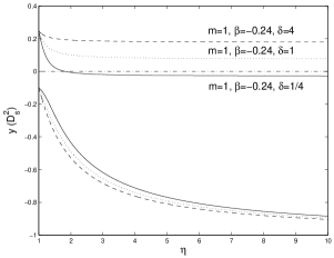
   (a) Case I: $-1/4<\beta<-(2^{1/2}-1)/2\ .$

   

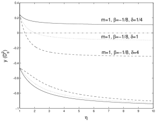
   (b) Case II: $-(2^{1/2}-1)/2<\beta<0\ .$

   

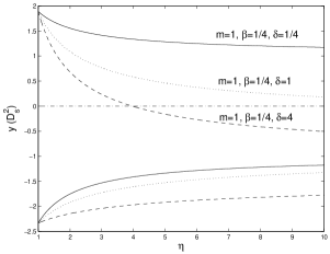
   (c) Case III: $0<\beta<1/2\ .$

   Figure 2: Two $D_{s}^{2}$ solution branches of equation (38) as functions of $\eta$ with combinations of $m=1$, $\beta=-0.24,\ -1/8,\ 1/4$ and $\delta=1/4,\ 1,\ 4$. For the same set of parameters in each panel (a), (b), (c), each linetype corresponds to two solutions of $D_{s}^{2}$ for a range of $1<\eta<10$.

2. for $-(2^{1/2}-1)/2<\beta<0$ when $y_{1}>0$ is the upper branch

   For $\eta=1$, we have

   $$\begin{split}&y_{1}=Y_{1}^{B}|_{m=1}=\frac{(1-{\cal C}{\cal P}_{1}){\cal A}_{1}}{{\cal H}_{1}}>0\ ,\\ &y_{2}=Y_{1}^{A}|_{m=1}=\frac{{\cal A}_{1}}{{\cal B}_{1}}<0\ ;\end{split}$$ (49)

   while for $\eta\rightarrow\infty$, we have

   $$\begin{split}&y_{1}=Y_{\infty}^{A}|_{m=1}=-1+\frac{4\beta({\cal H}_{1}\delta+{\cal B}_{1})}{{\cal B}_{1}{\cal H}_{1}(1+\delta)}>-1\ ,\\ &y_{2}=Y_{\infty}^{B}|_{m=1}=-1\ .\end{split}$$ (50)

   In this case again, the lower $y_{2}$ branch remains always negative and thus unphysical. The upper $y_{1}$ branch decreases monotonically with increasing either $\delta$ or $\eta$. The critical value of $\eta$ beyond which $y_{1}$ becomes negative for fixed values of $\beta$ and $\delta$ is again determined by the same expression (45). This criterion remains valid only when $\eta_{c}>1$ that further requires

   $$\delta>\delta_{c}\equiv\frac{({\cal C}{\cal P}_{1}-1){\cal B}_{1}}{{\cal H}_{1}}>{\cal C}{\cal P}_{1}-1\ .$$ (51)

   This then implies that for $0<\delta<\delta_{c}$, the upper $y_{1}$ branch of $D_{s}^{2}$ solution remains always physical for being positive.

   Similarly for the phase relationship between $\mu^{g}$ and $\mu^{s}$, we note that by expression (47), $\mu^{g}/\mu^{s}$ increases monotonically with increasing $D_{s}^{2}$ in the $\beta$ subinterval of case (II) and thus decreases monotonically with increasing $\eta$. We therefore have

   $$\delta>\frac{\mu^{g}}{\mu^{s}}>\bigg{\{}\begin{array}[]{l l}(1+\delta-{\cal C}{\cal P}_{1})/({\cal C}{\cal P}_{1})>0\ ,&\qquad\hbox{if $\delta>\delta_{c}$}\\ -{\cal C}{\cal P}_{1}{\cal A}_{1}\delta/({\cal H}_{1}\delta+{\cal B}_{1})>0\ ,&\hbox{if $0<\delta<\delta_{c}$}\end{array}$$ (52)

   where the left-hand bound corresponds to $\eta=1$ and the right-hand bound corresponds either to $\eta=\eta_{c}$ when condition (51) is satisfied or to $\eta\rightarrow\infty$ when $0<\delta<\delta_{c}$. At any rate, the phase relationship between $\mu^{g}$ and $\mu^{s}$ for the upper $y_{1}$ branch solution remains always in-phase with $\mu^{g}/\mu^{s}$ smaller than $\delta$.

3. for $0<\beta<1/2$ when $y_{2}$ becomes the upper branch

   For $\eta=1$, we have

   $$\begin{split}&y_{1}=Y_{1}^{A}|_{m=1}=\frac{{\cal A}_{1}}{{\cal B}_{1}}<0\ ,\\ &y_{2}=Y_{1}^{B}|_{m=1}=\frac{(1-{\cal C}{\cal P}_{1}){\cal A}_{1}}{{\cal H}_{1}}>0\ ;\end{split}$$ (53)

   while for $\eta\rightarrow\infty$, we have

   $$\begin{split}&y_{1}=Y_{\infty}^{A}|_{m=1}=-1+\frac{4\beta({\cal H}_{1}\delta+{\cal B}_{1})}{{\cal B}_{1}{\cal H}_{1}(1+\delta)}<-1,\\ &y_{2}=Y_{\infty}^{B}|_{m=1}=-1\ \qquad\qquad\qquad\hbox{if }\delta>-\frac{{\cal B}_{1}}{{\cal H}_{1}}\ ,\\ &\hbox{or else, }\\ &y_{1}=Y_{\infty}^{B}|_{m=1}=-1\ ,\\ &y_{2}=Y_{\infty}^{A}|_{m=1}=-1+\frac{4\beta({\cal H}_{1}\delta+{\cal B}_{1})}{{\cal B}_{1}{\cal H}_{1}(1+\delta)}>-1\\ &\hbox{if }0<\delta<-\frac{{\cal B}_{1}}{{\cal H}_{1}}\ .\end{split}$$ (54)

   In this case, the lower $y_{1}$ branch remains always negative and thus unphysical. The upper $y_{2}$ branch decreases monotonically with increasing either $\delta$ or $\eta$. The critical value of $\eta$ beyond which $y_{2}$ becomes negative for fixed values of $\beta$ and $\delta$ is also determined by expression (45). This criterion is valid only when $\eta_{c}>1$ which further requires

   $$\delta>\delta_{c}\equiv\frac{({\cal C}{\cal P}_{1}-1){\cal B}_{1}}{{\cal H}_{1}}\ ;$$ (55)

   this inequality in turn implies that for $0<\delta<\delta_{c}$ the upper $y_{2}$ branch remains always physical for being positive.

   Similarly by equation (47) for the phase relationship between $\mu^{g}$ and $\mu^{s}$, the ratio $\mu^{g}/\mu^{s}$ decreases monotonically with increasing $D_{s}^{2}$ in the $\beta$ subinterval of case (III) and thus increases monotonically with increasing $\eta$. We therefore have

   $$\delta<\frac{\mu^{g}}{\mu^{s}}<\bigg{\{}\begin{array}[]{l l}(1+\delta-{\cal C}{\cal P}_{1})/({\cal C}{\cal P}_{1})>0\ ,&\hbox{if $\delta>\delta_{c}$}\\ -({\cal C}{\cal P}_{1}{\cal A}_{1}\delta)/({\cal H}_{1}\delta+{\cal B}_{1})>0\ ,&\hbox{if $0<\delta<\delta_{c}$}\end{array}$$ (56)

   where the left-hand bound corresponds to $\eta=1$ and the right-hand bound corresponds either to $\eta=\eta_{c}$ when condition (55) is satisfied or to $\eta\rightarrow\infty$ when $0<\delta<\delta_{c}$. At any rate, the phase relationship between $\mu^{g}$ and $\mu^{s}$ for the upper $y_{2}$ branch solution remains always in-phase with $\mu^{g}/\mu^{s}$ greater than $\delta$.

Relevant details of illustrating examples for three cases of $\beta=-0.24$, $\beta=-1/8$ and $\beta=1/4$ respectively are shown in three panels (a), (b) and (c) of Fig. 2 and are also summarized in Table 2.

		$\beta=-0.24$		$\beta=-1/8$		$\beta=1/4$
$m$	$\delta$	$\delta_{c}$	$\eta_{c}$	$\delta_{c}$	$\eta_{c}$	$\delta_{c}$	$\eta_{c}$
1	1/4	0.401	1.821	0.522	/	0.809	/
	1	0.401	/	0.522	2.018	0.809	20.812
	4	0.401	/	0.522	1.350	0.809	3.959
2	1/4	/	2.514	/	2.375	/	2.033
	1		1.813		1.803		1.809
	4		1.556		1.567		1.664
3	1/4		2.641		2.278		1.782
	1		2.147		1.947		1.681
	4		1.881		1.752		1.604

Table 2: The critical values of $\eta_{c}$ and $\delta_{c}$ for the three cases of $\beta=-0.24$, $-1/8$ and $1/4$ with different values of $m=1,2,3$ and $\delta$. A slash “/” means that the critical $\eta_{c}$ or $\delta_{c}$ do not exist. Note that only for the $m=1$ case does there exist such a critical $\delta_{c}$ that depends only on $\beta$.

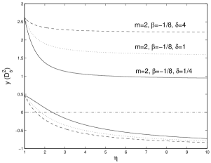
(a) $m=2,\ \beta=-1/8,\ \delta=4,\ 1,\ 1/4$

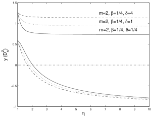
(b) $m=2,\ \beta=1/4,\ \delta=4,\ 1,\ 1/4$

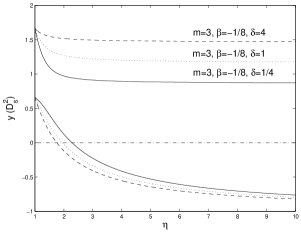
(c) $m=3,\ \beta=-1/8,\ \delta=4,\ 1,\ 1/4$

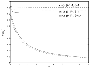
(d) $m=3,\ \beta=1/4,\ \delta=4,\ 1,\ 1/4$

Figure 3: Aligned $D_{s}^{2}$ solution curves $y_{1}$ and $y_{2}$ as functions of $\eta$ for different azimuthal periodicities $m=2,3$ and surface mass density ratio $\delta=1/4,1,4$ with two fixed values of $\beta=-1/8$ and $\beta=1/4$. For the same set of parameters in each panel (a), (b), (c), (d), each linetype corresponds to two solutions of $D_{s}^{2}$ for a range of $1<\eta<10$.

3.1.2 The $m\geq 2$ Aligned Cases

When $m\geq 2$, we have $C_{2}>0$, $0<{\cal C}{\cal P}_{m}<1$, ${\cal A}_{m}>0$, ${\cal B}_{m}>0$, ${\cal H}_{m}>0$ in the open $\beta$ interval $\beta\in(-1/4,1/2)$. Therefore in this case of $m\geq 2$, $y_{1}$ and $y_{2}$ remain always upper and lower branches, respectively. By solutions (40) for $\eta=1$, we have

$$\begin{split}&y_{1}=Y_{1}^{A}=\frac{{\cal A}_{m}}{{\cal B}_{m}}>0\ ,\\ &y_{2}=Y_{1}^{B}=\frac{(1-{\cal C}{\cal P}_{m}){\cal A}_{m}}{{\cal H}_{m}}>0\ ,\\ \end{split}$$ (57)

while by solutions (41) for $\eta\rightarrow\infty$, we have

$$\begin{split}&y_{1}=Y_{\infty}^{A}=\frac{{\cal A}_{m}[{\cal H}_{m}\delta+(1-{\cal C}{\cal P}_{m}){\cal B}_{m}]}{{\cal B}_{m}{\cal H}_{m}(1+\delta)}>0\ ,\\ &y_{2}=Y_{\infty}^{B}=-1\ .\end{split}$$ (58)

As the limiting situations for $\eta=1$ and $\eta\rightarrow\infty$ well bracket possible ranges of $y_{1}$ and $y_{2}$ branches (see Appendix B), it is obvious that the upper $y_{1}$ branch remains always positive and the value of $y_{1}$ increases with increasing $\delta$ and decreases with increasing either $m$ or $\eta$. Meanwhile, the lower $y_{2}$ branch has a specific critical value $\eta_{c}$ of $\eta$ beyond which the $y_{2}$ solution becomes unphysical for being negative. This critical value $\eta_{c}$ is given by

$$\eta_{c}=1+\frac{(1-{\cal C}{\cal P}_{m}){\cal A}_{m}(1+\delta)}{{\cal H}_{m}\delta+(1-{\cal C}{\cal P}_{m}){\cal B}_{m}}\ ,$$ (59)

where we have ${\cal H}_{m}$ always greater than $m$ for all $m\geq 2$ within $\beta\in(-1/4,1/2)$. Such a critical $\eta_{c}$ always exists for the $y_{2}$ branch for all values of $\delta$. In other words, there does not exist a critical value $\delta_{c}$ for $\delta$ as in the aligned $m=1$ case.

This critical value $\eta_{c}$ of $\eta$ decreases with increasing $\delta$, much like the case of two coupled SIDs investigated recently (Lou & Shen 2003). For physical regimes of $y_{1}$ and $y_{2}$, they both decrease monotonically with increasing $\eta$, while $y_{1}$ branch increases monotonically and $y_{2}$ branch decreases monotonically with increasing $\delta$.

For the phase relationship between $\mu^{g}$ and $\mu^{s}$, it is straightforward to show that the ratio $\mu^{g}/\mu^{s}$ decreases monotonically with increasing $D_{s}^{2}$ and thus increases monotonically with increasing $\eta$ for $m\geq 2$. For the upper $y_{1}$ branch, we obtain

$$\begin{split}-1&<\frac{\mu^{g}}{\mu^{s}}<-\frac{{\cal C}{\cal P}_{m}{\cal A}_{m}\delta}{{\cal H}_{m}\delta+{\cal B}_{m}}\ ,\end{split}$$ (60)

where the left-hand bound corresponds to $\eta=1$ and the right-hand bound corresponds to $\eta\rightarrow\infty$. In the specified range of $\beta\in(-1/4,1/2)$, the ratio $\mu^{g}/\mu^{s}$ remains always negative for the upper $y_{1}$ branch, indicating surface mass density perturbations in two discs are out-of-phase.

For the lower $y_{2}$ branch in parallel, we derive

$$\delta<\frac{\mu^{g}}{\mu^{s}}<\frac{1+\delta}{{\cal C}{\cal P}_{m}}-1\ ,$$ (61)

where the left-hand bound corresponds to $\eta=1$ and the right-hand bound corresponds to the critical $\eta_{c}$ which makes $D_{s}^{2}=y_{2}=0$. Apparently, the lower $y_{2}$ branch (if physical) means surface mass density perturbations in the two coupled discs are in-phase.

3.2 Spiral Coplanar Perturbation Configurations

Stationary surface mass density perturbations in both discs scale in the forms of $\propto\mu e^{-\hbox{i}m\theta}$ in azimuthal angle $\theta$. For aligned perturbations, we have further taken $\mu\propto r^{-\varepsilon}$ where $\varepsilon$ is a positive/negative constant exponent. For example in subsection 3.1, we have chosen $\varepsilon=\alpha=1+2\beta$ for coplanar perturbations carrying the same radial power-law dependence of the background equilibrium disc system. On the other hand, for $\varepsilon$ being a complex constant exponent, perturbations would appear in spiral forms, namely, the so-called logarithmic spiral $\mu\propto r^{-\Re(\varepsilon)}\exp[-\hbox{i}\Im(\varepsilon)\ln r]$ where $\Re(\varepsilon)$ and $\Im(\varepsilon)$ are the real and imaginary parts of $\varepsilon$. To ensure the gravitational potential perturbation arising from this perturbed surface mass density as computed by Poisson integral (4) being finite requires $-m+1<\Re(\varepsilon)<m+2$ (Qian 1992). Without loss of generality, we assume a set of logarithmic spiral density perturbations and the resulting gravitational potential perturbation in a mathematically consistent manner (Kalnajs 1971; Syer & Tremaine; Shu et al. 2000; Lou 2002; Lou & Fan 2002; Lou & Shen 2003; Lou & Zou 2004; Lou & Wu 2004). Specifically, we write

$$\begin{split}&\mu^{s}=\sigma^{s}r^{-3/2}\exp(\hbox{i}\xi\ln r)\ ,\qquad\mu^{g}=\sigma^{g}r^{-3/2}\exp(\hbox{i}\xi\ln r)\ ,\\ &V=-2\pi Gr(\mu^{s}+\mu^{g}){\cal N}_{m}(\xi)\ ,\end{split}$$ (62)

where $\sigma^{s}$ and $\sigma^{g}$ are small constant coefficients,

$${\cal N}_{m}(\xi)=\frac{\Gamma(m/2+\hbox{i}\xi/2+1/4)\Gamma(m/2-\hbox{i}\xi/2+1/4)}{2\Gamma(m/2+\hbox{i}\xi/2+3/4)\Gamma(m/2-\hbox{i}\xi/2+3/4)}$$ (63)

is the Kalnajs function (Kalnajs 1971) and $\xi$ is a kind of radial ‘wavenumber’. We refresh a few properties of ${\cal N}_{m}(\xi)$. First, ${\cal N}_{m}(\xi)$ is an even function of $\xi$ so only $\xi\geq 0$ will be considered later. Secondly, ${\cal N}_{m}(\xi)$ decreases monotonically with increasing $\xi>0$. Thirdly, $0<{\cal N}_{m}<1$ for $m\geq 1$ while ${\cal N}_{0}$ is positive and can be greater than 1 for a sufficiently small $\xi$.

The choice of such form of perturbations is different from that of Syer & Tremaine (1996), whose spiral perturbations were taken to be $\mu\propto r^{-1-2\beta}\exp(\hbox{i}m\xi\ln r)$ for $m>0$ (analysis before subsection 3.4 in their paper) in our notations. For axisymmetric stability analysis in their subsection 3.4, they adopted the same spiral perturbations in the form of (62) (see also Lemos et al. 1991). We note that our background equilibria as well as the adopted form of logarithmic spiral perturbations are themselves scale-free, separately, whereas combinations of the background equilibrium and perturbations are not scale-free except for the special $\beta=1/4$ case (see Lynden-Bell & Lemos 1993).

Parallelling with ${\cal P}_{m}$ for the case of aligned perturbations, there are two useful formulae for ${\cal N}_{m}(\xi)$ for logarithmic spiral perturbations. The first one is the recursion relation

$${\cal N}_{m+1}(\xi){\cal N}_{m}(\xi)=[(m+1/2)^{2}+\xi^{2}]^{-1}\ ,$$ (64)

and the second one is the asymptotic expression for ${\cal N}_{m}(\xi)$

$${\cal N}_{m}(\xi)\approx(m^{2}+\xi^{2}+1/4)^{-1/2}$$ (65)

for $m^{2}+\xi^{2}\gg 1$. For $m\geq 2$, this asymptotic expression (65) is accurate enough to compute values of ${\cal N}_{m}(\xi)$.

Using potential-density set of (62) for logarithmic spirals, we rearrange stationary coplanar perturbation equations (27) and (28) into the following forms with $m>0$.

$$\begin{split}&\mu^{s}=\bigg{(}\frac{m^{2}+2\beta}{r}-2\frac{d}{dr}-r\frac{d^{2}}{dr^{2}}\bigg{)}(H_{1}r\mu^{s}+G_{1}r\mu^{g})\ ,\\ &\mu^{g}=\bigg{(}\frac{m^{2}+2\beta}{r}-2\frac{d}{dr}-r\frac{d^{2}}{dr^{2}}\bigg{)}(H_{2}r\mu^{g}+G_{2}r\mu^{s})\ ,\\ \end{split}$$ (66)

where the four relevant coefficients $H_{1}$, $H_{2}$, $G_{1}$ and $G_{2}$ are defined here explicitly by

$$\begin{split}&H_{1}\equiv\frac{1}{D_{s}^{2}(1+2\beta)(m^{2}-2+2\beta)}\\ &\qquad\qquad\qquad\times\bigg{[}1-\frac{(1+2\beta)(1+D_{s}^{2})}{2\beta{\cal P}_{0}}\frac{{\cal N}_{m}}{(1+\delta)}\bigg{]}\ ,\\ &H_{2}\equiv\frac{1}{D_{g}^{2}(1+2\beta)(m^{2}-2+2\beta)}\\ &\qquad\qquad\qquad\times\bigg{[}1-\frac{(1+2\beta)(1+D_{g}^{2})}{2\beta{\cal P}_{0}}\frac{{\cal N}_{m}\delta}{(1+\delta)}\bigg{]}\ ,\\ &G_{1}\equiv-\frac{(1+D_{s}^{2})}{D_{s}^{2}(2\beta{\cal P}_{0})(m^{2}-2+2\beta)}\frac{{\cal N}_{m}}{(1+\delta)}\ ,\\ &G_{2}\equiv-\frac{(1+D_{g}^{2})}{D_{g}^{2}(2\beta{\cal P}_{0})(m^{2}-2+2\beta)}\frac{{\cal N}_{m}\delta}{(1+\delta)}\ .\\ \end{split}$$ (67)

Rewriting equations (66) with expressions (62) for $\mu^{s}$ and $\mu^{g}$, we immediately obtain

$$\begin{split}&[1-H_{1}(m^{2}+\xi^{2}+1/4+2\beta)]\mu^{s}\\ &\qquad\qquad\qquad\qquad=G_{1}(m^{2}+\xi^{2}+1/4+2\beta)\mu^{g}\ ,\\ &[1-H_{2}(m^{2}+\xi^{2}+1/4+2\beta)]\mu^{g}\\ &\qquad\qquad\qquad\qquad=G_{2}(m^{2}+\xi^{2}+1/4+2\beta)\mu^{s}\ .\end{split}$$ (68)

As for the aligned case in subsection 3.1, we define some useful notations for parameter combinations that will simplify our following derivations, namely

$$\begin{split}&{\cal A}_{m}(\beta,\xi)\equiv m^{2}+\xi^{2}+1/4+2\beta\ ,\\ &{\cal B}_{m}(\beta)\equiv(1+2\beta)(m^{2}-2+2\beta)\ ,\\ &{\cal C}(\beta)\equiv(1+2\beta)/(2\beta{\cal P}_{0})\ ,\\ &{\cal H}_{m}(\beta,\xi)\equiv{\cal C}{\cal N}_{m}{\cal A}_{m}+{\cal B}_{m}\ .\end{split}$$ (69)

With convenient notations (69), equation (68) leads to the following stationary dispersion relation

$$(1-H_{1}{\cal A}_{m})(1-H_{2}{\cal A}_{m})=G_{1}G_{2}{\cal A}_{m}^{2}$$ (70)

for coplanar logarithmic spiral perturbations in a composite disc system.

Substituting expressions (67) of $H_{1}$, $H_{2}$, $G_{1}$ and $G_{2}$ into stationary dispersion relation (70) and using the background condition $D_{g}^{2}=\eta(D_{s}^{2}+1)-1$, we obtain one quadratic equation in terms of $y\equiv D_{s}^{2}$, namely

$$C_{2}y^{2}+C_{1}y+C_{0}=0\ ,$$ (71)

where coefficients $C_{2}$, $C_{1}$ and $C_{0}$ are functions of parameters $m$, $\beta$, $\delta$, $\eta$ and $\xi$, and are defined by

$$\begin{split}C_{2}=&{\cal B}_{m}{\cal H}_{m}\eta\ ,\\ C_{1}=&\bigg{[}({\cal B}_{m}-{\cal A}_{m}){\cal H}_{m}+\frac{({\cal A}_{m}+{\cal B}_{m})({\cal H}_{m}-{\cal B}_{m})}{(1+\delta)}\bigg{]}\eta\\ &\qquad\qquad\qquad-\frac{({\cal A}_{m}+{\cal B}_{m})({\cal H}_{m}+{\cal B}_{m}\delta)}{(1+\delta)}\ ,\\ C_{0}=&\bigg{[}-{\cal A}_{m}{\cal H}_{m}+\frac{({\cal A}_{m}+{\cal B}_{m})({\cal H}_{m}-{\cal B}_{m})}{(1+\delta)}\bigg{]}\eta\\ &\qquad+({\cal A}_{m}+{\cal B}_{m})^{2}-\frac{({\cal A}_{m}+{\cal B}_{m})({\cal H}_{m}+{\cal B}_{m}\delta)}{(1+\delta)}\ .\end{split}$$ (72)

Given specific values for $m$, $\beta$, $\delta$ and $\eta$, we readily solve quadratic equation (71) analytically for each ‘radial wavenumber’ $\xi$ for stationary logarithmic spirals. Again for a non-negative determinant as proven in Appendix A, there are two real $D_{s}^{2}$ solutions to equation (71), namely

$$y_{1,2}=\frac{-C_{1}\pm(C_{1}^{2}-4C_{2}C_{0})^{1/2}}{2C_{2}}\ .$$

In addition to the well-studied isothermal $\beta=0$ case (Lou & Shen 2003; Lou & Zou 2004), we follow a similar procedure of analyzing the aligned case to construct logarithmic spiral configurations for the composite disc system in the range of $\beta\in(-1/4,1/2)$. For astrophysical relevance, we specifically choose $\beta=-1/8$ and $\beta=1/4$ as illustrating examples. Values of $\delta$ are chosen as 1/4, 1 and 4 with $\eta>1$. For $\eta=1$, coefficients $C_{2}$, $C_{1}$ and $C_{0}$ as defined by expressions (72) are again independent of $\delta$.

We now derive $y=D_{s}^{2}$ solutions below for the cases of $\eta=1$ and $\eta\rightarrow\infty$ separately for the same rationale as explained in the analysis of the aligned case. In terms of coefficients (69), the two explicit $D_{s}^{2}$ solutions to stationary dispersion relation (71) when $\eta=1$ are

$$Y_{1}^{A}=\frac{{\cal A}_{m}}{{\cal B}_{m}}\ \ \qquad\hbox{ and }\qquad Y_{1}^{B}=\frac{(1-{\cal C}{\cal N}_{m}){\cal A}_{m}}{{\cal H}_{m}}\ .$$ (73)

Since the ratio of sound speeds in the two discs are the same for $\eta=1$, the composite system of two coupled discs may be treated as one single disc to a certain extent. In fact, the second expression $Y_{1}^{B}$ in equation (73) is simply the result for the case of a single disc, while the first expression $Y_{1}^{A}$ in equation (73) is additional due to the gravitational coupling between the two discs. Under some circumstances (e.g., $m=0\hbox{ and }1$) when $Y_{1}^{A}$ remains always negative, we may practically regard the two-disc system as being identical with the case of a single disc for $\eta=1$.

The two explicit $D_{s}^{2}$ solutions to stationary dispersion relation (71) in the limit of $\eta\rightarrow\infty$ are

$$Y_{\infty}^{A}=\frac{{\cal A}_{m}[{\cal H}_{m}\delta+(1-{\cal C}{\cal N}_{m}){\cal B}_{m}]}{{\cal B}_{m}{\cal H}_{m}(1+\delta)}\ \ \quad\hbox{and}\quad\ Y_{\infty}^{B}=-1\ .$$ (74)

Meanwhile, the phase relationship for surface mass density perturbations reads from (68) as

$$\frac{\mu^{g}}{\mu^{s}}=\frac{1-H_{1}{\cal A}_{m}}{G_{1}{\cal A}_{m}}=-1-\frac{(D_{s}^{2}{\cal B}_{m}-{\cal A}_{m})(1+\delta)}{{\cal N}_{m}{\cal A}_{m}(1+D_{s}^{2})}\ .$$ (75)

As expected, all the expressions for the logarithmic spiral case can be obtained from those for the aligned case by simply replacing ${\cal P}_{m}$ with ${\cal N}_{m}$ resulting from different potential-density pairs. This comes naturally from the perspective that both aligned and spiral configurations are coplanar density waves propagating relative to the discs in either purely azimuthal directions or both radial and azimuthal directions (Lou 2002; Lou & Shen 2003).

3.2.1 Marginal Stability of Axisymmetric Disturbances

It is reminded that for the aligned case, axisymmetric $m=0$ perturbations merely represent a rescaling of the background equilibrium state of axisymmetry. For the $m=0$ case with radial oscillations, we should not start from equations (27) and (28), but instead should use equation (2.3) by first setting $m=0$ with $\omega\neq 0$ and then take the limit of $\omega\rightarrow 0$. It is then straightforward to obtain

$$\begin{split}&[1-H_{1}(\xi^{2}+1/4)]\mu^{s}=G_{1}(\xi^{2}+1/4)\mu^{g}\ ,\\ &[1-H_{2}(\xi^{2}+1/4)]\mu^{g}=G_{2}(\xi^{2}+1/4)\mu^{s}\ ,\end{split}$$ (76)

where coefficients $H_{1}$, $H_{2}$, $G_{1}$ and $G_{2}$ are evaluated by simply setting $m=0$ in definitions (67). It is clear that equation (76) for the $m=0$ case with radial oscillations differs from equation (68) for non-axisymmetric spiral cases. In definitions (69), we only need to replace ${\cal A}_{0}$ by ${\cal A^{\prime}}_{0}=\xi^{2}+1/4$ and redefine ${\cal H}_{0}={\cal C}{\cal N}_{0}{\cal A^{\prime}}_{0}+{\cal B}_{0}$, and then use the explicit solutions derived for $m>0$ spiral cases in Section 3.2 by setting $m=0$. The marginal stability curves thus obtained are displayed in Fig. 4$-$9. We show the complete $y\equiv D_{s}^{2}$ solution structure versus $\xi$ while only the portions above $y=0$ are physically sensible.

To analyze the solution properties as parameters $\beta$, $\delta$, $\eta$ and ‘radial wavenumber’ $\xi$ vary for the axisymmetric $m=0$ case, we use asymptotic expression (65) for ${\cal N}_{4}(\xi)$ and then use recursion relation (64) to derive an approximate analytical expression to compute the value of ${\cal N}_{0}(\xi)$, namely

$$\begin{split}{\cal N}_{0}(\xi)&=\frac{1}{2}\frac{\Gamma(1/4+\hbox{i}\xi/2)\Gamma(1/4-\hbox{i}\xi/2)}{\Gamma(3/4+\hbox{i}\xi/2)\Gamma(3/4-\hbox{i}\xi/2)}\\ &\approx\frac{(9/4+\xi^{2})(49/4+\xi^{2})}{(1/4+\xi^{2})(25/4+\xi^{2})(65/4+\xi^{2})^{1/2}}\ \end{split}$$ (77)

with relative errors less than $0.5\%$.

In the $\beta$ interval of $\beta\in(-1/4,1/2)$, the quadratic coefficient $C_{2}$ of stationary dispersion relation (71) vanishes when

$${\cal H}_{0}={\cal C}{\cal N}_{0}{\cal A^{\prime}}_{0}+{\cal B}_{0}=0\ ,$$ (78)

which for a specified $\beta$ determines the value of $\xi=\xi_{c}$ at which the value of $D_{s}^{2}$ will approach infinity. It is found that in the open interval of $\beta\in(-1/4,1/2)$, there exists only one such $\xi_{c}$ where ${\cal H}_{0}$ vanishes as can be numerically computed. Moreover for $0<\xi<\xi_{c}$, we have ${\cal H}_{0}<0$ so that $C_{2}>0$, while for $\xi>\xi_{c}$, we have ${\cal H}_{0}>0$ so that $C_{2}<0$. This means that for wavenumber $\xi<\xi_{c}$, the upper branch is always $y_{1}$, while for wavenumber $\xi>\xi_{c}$, the upper branch is always $y_{2}$.

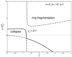
Figure 4: Two branches of solutions to equation (71) for $m=0$, $\beta=-1/8$ and $\eta=1$. The divergent point is $\xi_{c}=1.217$. In this case of $\eta=1$, the value of $\delta$ can be arbitrary. The $y_{1}$ branch is plotted in heavy solid line segments and the $y_{2}$ branch is plotted in heavy dashed line segments.

First, we closely examine the $\beta=-1/8$ case. This critical $\xi_{c}$ is numerically determined from equation (78) as $\xi_{c}=1.217$. We choose $\eta=1$ as a limiting case and the two explicit $D_{s}^{2}$ solutions from equation (73) are

$$\begin{split}&Y_{1}^{A}=\frac{{\cal A^{\prime}}_{0}}{{\cal B}_{0}}=-\frac{16}{27}\xi^{2}-\frac{4}{27}\ ,\\ &Y_{1}^{B}=\frac{(1-{\cal C}{\cal N}_{0}){\cal A^{\prime}}_{0}}{{\cal H}_{0}}=\frac{(1-{\cal C}{\cal N}_{0})(\xi^{2}+1/4)}{{\cal C}{\cal N}_{0}(\xi^{2}+1/4)-27/16}\ .\end{split}$$ (79)

We stress here that $Y_{1}^{A}$ and $Y_{1}^{B}$ do not correspond to $y_{1}$ and $y_{2}$ solutions, respectively, in a simple manner, because signs of coefficients vary with $\xi$. For instance in Fig. 4, we display $y_{1}$ in solid line and $y_{2}$ in dashed line. Across $\xi_{c}$, solution structures changes abruptly. For physically reasonable marginal stability curves, we only need the portions above $y=0$. The two unstable regimes shown in Fig. 4 are the ring fragmentation regime where a composite disc system rotates too fast to be stable and the collapse regime where a composite disc system rotates too slowly to be stable against large-scale Jeans collapse (Lemos et al. 1991; Syer & Tremaine 1996; Shu et al. 2000; Lou 2002; Lou & Fan 2002; Lou & Shen 2003; Lou & Zou 2004). These marginal stability curves can also be derived from the time-dependent WKBJ analysis by imposing the scale-free disc conditions (Shen & Lou 2003), with the more straightforward $D_{s}-$criterion equivalent to the effective $Q$ parameters presented by Elmegreen (1995) and Jog (1996). By varying the sound speed ratio $\eta$ and disc density ratio $\delta$, we obtain similar marginal stability curves in Fig. 5. The trends are qualitatively the same as the isothermal $\beta=0$ case (Lou & Shen 2003; Shen & Lou 2003). In other words, a composite disc system is less stable as compared with a single disc system for overall axisymmetric instabilities but becomes more difficult for large-scale collapses (Lou & Shen 2003; Shen & Lou 2003).

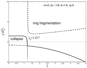
(a) $m=0$, $\beta=-1/8$, $\delta=1/4$, $\eta=5$

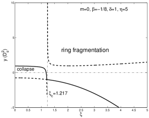
(b) $m=0$, $\beta=-1/8$, $\delta=1$, $\eta=5$

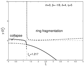
(c) $m=0$, $\beta=-1/8$, $\delta=4$, $\eta=5$

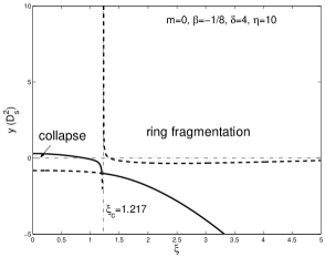
(d) $m=0$, $\beta=-1/8$, $\delta=4$, $\eta=10$

Figure 5: Two $D_{s}^{2}$ solution branches of stationary dispersion relation (71) with radial oscillations for $m=0$, $\beta=-1/8$, $\eta=5,\ 10$ and $\delta=1/4,\ 1,\ 4$. In each panel (a), (b), (c), (d), the segments above $y=0$ constitute the marginal stability curves as indicated.

Next, we consider the case of $\beta=1/4$. The divergent point now becomes $\xi_{c}=3.159$. For qualitative results, we again start from the special case of $\eta=1$ with the two $D_{s}^{2}$ solutions of stationary dispersion relation (71) explicitly given by

$$\begin{split}&Y_{1}^{A}=\frac{{\cal A^{\prime}}_{0}}{{\cal B}_{0}}=-4\xi^{2}/9-1/9\ ,\\ &Y_{1}^{B}=\frac{(1-{\cal C}{\cal N}_{0}){\cal A^{\prime}}_{0}}{{\cal H}_{0}}=\frac{(1-{\cal C}{\cal N}_{0})(\xi^{2}+1/4)}{{\cal C}{\cal N}_{0}(\xi^{2}+1/4)-9/4}\ .\end{split}$$ (80)

The corresponding marginal stability curves are displayed in Fig. 6. We further explored variations of the marginal stability curves for different sets of parameters in Fig. 7.

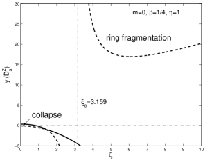
Figure 6: Two branches of $D_{s}^{2}$ solutions to stationary dispersion relation (71) with radial oscillations for $m=0$, $\beta=1/4$ and $\eta=1$. The divergent point is at $\xi_{c}=3.159$. In this case of $\eta=1$, $\delta$ can be arbitrary.

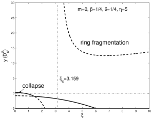
(a) $m=0$, $\beta=1/4$, $\delta=1/4$, $\eta=5$

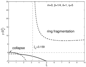
(b) $m=0$, $\beta=1/4$, $\delta=1$, $\eta=5$

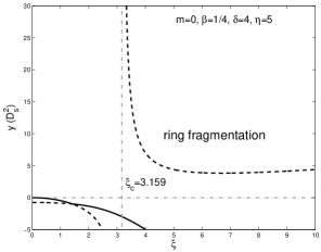
(c) $m=0$, $\beta=1/4$, $\delta=4$, $\eta=5$

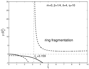
(d) $m=0$, $\beta=1/4$, $\delta=4$, $\eta=10$

Figure 7: Two $D_{s}^{2}$ solution branches of stationary dispersion relation (71) with radial oscillations for $m=0$, $\beta=1/4$, $\eta=5,\ 10$ and $\delta=1/4,\ 1,\ 4$. In each panel (a), (b), (c), (d), the curve segments above $y=0$ constitute the marginal stability curves as indicated.

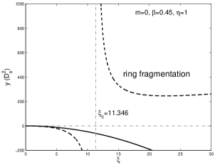
Figure 8: Two $D_{s}^{2}$ solution branches to stationary dispersion relation (71) with radial oscillations for $m=0$, $\beta=0.45$ and $\eta=1$. The divergent point is at $\xi_{c}=11.346$. In this case of $\eta=1$, the value of $\delta$ can be arbitrary.

There exists a critical $\beta_{c}$ above which the collapse regime disappears even for the $\eta=1$ (single disc) case when the collapse region is largest. This critical $\beta_{c}=0.436$ is determined by the condition of zero collapsed regime for the maximum of the lower-left branch, namely

$$Y_{1}^{B}=\frac{(1-{\cal C}{\cal N}_{0}){\cal A^{\prime}}_{0}}{{\cal H}_{0}}\bigg{|}_{\xi=0}=0\ .$$ (81)

In order to see this clearly, we take $\beta=0.45$ and obtain marginal stability curves for $\eta=1$ as shown in Fig. 8 where no collapse regime appears. This result is consistent with that of Syer & Tremaine (1996) as can be seen from their fig. 2 for the marginal axisymmetric stable curve in terms of their $w=1/[(1+2\beta)D_{s}^{2}]$ as noted earlier near the end of subsection 2.2 for notational correspondences.

With the analysis technique developed by Shen & Lou (2003), we can perform time-dependent WKBJ analysis for a composite system of two coupled scale-free discs described in Section 2. For the above three cases with $\beta=-1/8$, $1/4$ and $0.45$, we display contours of frequency $\omega^{2}$ in terms of the effective radial wavenumber $\xi\equiv K\equiv|k|r$ and the rotation parameter $D_{s}^{2}$ in the same figure of exact stationary perturbation configurations in Fig. 9 for the $\eta=1$ case corresponding to the single disc case. The zero-frequency lines (i.e., marginal stability curves) for both precise and WKBJ approximation accord well with each other for large radial wavenumber when the WKBJ approximation is valid; for small radial wavenumber, the WKBJ approximation breaks down and the two regimes differ significantly as expected.

In this context, we note the axisymmetric stability analysis by Lemos et al. (1991) in a single-disc system. Lemos et al. (1991) derived the same axisymmetric background equilibrium state for a single disc. For perturbations, they imposed adiabatic approximation with the adiabatic index $\gamma$ greater than 1 and independent of the barotropic index $n$ used for the equilibrium state, which is different from Syer & Tremaine (1996) and our present analysis.

In the global analysis on axisymmetric $m=0$ instabilities with radial oscillations, stationary $\omega=0$ wave patterns mark the onset of instabilities (Lemos et al. 1991; Syer & Tremaine 1996; Lou 2002; Lou & Fan 2002; Shu et al. 2000; Lou & Shen 2003; Shen & Lou 2003; Lou & Zou 2004) in a composite disc system. Apparently, there are two unstable regimes, namely, the long wavelength collapse regime and the short wavelength ring fragmentation regime. Therefore, the stability criterion for $D_{s}^{2}$ falls in a range whose width increases with increasing $\beta$. Both regimes of the collapse instability and the ring fragmentation instability are reduced for larger values of $\beta$. As already noted, for $\beta>0.436$, the collapse regime disappears completely. For sufficiently small values of $\beta<-0.130$, the stable range of $D_{s}^{2}$ does not exist (see Appendix D for details). As remarked earlier, a composite system of two coupled discs is less stable than a single disc system. The introduction of an additional gaseous disc with larger $\delta$ and $\eta$ will reduce the overall stable range of $D_{s}^{2}$, while tending to suppress the regime of collapse for large-scale instabilities (Lou & Shen 2003; Lou & Zou 2004).

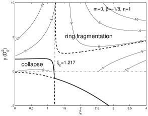
(a) $m=0$, $\beta=-1/8$, $\eta=1$

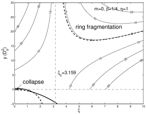
(b) $m=0$, $\beta=1/4$, $\eta=1$

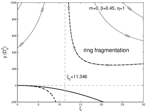
(c) $m=0$, $\beta=0.45$, $\eta=1$

Figure 9: A comparison of stability boundary for exact global stationary perturbation configurations obtained here for $m=0$ with radial oscillations and of the zero-frequency boundary in the WKBJ analysis (Shen & Lou 2003) for three cases: $\beta=-1/8$, $1/4$ and $0.45$ with $\eta=1$.

3.2.2 The Logarithmic Spiral $m=1$ Case

The logarithmic spiral $m=1$ case behaves qualitatively different from the aligned $m=1$ case. The reason is simply that the additional radial wavenumber parameter $\xi$ will also alter values of coefficients in equation (71).

In this case, we again use asymptotic expression (65) to estimate ${\cal N}_{4}(\xi)$ and then use recursion relation (64) to derive an approximate analytical expression for ${\cal N}_{1}(\xi)$, namely

$$\begin{split}{\cal N}_{1}&=\frac{1}{2}\frac{\Gamma(3/4+\hbox{i}\xi/2)\Gamma(3/4-\hbox{i}\xi/2)}{\Gamma(5/4+\hbox{i}\xi/2)\Gamma(5/4-\hbox{i}\xi/2)}\\ &\approx\frac{(25/4+\xi^{2})(65/4+\xi^{2})^{1/2}}{(9/4+\xi^{2})(49/4+\xi^{2})}\ \end{split}$$ (82)

with relative error less than $0.5\%$. With ${\cal A}_{1}=\xi^{2}+5/4+2\beta$ and ${\cal B}_{1}=4\beta^{2}-1$ according to definitions (69), we immediately obtain

$${\cal H}_{1}={\cal C}{\cal N}_{1}(\xi^{2}+5/4+2\beta)+4\beta^{2}-1\ ,$$ (83)

which increases monotonically with increasing $\xi$ for fixed $\beta$ values and attains its minimum value at $\xi=0$ as

$${\cal H}_{1\_\hbox{min}}={\cal H}_{1}|_{\xi=0}>0\ \qquad\ \hbox{for \ \ \ \ $\beta\in(-1/4,1/2)$}\ .$$ (84)

This condition (84) means that no such $\xi$ exists to give ${\cal H}_{1}=0$. Together with other relevant inequalities that ${\cal A}_{1}>0$, ${\cal B}_{1}<0$, ${\cal A}_{1}+{\cal B}_{1}>0$, $0<{\cal C}{\cal N}_{1}<1$, ${\cal H}_{1}>0$ and $C_{2}<0$ hold for all $\xi>0$ within the open interval of $\beta\in(-1/4,1/2)$, we know for sure that $y_{2}$ and $y_{1}$ are the upper and lower branch $D_{s}^{2}$ solutions, respectively. For $\eta=1$, we therefore determine

$$\begin{split}&y_{1}=Y_{1}^{A}|_{m=1}=\frac{{\cal A}_{1}}{{\cal B}_{1}}<0\ ,\\ &y_{2}=Y_{1}^{B}|_{m=1}=\frac{(1-{\cal C}{\cal N}_{1}){\cal A}_{1}}{{\cal H}_{1}}>0\ ,\end{split}$$ (85)

while in the limit of $\eta\rightarrow\infty$, we obtain

$$\begin{split}&y_{1}=Y_{\infty}^{A}|_{m=1}=-1+\frac{({\cal A}_{1}+{\cal B}_{1})({\cal H}_{1}\delta+{\cal B}_{1})}{{\cal B}_{1}{\cal H}_{1}(1+\delta)}<-1\ ,\\ &y_{2}=Y_{\infty}^{B}|_{m=1}=-1\\ &\hbox{if inequality }\delta>-{\cal B}_{1}/{\cal H}_{1}\hbox{ holds, or else}\\ &y_{1}=Y_{\infty}^{B}|_{m=1}=-1\ ,\\ &y_{2}=Y_{\infty}^{A}|_{m=1}=-1+\frac{({\cal A}_{1}+{\cal B}_{1})({\cal H}_{1}\delta+{\cal B}_{1})}{{\cal B}_{1}{\cal H}_{1}(1+\delta)}>-1\ \\ &\hbox{if inequalties }0<\delta<-{\cal B}_{1}/{\cal H}_{1}\hbox{ hold otherwise}\ .\end{split}$$ (86)

It then follows that the lower $y_{1}$ branch remains always negative while the upper $y_{2}$ branch becomes positive if

$$1<\eta<\eta_{c}\equiv 1+\frac{(1-{\cal C}{\cal N}_{1}){\cal A}_{1}(1+\delta)}{[{\cal H}_{1}\delta+(1-{\cal C}{\cal N}_{1}){\cal B}_{1}]}\ ,$$ (87)

which further requires the following inequality

$$\delta>\delta_{c}\equiv\frac{({\cal C}{\cal N}_{1}-1){\cal B}_{1}}{{\cal H}_{1}}\$$ (88)

to be valid.

This case is nearly identical with the case (III) in the aligned $m=1$ case presented in subsection 3.1.1, except for the replacement of ${\cal P}_{1}$ by ${\cal N}_{1}$ and different definitions for ${\cal A}_{1}$, ${\cal H}_{1}$. The surface mass density perturbations in the two coupled discs are always in-phase for such configurations. As examples of illustration, we plot several cases with $\beta=-1/8$ and $1/4$, $\delta=1/4,1$ and $4$ and $\eta=1$ and $5$ in Fig. 10 in terms of $y\equiv D_{s}^{2}$ versus $\xi$. Because the lower $y_{1}$ branch remains negative, we only show the upper $y_{2}$ branch in Fig. 10.

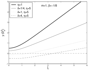
(a) $m=1$, $\beta=-1/8$

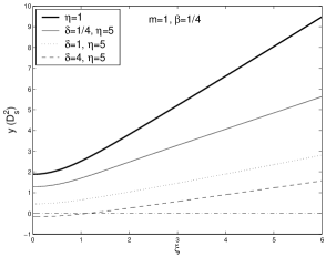
(b) $m=1$, $\beta=1/4$

Figure 10: Five solution curves of $D_{s}^{2}$ from stationary dispersion relation (71) as functions of $\xi$ for $m=1$, $\beta=-1/8,1/4$, $\delta=1/4,\ 1,\ 4$ and $\eta=1,5$. Only the upper $y_{2}$ branches are shown here. For $\eta=1$, solutions $D_{s}^{2}$ are independent of $\delta$.

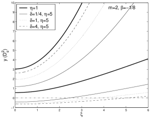
(a) $m=2$, $\beta=-1/8$

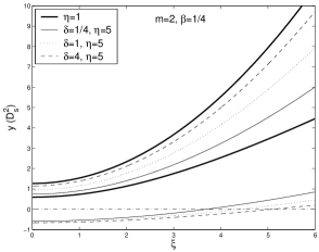
(b) $m=2$, $\beta=1/4$

Figure 11: Two $D_{s}^{2}$ solution branches (given by the same linetype) of stationary dispersion relation (71) for logarithmic spirals with $m=2$, $\beta=-1/8,\ 1/4$, $\delta=1/4,\ 1,\ 4$ and $\eta=1,\ 5$. For $\eta=1$, these solutions are independent of $\delta$. The lower branches are the counterparts of the single-disc case. Note the variation in ordering of two solution branches as $\eta$ changes.

3.2.3 Logarithmic Spiral Configurations with $m\geq 2$

It turns out to be much simpler for $m\geq 2$ cases because when $m\geq 2$, we always have inequalities ${\cal A}_{m}>0$, ${\cal B}_{m}>0$, $0<{\cal C}{\cal N}_{m}<1$, ${\cal H}_{m}>0$ and hence $C_{2}>0$ valid for all ranges of parameters under consideration. This greatly simplifies the analysis, as $y_{1}$ and $y_{2}$ remain to be upper and lower branches, respectively. Meanwhile, we have $Y_{1}^{A}>Y_{1}^{B}>0$ and $Y_{\infty}^{A}>0>Y_{\infty}^{B}=-1$.

For $\eta=1$, we determine

$$\begin{split}&y_{1}=Y_{1}^{A}=\frac{{\cal A}_{m}}{{\cal B}_{m}}>0\ ,\\ &y_{2}=Y_{1}^{B}=\frac{(1-{\cal C}{\cal N}_{m}){\cal A}_{m}}{{\cal H}_{m}}>0\ ;\\ \end{split}$$ (89)

while for $\eta\rightarrow\infty$, we have

$$\begin{split}&y_{1}=Y_{\infty}^{A}=\frac{{\cal A}_{m}[{\cal H}_{m}\delta+(1-{\cal C}{\cal N}_{m}){\cal B}_{m}]}{{\cal B}_{m}{\cal H}_{m}(1+\delta)}>0\ ,\\ &y_{2}=Y_{\infty}^{B}=-1\ .\end{split}$$ (90)

Therefore, the upper $y_{1}$ branch remains always positive, while the lower $y_{2}$ branch first remains positive for small $\eta$ and then becomes negative for $\eta$ greater than a critical $\eta_{c}$ given explicitly by

$$\eta_{c}\equiv 1+\frac{(1-{\cal C}{\cal N}_{m}){\cal A}_{m}(1+\delta)}{[{\cal H}_{m}\delta+(1-{\cal C}{\cal N}_{m}){\cal B}_{m}]}\ .$$ (91)

This critical $\eta_{c}$ always exists for any given $\delta$ because $\eta_{c}$ remains always greater than 1 as dictated by equation (91).

Entirely similar to the aligned $m\geq 2$ cases, the phase relationship between surface mass densities $\mu^{g}$ and $\mu^{s}$ for the upper $y_{1}$ branch of $D_{s}^{2}$ solution is

$$-1<\frac{\mu^{g}}{\mu^{s}}<-\frac{{\cal C}{\cal N}_{m}{\cal A}_{m}\delta}{({\cal H}_{m}\delta+{\cal B}_{m})}\ ,$$ (92)

where the left-hand side corresponds to $\eta=1$ and the right-hand side corresponds to $\eta\rightarrow\infty$. This branch always has out-of-phase relationship between surface mass densities $\mu^{g}$ and $\mu^{s}$ in the range of $\beta\in(-1/4,1/2)$.

Meanwhile for the lower $y_{2}$ branch, the phase relationship between surface mass densities $\mu^{g}$ and $\mu^{s}$ is determined by

$$\delta<\frac{\mu^{g}}{\mu^{s}}<\frac{(1+\delta)}{{\cal C}{\cal N}_{m}}-1\ ,$$ (93)

where the left-hand side corresponds to $\eta=1$ and the right-hand side corresponds to $\eta=\eta_{c}$ where $D_{s}^{2}=y_{2}=0$. This branch always has in-phase relationship between surface mass densities $\mu^{g}$ and $\mu^{s}$ in the prescribed $\beta$ and $\eta$ ranges.

For purpose of illustration, we present in Fig. 11 a few solution examples in terms of $y\equiv D_{s}^{2})$ as functions of ‘radial wavenumber’ $\xi$ for specific parameters $m=2$, $\beta=-1/8$ and $1/4$, $\delta=1/4,\ 1$ and $4$ and $\eta=1$ and $5$.

4 Summary and Discussions

The analysis presented in this paper is a generalization and extension of the previous work by Syer & Tremaine (1996), Shu et al. (2000), Lou & Shen (2003) and Shen & Lou (2003). We have constructed both aligned and logarithmic spiral, scale-free, coplanar stationary perturbation configurations in a composite system of two gravitationally coupled discs. While highly idealized, we have in mind, at least conceptually, is a system of spiral galaxy consisting of one stellar disc and one gaseous disc, with a barotropic equation of state. This problem may then have relevance to distributions of stellar mass and gas materials in a disc galaxy. Qualitatively, the two branches of solutions derived in this paper suggest two possible coupled perturbation modes (not necessarily stationary; see Lou & Fan 1998b) where surface mass density perturbations in the stellar disc and in the gaseous disc exhibit either in-phase or out-of-phase correlations. These two distinctly different classes of perturbation modes are mathematically allowable, although there might be some kind of prevalence related to initial conditions or other uncertainties. For observational diagnostics of disc galaxies, one can obtain non-axisymmetric stellar structures in the optical band (e.g. Rix & Zaritsky 1995) and derive HI maps for the gaseous disc component (e.g. Richter & Sancisi 1994). These two maps in different wave bands may be compared to see whether the stellar and HI gaseous arms are roughly coincident or apparently interlaced. The real situation may be even more complicated than this. Active star formation processes in the optical arms will further consume HI gas and the places where HI gas clumps will trigger more star formation activities. Depending on the level of these interrelated processes, a phase shift between optical arms and HI arms may not be easily interpreted in terms of the out-of-phase perturbation modes. Perhaps, the most cogent evidence for out-of-phase density perturbations would be a lopsided disc galaxy where the gaseous and stellar disc components are comparable and the lopsidednesses for the two components are opposite. In a broader perspective, the ideal two-fluid approach adopted here may be applicable to other two-component disc system where the two components can be treated as ideal fluids with different temperatures, e.g., a composite disc system of stars and dusts or a composite disc system composed of young massive stars and relatively old stars, or even to composite disc systems with more components. These different ‘hot’ and ‘cold’ fluid disc components are coupled in the overall disc dynamics and contribute to various structures in multi-band observations.

In order to satisfy the scale-free conditions in our model, both the stellar and gaseous discs in an axisymmetric equilibrium state have rotation curves $v\propto r^{-\beta}$ and surface mass densities $\Sigma_{0}\propto r^{-1-2\beta}$ with a barotropic index $n=(1+4\beta)/(1+2\beta)$ for the parameter regime of $\beta\in(-1/4,1/2)$. For both cases of aligned and logarithmic spiral perturbations, we derive sensible values of $D_{s}^{2}$ to support such neutral or stationary density wave modes in an inertial frame of reference. There are two classes of stationary density wave modes in a composite system of two coupled discs in general; this is in contrast to one class of stationary density wave modes in a single disc system. We now summarize our main results below.

1. Aligned Stationary Configurations

   For aligned configurations, we focus on the coplanar disturbances whose surface mass densities carry the same cylindrical radial variations of the background equilibrium state.

   The aligned axisymmetric $m=0$ case represents merely a rescaling from one axisymmetric equilibrium to a neighbouring one (Shu et al. 2000; Lou 2002; Lou & Fan 2002; Lou & Shen 2003; Lou & Zou 2004), except that the rescaling here happens in both discs simultaneously.

   In contrast to the eccentric $m=1$ case in a composite system of two gravitationally coupled SIDs with $\beta=0$ (Lou & Shen 2003), the aligned $m=1$ configurations in two coupled scale-free discs with $\beta\neq 0$ are not trivial. Only one branch of $D_{s}^{2}$ solution is physically sensible. For $\beta>-(2^{1/2}-1)/2$, this branch of $D_{s}^{2}$ solution stands as the counterpart of the single-disc case and the surface mass density perturbations in the two discs are in-phase. For $\beta<-(2^{1/2}-1)/2$, this branch of $D_{s}^{2}$ solution has no counterpart of the single-disc case and surface mass density perturbations in the two discs are out-of-phase. There may or may not exist a critical $\eta_{c}$, determined by expression (45), beyond which the $D_{s}^{2}$ solution becomes negative and thus unphysical, depending on the value of $\delta$. Specific classifications and analyses have been presented in subsection 3.1.1.

   For $m\geq 2$ cases, we have derived two branches of solution for possible values of the rotation speed parameter $D_{s}^{2}$ such that aligned stationary perturbation configurations are sustained in a composite disc system. Of the two $D_{s}^{2}$ branches, one is always the upper branch and thus physical for being positive and the coplanar surface mass density perturbations in two discs are out-of-phase (see Lou & Fan 1998). This branch of $D_{s}^{2}$ solution has no counterpart in the case of a single disc. Meanwhile, the other branch of $D_{s}^{2}$ solution stands as the counterpart of the single-disc case with coplanar surface mass density perturbations in the two discs being in-phase. Furthermore, this second branch of $D_{s}^{2}$ solution decreases with increasing $\eta$ and may become negative and thus unphysical when $\eta$ exceeds a critical value $\eta_{c}$ that varies with $\beta$, $m$ and $\delta$ as seen from definition (59). In contrast to the aligned $m=1$ case, this critical $\eta_{c}$ always exists for any values of $\delta$. Details and specific examples can be found in subsection 3.1.2.

2. Stationary Configurations of Logarithmic Spirals

   For unaligned or spiral coplanar perturbations, we consider global logarithmic spiral configurations (Kalnajs 1971; Syer & Tremaine 1996; Shu et al. 2000; Lou 2002; Lou & Fan 2002; Lou & Shen 2003; Lou & Zou 2004).

   For the axisymmetric $m=0$ case with radial oscillations, we have determined the marginal stability curves of $D_{s}^{2}$ versus the ‘radial wavenumber’ $\xi$ for various values of $\beta$. The limiting case of $\eta=1$ reduces to the case of single disc case as if the secondary mode due to the gravitationally coupling between the two discs were absent. The axisymmetric stability criterion is expressed in terms of the stellar rotation parameter $D_{s}^{2}$. Those systems that rotate too slowly will succumb to large-scale instabilities in the collapse regime, while those systems that rotate too fast will fall into the ring-fragmentation regime for short-wavelength instabilities (Safronov 1960; Toomre 1964; Shu et al. 2000; Lou 2002; Lou & Fan 1998, 2002; Lou & Shen 2003; Shen & Lou 2003; Lou & Zou 2004). The stable range of $D_{s}^{2}$ against overall axisymmetric instabilities is expanded for larger $\beta$ values. When $\beta>\beta_{c}\sim 0.436$, the large-scale collapse regime will disappear completely. On the other hand when $\beta<-0.130$, the system cannot be stable at all. The $D_{s}^{2}$ criterion for axisymmetric instabilities with radial oscillations presented here is entirely equivalent to the $w$ parameter used by Syer & Tremaine (1996) for the the case of a full single disc. The composite disc system becomes less stable than the single-disc system. The overall stable $D_{s}^{2}$ range will diminish for larger $\delta$ or $\eta$, while the large-scale collapse instability by itself tends to be suppressed. Specific examples and some analysis techniques are presented in subsection 3.2.1 and Appendixes C and D.

   For the logarithmic spiral case of $m=1$ , the lower branch of $D_{s}^{2}$ solution is always unphysical for being negative and the limiting case of $\eta=1$ corresponds to just the single-disc case. For a given ‘radial wavenumber’ $\xi$, there may or may not exist a critical $\eta_{c}$ beyond which the $D_{s}^{2}$ solution becomes negative, depending on the value of $\delta$. This case is almost identical with the aligned case (III) described in subsection 3.1.1, except for a substitution of ${\cal P}_{1}$ with ${\cal N}_{1}$ and redefinitions for ${\cal A}_{1}$ and ${\cal H}_{1}$. Details and specific examples can be found in subsection 3.2.2.

   For logarithmic spiral cases with $m\geq 2$ , we have obtained analytical results almost in the same forms of the aligned cases. There are two possible values of rotation parameter $D_{s}^{2}$ that can sustain stationary logarithmic spiral configurations in a composite system. Of these two perturbation modes, one has no counterpart in the single-disc case (Lou & Fan 1998) with the surface mass density perturbations in the two discs being out-of-phase, while the other is the counterpart of the single-disc case and has in-phase surface mass density perturbations in the two discs. The out-of-phase mode always exists while the in-phase mode disappears when $\eta$ exceeds a certain critical value $\eta_{c}$ that depends on $\beta$, $m$, $\delta$ and $\xi$ by equation (91). Specific examples can be found in subsection 3.2.3.

3. Non-Axisymmetric Instabilities

   For axisymmetric instabilities it is well established that neutral modes mark the onset of instabilities. We have analytically constructed non-axisymmetric neutral (i.e. stationary) modes for both aligned and logarithmic spiral cases. Do these neutral modes or stationary configurations mark the non-axisymmetric spiral instabilities? Based on transmissions and over-reflections of leading and/or trailing spiral density waves across corotation in a time-dependent analysis, Shu et al. (2000) speculated that the condition for stationary logarithmic spiral configurations in a SID would determine whether spiral density waves could be swing-amplified (Goldreich & Lynden-Bell 1965; Fan & Lou 1997). The criterion of Shu et al. (2000) for swing amplification is consistent with that of Goodman & Evans (1999) in their normal-mode analysis. It is appears worthwhile to pursue the criterion for the onset of non-axisymmetric instabilities in terms of a normal-mode analysis for a composite system that will be performed in a separate paper.

4. Partial Discs

   All computations and discussions above deal with full discs. One can also impose an axisymmetric gravitational potential associated with a background dark matter halo of axisymmetry and ignore disturbances in the dark matter halo caused by coplanar surface mass density perturbations in the composite disc system, that is, the composite system is composed of two partial discs (Syer & Tremaine 1996; Shu et al. 2000; Lou 2002; Lou & Fan 2002; Lou & Shen 2003; Shen & Lou 2003; Lou & Zou 2004). By defining a dimensionless factor $0<{\cal F}<1$ for the ratio of the gravitational potential arising from the two discs together to that of the whole system including the dark matter halo, one may follow the same procedure for full discs to analyze the problem of a composite system of two coupled partial discs. Practically, what one needs to do is to replace all ${\cal P}_{m}$ and ${\cal N}_{m}$ with ${\cal F}{\cal P}_{m}$ and ${\cal F}{\cal N}_{m}$, respectively. The dynamical effect of this background dark matter halo tends to suppress axisymmetric instabilities (Syer & Tremaine 1996; Shu et al. 2000; Lou 2002; Lou & Fan 2002; Lou & Shen 2003; Shen & Lou 2003; Lou & Zou 2004).

5. Magnetized Discs

   By synchrotron radio observations, one can infer spiral magnetic field structures in nearby spiral galaxies (e.g., Lou & Fan 2003 and references therein). It is believed that this is generically true for distant spiral galaxies as well. The presence of magnetic fields in spiral galaxies should affect global star formation rates and thus influence the evolution of disc galaxies. Technically, the interesting problem of including magnetic fields can become quite involved. More specifically, a stellar disc is gravitationally coupled with a magnetized gaseous disc. There are two relatively simple geometries to model configurations of magnetic fields. The first one is the so-called isopedically magnetized configurations (Shu & Li 1997; Shu et al. 2000; Lou & Wu 2004). The second one is to consider coplanar azimuthal magnetic fields with their strengths scaled as powers of cylindrical radius $r$ (Lou 2002; Lou & Fan 2002; Lou & Zou 2004). Now with a more general scale-free disc system investigated in this paper, it would be very interesting to model magnetic fields for both isopedic and azimuthal configurations in a more general composite disc system, a problem also to be presented in a separate paper.

Appendix A Two Real $D_{s}^{2}$ Solutions

We here show that equation (38) always has two different real solutions. The determinant of equation (38) reads

$$\begin{split}\Delta\equiv C_{1}^{2}-4C_{2}C_{0}=\bigg{(}\frac{{\cal A}_{m}+{\cal B}_{m}}{1+\delta}\bigg{)}^{2}\wp\ \end{split}$$ (94)

where

$$\wp\equiv c_{2}\eta^{2}+c_{1}\eta+c_{0}=c_{2}\bigg{(}\eta+\frac{c_{1}}{2c_{2}}\bigg{)}^{2}-\frac{c_{1}^{2}-4c_{0}c_{2}}{4c_{2}}\ ,$$ (95)

and

$$\begin{split}&c_{2}\equiv({\cal B}_{m}+{\cal H}_{m}\delta)^{2}\ ,\\ &c_{1}\equiv 2\delta({\cal H}_{m}-{\cal B}_{m})^{2}-2{\cal B}_{m}{\cal H}_{m}(1+\delta)^{2}\ ,\\ &c_{0}\equiv({\cal H}_{m}+{\cal B}_{m}\delta)^{2}\ .\end{split}$$ (96)

It follows further that

$$\Delta_{1}\equiv c_{1}^{2}-4c_{0}c_{2}=-16{\cal B}_{m}{\cal H}_{m}({\cal H}_{m}-{\cal B}_{m})^{2}\delta(1+\delta)^{2}\ .$$ (97)

Now in the open interval of $\beta\in(-1/4,1/2)$ and for $m\geq 2$, we have $c_{2}>0$, $\Delta_{1}<0$ and thus $\wp>0$ for all $\eta\geq 1$. We have thus proven that $\Delta>0$. While the proof procedure is slightly different for the $m=1$ case, we also can show that $\Delta>0$. It follows that equation (38) always has two different real solutions for $D_{s}^{2}$ corresponding to the upper and lower branches, respectively.

The same proof procedure can be repeated for the logarithmic spiral cases corresponding to stationary dispersion relation (71), which always has $\Delta>0$ for $m\geq 1$. Moreover in the same spirit, we can show $\Delta\geq 0$ for the axisymmetric $m=0$ case. The equal sign corresponds to $({\cal A}_{0}^{\prime}+{\cal B}_{0})=0$.

Appendix B Monotonic Functions

We here provide proofs that the two $D_{s}^{2}$ solutions of dispersion relation (38) for the aligned case and of dispersion relation (71) for logarithmic spiral cases are monotonic functions of $\eta$. Therefore, one can make use of the explicit solutions at $\eta=1$ and in the limit of $\eta\rightarrow\infty$ to well bracket the $D_{s}^{2}$ solution ranges.

First, we rewrite the coefficients $C_{2}$, $C_{1}$ and $C_{0}$ as defined by either expressions (39) for aligned perturbations or expressions (72) for logarithmic spiral perturbations, namely

$$\begin{split}&C_{2}=a_{2}\eta\ ,\\ &C_{1}=a_{1}\eta+b_{1}\ ,\\ &C_{0}=a_{0}\eta+b_{0}\ ,\end{split}$$ (98)

where coefficients $a_{2}$, $a_{1}$, $b_{1}$, $a_{0}$ and $b_{0}$ are determined by directly comparing expressions (39) or (72) of the actual coefficients $C_{2}$, $C_{1}$ and $C_{0}$ that appear in the main text.

With the two $D_{s}^{2}$ solutions explicitly given by $y_{1,2}=(-C_{1}\pm\Delta^{1/2})/2C_{2}$, we have

$$\frac{dy_{1,2}}{d\eta}=\frac{\Delta^{1/2}(C_{1}C_{2}^{\prime}-C_{2}C_{1}^{\prime})+(C_{2}\Delta^{\prime}-\Delta C_{2}^{\prime})}{4C_{2}^{2}\Delta^{1/2}}\ ,$$ (99)

where $\prime$ denotes the derivative with respect to $\eta$ and $\Delta\equiv C_{1}^{2}-4C_{2}C_{0}$ is the determinant that has been proven non-negative in Appendix A.

We next consider to solve equation $y^{\prime}_{1,2}\equiv dy_{1,2}/d\eta=0$ that is equivalent to the following condition

$$4\eta^{2}a_{2}(b_{0}^{2}a_{2}-a_{1}b_{1}b_{0}+a_{0}b_{1}^{2})=0\ .$$ (100)

By straightforward substitutions of the expressions of $a_{2}$, $a_{1}$, $b_{1}$, $a_{0}$, $b_{0}$, this condition turns out to be

$$4\eta^{2}{\cal B}_{m}{\cal H}_{m}\frac{({\cal A}_{m}+{\cal B}_{m})^{4}({\cal H}_{m}-{\cal B}_{m})^{2}\delta}{(1+\delta)^{2}}=0\ ,$$ (101)

which gives only one solution $\eta=0$ for any given sets of $\{m,\ \beta,\ \delta\}$ for aligned perturbations or $\{m,\ \beta,\ \delta,\ \xi\}$ for logarithmic spiral perturbations. Since $dy_{1,2}/d\eta$ are continuous functions of $\eta$, it then follows that for $\eta>1$, $dy_{1,2}/d\eta$ remain either always positive or always negative for any specified sets of $\{m,\ \beta,\ \delta\}$ for aligned perturbations or $\{m,\ \beta,\ \delta,\ \xi\}$ for logarithmic spiral perturbations. In summary, the two $D_{s}^{2}$ solutions $y_{1,2}$ must be monotonic functions of $\eta$ once $\{m,\ \beta,\ \delta\}$ for aligned perturbations or $\{m,\ \beta,\ \delta,\ \xi\}$ for logarithmic spiral perturbations are specified.

Appendix C Properties of ${\cal H}_{\it m}$

We here study the variation of ${\cal H}_{m}$ with respect to $\xi$ in the logarithmic spiral case. For $m>0$, we consider

$$\begin{split}&{\cal A}_{m}=m^{2}+\xi^{2}+1/4+2\beta\ ,\\ &{\cal B}_{m}=(1+2\beta)(m^{2}-2+2\beta)\ ,\\ &{\cal C}=(1+2\beta)/(2\beta{\cal P}_{0})\ ,\\ &{\cal H}_{m}={\cal C}{\cal N}_{m}{\cal A}_{m}+{\cal B}_{m}\ .\end{split}$$ (102)

It is then straightforward to show

$$\frac{d{\cal H}_{m}}{d\xi}={\cal C}{\cal N}_{m}(\Psi_{m}{\cal A}_{m}+2\xi)\ ,$$ (103)

where

$$\begin{split}\Psi_{m}(\xi)&=\frac{i}{2}[\psi(m/2+i\xi/2+1/4)+\psi(m/2-i\xi/2+3/4)\\ &-\psi(m/2-i\xi/2+1/4)-\psi(m/2+i\xi/2+3/4)]\ ,\end{split}$$ (104)

where $\psi$ is the digamma function (or $\psi-$function) defined by $\psi(x)\equiv d[\ln\Gamma(x)]/dx$ with $\Gamma(x)$ being the $\Gamma-$function. In the above derivation, we have used the following relation

$$\frac{d{\cal N}_{m}}{d\xi}={\cal N}_{m}\Psi_{m}\ .$$ (105)

It is also straightforward to show that $\Psi_{m}(\xi>0)$ is negative, $\Psi_{m}(0)=0$ and therefore

$$\frac{d{\cal H}_{m}}{d\xi}\bigg{|}_{\xi=0}=0\ .$$ (106)

Furthermore, we have

$$\begin{split}&\frac{d^{2}{\cal H}_{m}}{d\xi^{2}}\bigg{|}_{\xi=0}>0\ \hbox{for $\beta\in(-1/4,1/2)$}\ ,\\ &\frac{d{\cal H}_{m}}{d\xi}\bigg{|}_{\xi>0}>0\ \hbox{for $\beta\in(-1/4,1/2)$}\ .\end{split}$$ (107)

Therefore, ${\cal H}_{m}$ increases monotonically with increasing $\xi$ and attains its minimum value at $\xi=0$, that is,

$${\cal H}_{m\_min}={\cal H}_{m}|_{\xi=0}={\cal C}{\cal N}_{m}(0){\cal A}_{m}(0)+{\cal B}_{m}\ .$$ (108)

For the $m=0$ case with radial oscillations, we should make the following two replacements

$$\begin{split}&{\cal A}_{0}\rightarrow{\cal A^{\prime}}_{0}=\xi^{2}+1/4\ ,\\ &{\cal H}_{0}\rightarrow{\cal C}{\cal N}_{0}{\cal A^{\prime}}_{0}+{\cal B}_{0}\ ,\end{split}$$ (109)

and repeat the same procedure for $m>0$ cases. The preceding results remain valid. In summary, for $m\geq 0$, ${\cal H}_{m}$ increases monotonically with increasing $\xi$ and attains its minimum value at $\xi=0$. More specifically, we have

$$\begin{split}&{\cal H}_{0\_min}={\cal H}_{0}|_{\xi=0}={\cal C}{\cal N}_{0}(0)(1/4)+(1+2\beta)(-2+2\beta)<0\ ,\\ &{\cal H}_{1\_min}={\cal H}_{1}|_{\xi=0}={\cal C}{\cal N}_{1}(0)(5/4+2\beta)+4\beta^{2}-1>0\ ,\\ &{\cal H}_{m\_min}={\cal H}_{m}|_{\xi=0}={\cal C}{\cal N}_{m}(0){\cal A}_{m}(0)+{\cal B}_{m}>0\ \hbox{for $m\geq 2$\ .}\end{split}$$ (110)

Appendix D

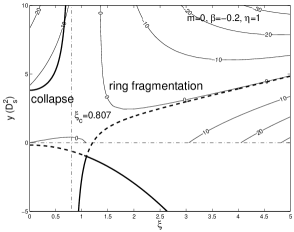
Figure 12: Two branches of $D_{s}^{2}$ solutions to stationary dispersion relation (71) for $m=0$, $\beta=-0.2$ and $\eta=1$. The divergent point is $\xi_{c}=0.807$. In this case of $\eta=1$, the value of $\delta$ can be arbitrary. The system is inevitable to bear ring-fragmentation instabilities and therefore there is no stable range of $D_{s}^{2}$. We also show the deviation from contours of local WKBJ analysis, which are consistent with the global analysis at large ‘radial wavenumber’ $\xi$.

We here discuss more specifically the $m=0$ case with radial oscillations, for which we have

$$\begin{split}&{\cal A^{\prime}}_{0}=\xi^{2}+1/4>0\ ,\\ &{\cal B}_{0}=(1+2\beta)(-2+2\beta)<0\ ,\\ &{\cal C}=(1+2\beta)/(2\beta{\cal P}_{0})\ ,\\ &{\cal H}_{0}={\cal C}{\cal N}_{0}{\cal A^{\prime}}_{0}+{\cal B}_{0}\ .\end{split}$$ (111)

For $\eta=1$ (equivalent to the case of a single disc), the physical $D_{s}^{2}$ solution is

$$Y_{1}^{B}=\frac{(1-{\cal C}{\cal N}_{0}){\cal A^{\prime}}_{0}}{{\cal H}_{0}}>0\ ;$$ (112)

the other $D_{s}^{2}$ solution is negative and thus unphysical. It is noted that for $m\geq 1$, we have $0<{\cal C}{\cal N}_{m}<1$ for all $\xi>0$ and $\beta\in(-1/4,1/2)$. In contrast, the situation of $m=0$ is different, that is, ${\cal C}{\cal N}_{0}$ can be either greater or smaller than 1 and this complicates the analysis.

According to Appendix C, we infer

$$\frac{d({\cal C}{\cal N}_{0})}{d\xi}={\cal C}{\cal N}_{0}\Psi_{0}<0\ \qquad\hbox{for }\qquad\xi>0\ ,$$ (113)

and is equal to zero at $\xi=0$. This implies that ${\cal C}{\cal N}_{0}$ decreases monotonically with increasing $\xi$ and reaches the maximum value at $\xi=0$, namely

$$({\cal C}{\cal N}_{0})_{max}={\cal C}{\cal N}_{0}(0)\bigg{\{}\begin{array}[]{l l}>1\ \qquad\hbox{if $\beta<\beta_{c}\sim 0.436$}\ ,\\ <1\ \qquad\hbox{if $\beta>\beta_{c}\sim 0.436$}\ .\end{array}$$ (114)

Therefore for $\beta<\beta_{c}\sim 0.436$, there is a critical $\xi_{c^{\prime}}$ at which $1-{\cal C}{\cal N}_{0}$ vanishes. If this $\xi_{c^{\prime}}$ coincides with $\xi_{c}$ at which ${\cal H}_{0}$ vanishes, then there is no divergent point for $Y_{1}^{B}$. For this reason, we now check the possibility of $\xi_{c^{\prime}}=\xi_{c}$.

If $\xi_{c^{\prime}}=\xi_{c}$ happens for a specific $\beta_{co}$, the following two equations must be satisfied simultaneously,

$$\begin{split}&(1-{\cal C}{\cal N}_{0})|_{\xi_{c^{\prime}}=\xi_{c}}=0\ ,\\ &({\cal C}{\cal N}_{0}{\cal A^{\prime}}_{0}+{\cal B}_{0})|_{\xi_{c^{\prime}}=\xi_{c}}=0\ ,\end{split}$$ (115)

which gives the relation of $\xi_{c}$ in terms of $\beta_{co}$,

$${\cal A^{\prime}}_{0}+{\cal B}_{0}=\xi_{c}^{2}+1/4+(1+2\beta)(-2+2\beta)=0$$ (116)

and thus

$$\xi_{c}=(7/4+2\beta-4\beta^{2})^{1/2}\ .$$ (117)

Inserting solution (117) into the first equation of (D5), we obtain numerically

$$\beta_{co}\sim-0.130,\ \qquad\qquad\xi_{c^{\prime}}=\xi_{c}\sim 1.193\ .$$ (118)

From the above analysis, we realize that for $\beta_{co}<\beta<1/2$, the axisymmetric marginal stability curves are typical as discussed in subsection 3.2.1. In contrast, for $-1/4<\beta<\beta_{co}$, the axisymmetric marginal stability curves are different and there is no stable range of $D_{s}^{2}$ against overall axisymmetric instabilities, a result also implied in Syer & Tremaine (1996) (see their fig. 2). To see this more clearly, we consider a specific case of $\beta=-0.2$. The divergent point of $Y_{1}^{B}$ is located at $\xi_{c}=0.807$. The stationary configuration for $\eta=1$ (equivalent to the case of a single disc) is shown in Fig. D1.

References

- [1] Balbus S. A., Hawley J. F., 1998, Rev. Mod. Phys., 70, 1
- [2] Berman R. H., Mark J. W.-K., 1977, ApJ, 216, 257
- [3] Bertin G., Lin C. C., 1996, Spiral Structure in Galaxies. MIT Press, Cambridge
- [4] Bertin G., Romeo A. B., 1988, A&A, 195, 105
- [5] Binney J., Tremaine S., 1987, Galactic Dynamics. Princeton University Press, Princeton, New Jersey
- [6] Elmegreen B. G., 1995, MNRAS, 275, 944
- [7] Evans N. W., Read J. C. A., 1998a, MNRAS, 300, 83
- [8] Evans N. W., Read J. C. A., 1998b, MNRAS, 300, 106
- [9] Fan Z.H., Lou Y.-Q., 1996, Nat, 383, 800
- [10] Fan Z. H., Lou Y. Q., 1997, MNRAS, 291, 91
- [11] Goodman J., Evans N. W., 1999, MNRAS, 309, 599
- [12] Goldreich P., Lynden-Bell D., 1965, MNRAS, 130, 125
- [13] Goldreich P., Tremaine S., 1978, Icarus, 34, 240
- [14] Jog C. J., 1996, MNRAS, 278, 209
- [15] Jog C. J., Solomon P. M., 1984a, ApJ, 276, 114
- [16] Jog C. J., Solomon P. M., 1984b, ApJ, 276, 127
- [17] Julian W. H., Toomre A., 1966, ApJ, 146, 810
- [18] Kalnajs A. J., 1971, ApJ, 166, 275
- [19] Kalnajs A. J., 1972, ApJ, 175, 63
- [20] Kalnajs A. J., 1973, Proc. Astron. Soc. Australia, 2, 174
- [21] Lemos J. P. S., Kalnajs A. J., Lynden-Bell D., 1991, ApJ, 375, 484
- [22] Lin C. C., 1987, Selected Papers of C. C. Lin. World Scientific, Singapore
- [23] Lin C. C., Shu F. H., 1964, ApJ, 140, 646
- [24] Lin C. C., Shu F. H., 1966, Proc. Natl Acad. Sci., USA, 73, 3785
- [25] Lou Y.-Q., 2002, MNRAS, 337, 225
- [26] Lou Y.-Q., Fan Z.H., 1998a, ApJ, 493, 102
- [27] Lou Y.-Q., Fan Z. H., 1998b, MNRAS, 297, 84
- [28] Lou Y.-Q., Fan Z.H., 2002, MNRAS, 329, L62
- [29] Lou Y.-Q., Fan Z.H., 2003, MNRAS, 341, 909; astro-ph/0307466
- [30] Lou Y.-Q., Shen Y., 2003, MNRAS, 343, 750; astro-ph/0304270
- [31] Lou Y.-Q., Wu Y., 2004, in preparation
- [32] Lou Y.-Q., Zou Y., 2004, MNRAS, 350, 1220; astro-ph/0312082
- [33] Lynden-Bell D., Kalnajs A. J., 1972, MNRAS, 157, 1
- [34] Lynden-Bell D., Lemos J. P. S., 1993, preprint; astro-ph/9907093
- [35] Lynden-Bell D., Ostriker J. P., 1967, MNRAS, 136, 293
- [36] Mestel L., 1963, MNRAS, 126, 553
- [37] Nicholson, D. R. 1983, Introduction to Plasma Theory, Wiley, New York
- [38] Qian E., 1992, MNRAS, 257, 581
- [39] Richter O.-G., Sancisi R., 1994, A&A, 290, L9
- [40] Rix H.-W., Zaritsky D., 1995, ApJ, 447, 82
- [41] Romeo A. B., 1992, MNRAS, 256, 307
- [42] Safronov V.S., 1960, Ann. Astrophys., 23, 979
- [43] Shen Y., Lou Y.-Q., 2003, MNRAS, 345, 1340; astro-ph/0308063
- [44] Shen Y., Lou Y.-Q., 2004, ChJAA, in press, astro-ph/0404190
- [45] Shen Y., Liu X., Lou Y.-Q., 2004, in preparation
- [46] Shu F. H., Laughlin G., Lizano S., Galli D., 2000, ApJ, 535, 190
- [47] Shu F. H., Li Z.-Y., 1997, ApJ, 475, 251
- [48] Syer D., Tremaine S., 1996, MNRAS, 281, 925
- [49] Toomre A., 1964, ApJ, 139, 1217
- [50] Toomre A., 1977, ARA&A, 15, 437
- [51] Toomre A., 1981, in Structure and Dynamics of Normal Galaxies, ed. S. M. Fall & D. Lynden-Bell (Cambridge: Cambridge Univ. Press), 111
- [52] Zang T. A., 1976, PhD thesis, MIT, Cambridge MA