The very early afterglow powered by ultra-relativistic mildly magnetized outflows

In the Poynting Flux-dominated outflow (the initial ratio of the electromagnetic energy flux to the particle energy flux $\sigma_{0}\gg 1$) model for Gamma-ray bursts, particularly the $\gamma-$ray emission phase, nearly half of the internally dissipated magnetic energy is converted into the $\gamma-$ray energy emission and the rest is converted into the kinetic energy of the outflow. Consequently, at the end of the $\gamma-$ray burst, $\sigma$ decreases significantly ($\sigma\sim 1$ or even smaller). We numerically investigate the very early reverse shock emission powered by such mildly magnetized outflows interacting with medium—uniform interstellar medium (ISM) or stellar wind (WIND). We show that for $\sigma\sim 0.05-1$ and typical parameters of Gamma-ray bursts, both the ISM-ejecta interaction and the WIND-ejecta interaction can power very strong optical emission ($m_{\rm R}\sim 10-12{\rm th}$ magnitude or even brighter). Similar to the very early afterglow powered by the non-magnetized ejecta interacting with the external medium, the main difference between the ISM-ejecta interaction case and the WIND-ejecta interaction case is that, before the reverse shock crosses the ejecta, the R-band emission flux increases rapidly for the former, but for the latter it increases only slightly.

At the very early stage, the ejecta are ultra-relativistic. Due to the beaming effect, the random magnetic field generated in shocks contained in the viewing area is axisymmetric, unless the line of sight is very near the edge of ejecta. The formula $\Pi_{\rm net}\approx 0.60b^{2}/(1+b^{2})$ (where $b$ is the ratio of the ordered magnetic field strength to that of random one) has been proposed to describe the net linear polarization of the synchrotron radiation coming from the viewing area. For $\sigma\sim 0.05-1$, the ordered magnetic field dominates over the random one generated in the reverse shock (As usual, we assume that a fraction $\epsilon_{\rm B}\sim 0.01$ of the thermal energy of the reverse shock has been converted into the magnetic energy), the high linear polarization is expected. We suggest that the linear polarization detection of the early multi-wavelength afterglow is required to see whether the outflows powering GRBs are magnetized or not.

1 Introduction

It is widely accepted that $\gamma$-ray bursts (GRBs) are powered by the dissipation of energy in a highly relativistic wind, driven by gravitational collapse of a massive star into a neutron star or a black hole (see Mészáros 2002 for a recent review). As the observed emission is powered at a distance far from the central source, key questions remain unanswered. One of them is the Gamma-ray burst engines (see Cheng & Lu 2001 for a review). In the standard fireball model, the Gamma-ray burst are powered by the collisions of baryon dominated shells with variable Lorentz factors (Paczyński & Xu 1994; Rees & Mészáros 1994). However, Poynting flux-driven outflows from magnetized rotators is another plausible explantation and there have been various implementations of this concept (Usov 1992, 1994; Thompson 1994; Blackman, Yi & Field 1996; Katz 1997; Mészáros & Rees 1997). The Poynting flux model is in light of the following facts (see Zhang & Mészáros (2004) for a recent review): The Poynting flux outflow can transport a large amount of energy without carrying many baryons. It can alleviate the inefficiency problem of the internal shock model and can also alleviate the magnetic field amplification problem in GRBs and afterglows. It provides the possibility of achieving narrow “peak energy” distributions. In particular, the Poynting flux model provides the most natural explanation so far for the very high linear polarization during the $\gamma$-ray emission phase of GRB 021206 (e.g. Coburn & Boggs 2003; Lyutikov, Pariev & Blandford 2003; Granot 2003; However, see Rutledge & Fox (2004) for argument), although other alternative explanations remain (e.g. Shaviv & Dar 1995; Waxman 2003).

In the past several years, many publications have focused on the dissipation (the energetic non-thermal $\gamma-$ray emission) as well as the acceleration of the Poynting flux outflow (e.g. Usov 1994; Thompson 1994; Smolsky & Usov 1996; Mészáros & Rees 1997; Lyutikov & Blackman 2001; Spruit, Daigne & Drenkhahn 2001; Drenkhahn 2002; Drenkhahn & Spruit 2002). In this paper we turn to investigate the very early reverse shock emission powered by such a magnetized outflow, just as Sari & Piran (1999) and Mészáros & Rees (1999) have done for the baryon dominated fireball. One thing inciting us to do this is that modeling the very early afterglow of GRB 990123 and GRB 021211 suggests the reverse shock emission region is magnetized (Fan et al. 2002; Zhang, Kobayashi & Mészáros 2003).

In the “internal” magnetic dissipation model, GRBs are powered by the magnetic energy dissipation at a radius $r\sim 10^{13}-10^{14}{\rm cm}$. At the end of the $\gamma-$ray burst, a significant fraction of magnetic energy has been dissipated by magnetic reconnection or other processes. Nearly half of the dissipated magnetic energy has been converted into the $\gamma-$ray emission and the rest has been converted into the kinetic energy of the outflow (see Spruit $\&$ Drenkhahn 2003 for a recent review). Consequently, $\sigma$ decreases significantly ($\sim 1$ or even smaller). At a much larger radius, where the outflow begins to be decelerated significantly, the reverse shock emission (the very early afterglow) is expected; this is what we focus on.

At the final stage of the preparation of this manuscript, a paper by Zhang & Kobayashi (2004) appeared. In that paper, the very early reverse shock emission from an arbitrary magnetized ejecta has been analytically investigated.

2 The mild-magnetized outflow

As mentioned before, there are lots of publications focused on the acceleration of the magnetized outflow. One of them is Drenkhahn (2002), in which part of the magnetic energy coupled with the outflow is dissipated internally by reconnection and the Lorentz factor of the flow increases steadily with radius ($\Gamma\propto r^{1/3}$). Here we do not discuss that topic further and just take the numerical example presented in Drenkhahn $\&$ Spruit (2002) as the starting point of our calculation: at the end of the prompt $\gamma-$ray emission phase, the bulk Lorentz factor of the outflow is $\eta\sim 300$; the ratio of the electromagnetic energy flux to the particle energy flux, $\sigma\sim 0.05-1$ (In principle, much lower $\sigma$ is possible, for which the reverse shock emission is similar to that of the usual fireball, which is beyond our interest); the total kinetic energy (including the magnetic energy) is of the order of the typical $\gamma-$ray emission energy, i.e., $E_{\rm kin}\sim 10^{53}{\rm ergs}$.

3 The reverse shock emission

3.1 The dynamical evolution of ejecta

Generally, the dynamical evolution of the ejecta can be divided into two phases—(i) Before the reverse shock crosses the ejecta, i.e., $R<R_{\rm cro}$ ($R$ is the radial coordinate in the burster frame; $R_{\rm cro}$ is the radius at which the reverse shock crosses the ejecta); at that time two shocks exist. The dynamical evolution of the ejecta is governed by the jump condition of shocks (e.g., Blandford & McKee 1976; Sari & Piran 1995); (ii) After the reverse shock crosses the ejecta, i.e., $R>R_{\rm cro}$, in this case only the forward shock exists. The hydrodynamical evolution can be calculated by taking the generic dynamical model of GRB remnants (e.g., Huang, Dai & Lu 1999; Huang et al. 2000; Feng et al. 2002).

3.1.1 The dynamical evolution for $R<R_{\rm cro}$

Similar to Sari & Piran (1995), the dynamical evolution of the ejecta is obtained by solving the jump condition for strong shocks. For the ejecta interacting with the external medium, there are two shocks formed, one is the forward shock expanding into the medium, the other is the reverse shock penetrating the ejecta. There are four regions in this system: (1) The un-shocked medium; (2) The shocked medium; (3) The shocked ejecta material; (4) The un-shocked ejecta material. The medium is at rest relative to the observer. The bulk Lorentz factors $\Gamma_{\rm j}$ ($j=1,4$, $\Gamma_{4}\equiv\eta$) and the corresponding velocities $\beta_{\Gamma_{\rm j}}=(1-1/\Gamma_{\rm j}^{2})^{1/2}$ are measured by the observer. Thermodynamic quantities: $n_{\rm j}$, $p_{\rm j}$, $e_{\rm j}$, $B^{\prime}_{\rm j}$ (particle number density, pressure, internal energy density, magnetic field strength) are measured in the fluids’ rest frame (we assume the un-shocked ejecta and medium are cold, i.e., $e_{4}=e_{1}=0$), so is the $p_{\rm B,i}$ (the magnetic pressure). The equations governing the forward shock are (Blandford $\&$ Mackee 1976)

$$n_{2}/n_{1}=4\Gamma_{2}+3,e_{2}/n_{2}=(\Gamma_{2}-1)m_{p}c^{2}.$$ (1)

Below, following Kennel & Coroniti (1984, hereafter KC84) we try to derive the ($90^{\rm o}$) shock jump condition governing the reverse shock with the MHD conservation laws by assuming the magnetic field frozen in the outflow is nearly toroidal (KC84):

$$n_{4}u_{4}=n_{3}u_{3},$$ (2)

$$\gamma_{4}\mu_{4}+{EB_{4}\over 4\pi n_{4}u_{4}}=\gamma_{3}\mu_{3}+{EB_{3}\over 4\pi n_{4}u_{4}},$$ (3)

$$\mu_{4}u_{4}+{P_{4}\over n_{4}u_{4}}+{B_{4}^{2}\over 8\pi n_{4}u_{4}}=\mu_{3}u_{3}+{P_{3}\over n_{4}u_{4}}+{B_{3}^{2}\over 8\pi n_{4}u_{4}},$$ (4)

where $B_{\rm i}$ and $E$ denote the shock frame magnetic and electric fields respectively, $E=u_{4}B_{4}/\gamma_{4}=u_{3}B_{3}/\gamma_{3}$. $\gamma_{\rm i}$ ($i=3,\leavevmode\nobreak\ 4$) is the Lorentz factor of the fluid measured in the reverse shock frame, $u_{\rm i}^{2}=\gamma_{\rm i}^{2}-1$, $\beta_{\rm i}=u_{\rm i}/\gamma_{\rm i}$. $\mu$ is the specific enthalpy, which is defined by $\mu_{\rm i}=m_{\rm p}c^{2}+\hat{\gamma}_{\rm i}P_{\rm i}/[(\hat{\gamma}_{\rm i}-1)n_{\rm i}]$ for a gas with an adiabatic index $\hat{\gamma_{\rm i}}$.

Solving equation (3) for $\mu_{3}$ and inserting the resulting expression into equation (4) leads to

$$\sigma(Y^{2}-1) + {2[1+\sigma(1-Y)]\over u_{3}\gamma_{3}}{u_{4}\over\gamma_{4}}[u_{3}^{2}+{\hat{\gamma}_{3}-1\over\hat{\gamma}_{3}}]-2({u_{4}\over\gamma_{4}})^{2}$$ (5)

$$- {2P_{4}\over n_{4}\mu_{4}\gamma_{4}^{2}}-{u_{4}\over u_{3}}{2(\hat{\gamma}_{3}-1)m_{\rm p}c^{2}\over\hat{\gamma}_{3}\mu_{4}\gamma_{4}^{2}}=0,$$

where $\sigma\equiv{B_{4}^{2}/[4\pi n_{4}\mu_{4}\gamma_{4}^{2}]}$ and $Y\equiv{\gamma_{3}u_{4}\over\gamma_{4}u_{3}}$. With equation (3), the downstream pressure $P_{3}$ can be calculated as follows:

$$P_{3}={\hat{\gamma}_{3}-1\over\hat{\gamma}_{3}}[{\gamma_{4}\over\gamma_{3}}(1+\sigma(1-Y))-{m_{\rm p}c^{2}\over\mu_{4}}]n_{3}\mu_{4}.$$ (6)

For $\gamma_{4}\gg 1$ and $P_{4}=0$, equation (5) can be arranged into (Assuming $2(\hat{\gamma}_{3}-1)/u_{3}\hat{\gamma}_{3}\gamma_{4}$ can be ignored)

$${(1+\sigma)(2-\hat{\gamma}_{3})\over\hat{\gamma}_{3}}u_{3}^{4}+[{\hat{\gamma}_{3}-4\over 4\hat{\gamma}_{3}}\sigma^{2}-{\hat{\gamma}_{3}^{2}-2\hat{\gamma}_{3}+2\over\hat{\gamma}_{3}^{2}}\sigma$$

$$\leavevmode\nobreak\ \leavevmode\nobreak\ \leavevmode\nobreak\ \leavevmode\nobreak\ \leavevmode\nobreak\ -({\hat{\gamma}_{3}-1\over\hat{\gamma}_{3}})^{2}]u_{3}^{2}+({\hat{\gamma}_{3}-2\over 2\hat{\gamma}_{3}})^{2}\sigma^{2}=0.$$ (7)

For $\hat{\gamma}_{3}=4/3$, the above equation can be greatly simplified

$$8(1+\sigma)u_{3}^{4}-(8\sigma^{2}+10\sigma+1)u_{3}^{2}+\sigma^{2}=0,$$ (8)

whose solution is equation (4.11) of KC84.

The total pressure in region 3 can be calculated by $P_{\rm 3,tot}=P_{3}+{u_{4}^{2}{B^{\prime}}_{\rm 4}^{2}\over 8\pi u_{3}^{2}}$. The equality of pressure and velocities along the contact discontinuity yields $P_{\rm 3,tot}=P_{2}={4\Gamma_{2}^{2}n_{1}m_{\rm p}c^{2}/3},\leavevmode\nobreak\ \Gamma_{2}=\Gamma_{3}$. For the Lorentz factor of the reverse shock (measured by the observer) $\Gamma_{\rm rsh}\gg 1$, $\gamma_{\rm 4}$ can be expressed as $\gamma_{4}\approx(\eta/\Gamma_{\rm rsh}+\Gamma_{\rm rsh}/\eta)/2$, which in turn yields $\Gamma_{\rm rsh}\approx(\gamma_{4}-u_{4})\eta$. On the other hand, $\gamma_{\rm 3}$ can be expressed as $\gamma_{3}\approx(\Gamma_{2}/\Gamma_{\rm rsh}+\Gamma_{\rm rsh}/\Gamma_{2})/2$, which in turn yields $\Gamma_{\rm 2}\approx(\gamma_{3}+u_{3})\Gamma_{\rm rsh}$, where the relation $\Gamma_{2}=\Gamma_{3}$ has been taken. Combing these relations we have $\Gamma_{2}\approx(\gamma_{3}+u_{3})(\gamma_{4}-u_{4})\eta$. Finally, we have the equation (the equality of pressure)

$${{B^{\prime}}_{\rm 4}^{2}\over 4\pi\sigma}\{{u_{4}\over u_{3}}{(\hat{\gamma}_{3}-1)\over\hat{\gamma}_{3}}[{\gamma_{4}\over\gamma_{3}}(1+\sigma(1-Y))-{m_{\rm p}c^{2}\over\mu_{4}}]+{\sigma u_{4}^{2}\over 2u_{3}^{2}}\}$$

$$={4[(\gamma_{3}+u_{3})(\gamma_{4}-u_{4})\eta]^{2}n_{1}m_{\rm p}c^{2}\over 3},$$ (9)

where $B^{\prime}_{4}=2.6\times 10^{20}{\rm G}\leavevmode\nobreak\ R^{-1}\eta^{-1}$. Equations (1), (5) and (9) are our basic formulae, with which we can calculate the dynamical evolution of the magnetized outflow interacting with the medium, and then the reverse shock emission. However, these equations cannot be solved analytically unless $\sigma\gg 1$. For $\sigma\sim 1$ or smaller, only the numerical calculation can be performed, which is to be presented at the end of this section.

$R_{\rm cro}$ can be determined as follows: $\beta_{\rm rsh}$, the velocity of the reverse shock in the observer’s frame, can be parameterized as (Sari $\&$ Piran 1995)

$$\beta_{\rm rsh}={\Gamma_{3}n_{3}\beta_{\rm\Gamma_{3}}-\Gamma_{4}n_{4}\beta_{\rm\Gamma_{4}}\over{\Gamma_{3}n_{3}-\Gamma_{4}n_{4}}}.$$ (10)

Differentially, $(\beta_{\rm\Gamma_{4}}-\beta_{\rm rsh})dR=d\Delta$, where $\Delta$ is the width of the reverse shock penetrating into the ejecta measured by the observer. $R_{\rm cro}$ is determined by $\int d\Delta=\int_{0}^{\rm R_{\rm cro}}(\beta_{\rm\Gamma_{4}}-\beta_{\rm rsh})dR=\Delta_{0}$, where $\Delta_{0}$ is the width of the ejecta measured by the observer, which can be estimated as $\Delta_{0}\approx cT_{90}/(1+z)$ ($T_{90}$ is the observed duration of GRBs).

3.1.2 The dynamical evolution for $R>R_{\rm cro}$

After the reverse shock has crossed the ejecta, only the forward shock exists, whose dynamics have been discussed in great detail (e.g. Huang et al. 1999; Huang et al. 2000; Panaitescu & Kumar 2001; Feng et al. 2002). However, in the current work, the ejecta is magnetized and how to convent the magnetic energy into kinetic energy is poorly known. But the energy conservation must be satisfied. As a zeroth order approximation, here we take Huang et al.’s (1999) differential equation to depict the dynamical evolution of the magnetized ejecta

$${d\Gamma\over dm}=-{\Gamma^{2}-1\over M^{\prime}_{\rm ej}+\epsilon m+2(1-\epsilon)\Gamma m}.$$ (11)

where $\Gamma$ is the bulk Lorentz factor of the outflow, $\beta=(1-1/\Gamma^{2})^{1/2}$ is the corresponding velocity in unit of light speed; $m$ is the mass of the medium swept by the ejecta, $dm=4\pi R^{2}n_{1}m_{\rm p}dR$; $0<\epsilon\leq 1$ is the radiation efficiency; $M^{\prime}_{\rm ej}$ is determined by (the energy conservation) $\gamma_{\rm cro}M^{\prime}_{\rm ej}c^{2}=(1-\epsilon_{\rm rad})E_{0}$, where $\epsilon_{\rm rad}$ is the fraction of total energy radiated for $R\leq R_{\rm cro}$, $E_{0}$ is the initial isotropic energy of the ejecta. $\gamma_{\rm cro}$ is the bulk Lorentz factor of the ejecta at $R_{\rm cro}$, which can be determined by equations (1), (5) and (9).

3.2 The synchrotron radiation

3.2.1 Electron distribution

In the absence of radiation loss, the distribution of the shock accelerated electrons behind the blastwave is usually assumed to be a power law function of electron energy, i.e.,

$$\frac{dN_{\rm e}^{\prime}}{d\gamma_{\rm e}}\propto\gamma_{\rm e}^{-p},\,\,\,\,\,\,(\gamma_{\rm e,m}\leq\gamma_{\rm e}\leq\gamma_{\rm e,M}),$$ (12)

where $p\approx 2.2$, $\gamma_{\rm e,M}=10^{8}(B^{\prime}/1{\rm G})^{-1/2}$ is the maximum Lorentz factor (Dai, Huang & Lu 1999), where $B^{\prime}$ is the comoving frame magnetic field strength. As usual, for material heated by the forward shock, we assume the magnetic energy density in the comoving frame is a fraction $\epsilon_{\rm B}$ of the total thermal energy, $B_{2}^{\prime}$ can be estimated as

$$\frac{B_{\rm 2}^{\prime 2}}{8\pi}=\epsilon_{\rm B}(4\gamma^{\prime}_{2}+3)(\gamma^{\prime}_{2}-1)n_{1}m_{\rm p}c^{2},$$ (13)

where $\gamma^{\prime}_{2}=\Gamma_{2}$ for $R<R_{\rm cro}$ and $\gamma^{\prime}_{2}=\Gamma$ for $R>R_{\rm cro}$. For region 3 ($R\leq R_{\rm cro}$), $B^{\prime}_{3}=u_{4}B^{\prime}_{4}/u_{3}$.

Similarly, for region 2 and 3, the thermal energy of electrons in the comoving frame is assumed to be a fraction $\epsilon_{\rm e}$ of the total thermal energy, then $\gamma_{\rm e,m}$ can be estimated by

$$\gamma_{\rm e,m}=\epsilon_{\rm e}\frac{p-2}{p-1}\frac{m_{\rm p}}{m_{\rm e}}(\gamma^{\prime}-1),$$ (14)

where $m_{\rm e}$ is the rest mass of electron, $\gamma^{\prime}=\gamma^{\prime}_{2}$ for region 2 and $\gamma^{\prime}=\gamma_{\rm p,th}+1$ for region 3, where the thermal Lorentz factor of the shocked proton $\gamma_{\rm p,th}$ can be estimated by (see equation (6))

$$\gamma_{\rm p,th}\equiv e_{3}/n_{3}m_{\rm p}c^{2}\approx{1\over\hat{\gamma}_{3}}[{\gamma_{4}\over\gamma_{3}}(1+\sigma(1-Y))-{m_{\rm p}c^{2}\over\mu_{4}}]{\mu_{4}\over m_{\rm p}c^{2}}.$$ (15)

It is well known that radiation loss may play an important role in the process. Sari, Piran & Narayan (1998) have derived an equation for the critical electron Lorentz factor, $\gamma_{\rm c,k}$ ($k=2,3$ represent region 2 and 3), above which synchrotron radiation is significant

$$\gamma_{\rm c,k}=\frac{12\pi m_{\rm e}\Gamma^{\prime}(1-\beta^{\prime}\mu)c}{\sigma_{\rm T}B_{\rm k}^{\prime 2}t},$$ (16)

where $t$ is the observer time, $\mu\equiv\cos\Theta$, $\Theta$ is the angle between the velocity of emitting material and the line of sight; Throughout the rest of this work, $\Gamma^{\prime}=\Gamma_{2}$ ($\beta^{\prime}$ is the corresponding velocity in unit of light) in the presence of reverse shock and $\Gamma^{\prime}=\Gamma$ at later time. If the emitting material moves on the line of sight, equation (16) reduces to the familiar form $\gamma_{\rm c,k}=\frac{6\pi m_{\rm e}c}{\sigma_{\rm T}\Gamma^{\prime}B_{\rm k}^{\prime 2}t}$. For electrons with Lorentz factors below $\gamma_{\rm c,k}$, the synchrotron radiation is ineffective. For electrons above $\gamma_{\rm c,k}$, they are highly radiative.

In the presence of steady injection of electrons accelerated by the shock, the distribution of electrons with $\gamma_{\rm e}>\gamma_{\rm c,k}$ has a power law function with an index of $p+1$ (Rybicki & Lightman 1979), while the distribution of adiabatic electrons is unchanged. The actual distribution should be given according to the following cases:

(i) For $\gamma_{\rm c}\leq\gamma_{\rm e,m}\leq\gamma_{\rm e,M}$, i.e., the fast cooling phase

$$\frac{dN_{\rm e}^{\prime}}{d\gamma_{\rm e}}=C_{1}\left\{\begin{array}[]{ll}\gamma_{\rm e}^{-2}\,,&(\gamma_{\rm c}\leq\gamma_{\rm e}\leq\gamma_{\rm e,m}),\\ \gamma_{\rm e,m}^{p-1}\gamma_{\rm e}^{-(p+1)}\,,&(\gamma_{\rm e,m}<\gamma_{\rm e}\leq\gamma_{\rm e,M}),\end{array}\right.$$ (17)

$$C_{1}=[{1\over\gamma_{\rm c}}-{p-1\over p}{1\over\gamma_{\rm e,m}}-{\gamma_{\rm m}^{\rm p-1}\gamma_{\rm e,M}^{\rm-p}\over p}]^{-1}N_{\rm tot}\,,$$ (18)

where $N_{\rm tot}$ is the total number of radiating electrons involved.

(ii) For $\gamma_{\rm e,m}<\gamma_{\rm c}\leq\gamma_{\rm e,M}$, i.e., the slow cooling phase

$$\frac{dN_{\rm e}^{\prime}}{d\gamma_{\rm e}}=C_{2}\left\{\begin{array}[]{ll}\gamma_{\rm e}^{-p}\,,&(\gamma_{\rm e,m}\leq\gamma_{\rm e}\leq\gamma_{\rm c}),\\ \gamma_{\rm c}\gamma_{\rm e}^{-(p+1)}\,,&(\gamma_{\rm c}<\gamma_{\rm e}\leq\gamma_{\rm e,M}),\end{array}\right.$$ (19)

where

$$C_{2}=[{\gamma_{\rm e,m}^{\rm 1-p}\over p-1}-{\gamma_{\rm c}^{\rm 1-p}\over p(1-p)}-{\gamma_{\rm c}\gamma_{\rm e,M}^{\rm-p}\over p}]^{-1}N_{\rm tot}.$$ (20)

As the reverse shock has crossed the ejecta, there are no freshly heated electrons injected and the ejecta cools adiabatically. Here we investigate the decay of the magnetic field and the cooling behavior of electrons. In the current case, the magnetic field is ordered and satisfies the magnetic flux conservation. As usual, the ejecta are in the spreading phase and the width can be estimated as $\Delta^{\prime}\sim R/\Gamma$. Therefore, $B_{3}^{\prime}\propto R^{-1}\Gamma^{-1}/\Delta^{\prime}\propto R^{-2}$. The cooling behavior of electrons is more difficult to estimate. Here we simply assume the cooling of electrons is not much different from that of the non-magnetized case. According to Mészáros & Rees (1999), $\gamma_{\rm e,m}\propto R^{\rm-(9-s)/6}$ (so does $\gamma_{\rm c}$, since all of them cool by adiabatic expansion only), where $s=0$ for the ISM and $s=2$ for the stellar wind. In the case of fast cooling, once $\nu_{\rm c,obs}=eB^{\prime}_{3}\gamma_{\rm c}^{2}\Gamma_{3}/2\pi m_{\rm e}c$ drops below the observed frequency, the flux drops exponentially with time (Sari & Piran 1999). If the equal arriving time surface has been taken into account, the flux drops more slowly.

3.2.2 Relativistic transformations

In the co-moving frame, synchrotron radiation power at frequency $\nu^{\prime}$ from electrons is given by (Rybicki & Lightman 1979)

$$P^{\prime}(\nu^{\prime})=\frac{\sqrt{3}e^{3}B^{\prime}}{m_{\rm e}c^{2}}\int_{\gamma^{\prime}_{\rm e}}^{\gamma_{\rm e,M}}\left(\frac{dN_{\rm e}^{\prime}}{d\gamma_{\rm e}}\right)F\left(\frac{\nu^{\prime}}{\nu_{\rm c}^{\prime}}\right)d\gamma_{\rm e},$$ (21)

where $e$ is electron charge, $\nu_{\rm c}^{\prime}=3\gamma_{\rm e}^{2}eB^{\prime}/(4\pi m_{\rm e}c)$, $\gamma^{\prime}_{\rm e}=\min\{\gamma_{\rm e,m},\gamma_{\rm c}\}$ and

$$F(x)=x\int_{x}^{+\infty}K_{5/3}(k)dk,$$ (22)

with $K_{5/3}(k)$ being the Bessel function. We assume that this power is radiated isotropically in the comoving frame, $\frac{dP^{\prime}(\nu^{\prime})}{d\Omega^{\prime}}=\frac{P^{\prime}(\nu^{\prime})}{4\pi}$.

The angular distribution of power in the observer’s frame is (Rybicki & Lightman 1979; see also Huang et al. 2000)

$$\frac{dP(\nu)}{d\Omega}=\frac{1}{\Gamma^{\prime 3}(1-\beta^{\prime}\mu)^{3}}\frac{dP^{\prime}(\nu^{\prime})}{d\Omega^{\prime}}=\frac{1}{\Gamma^{\prime 3}(1-\beta^{\prime}\mu)^{3}}\frac{P^{\prime}(\nu^{\prime})}{4\pi},$$ (23)

$$\nu=\frac{\nu^{\prime}}{(1+z)\Gamma^{\prime}(1-\beta^{\prime}\mu)},$$ (24)

where $z$ is the redshift of the ejecta. Then the observed flux density at frequency $\nu$ is

$$S_{\nu} = \frac{1}{A}\left(\frac{dP(\nu)}{d\Omega}\frac{A}{D_{\rm L}^{2}}\right)$$ (25)

$$= \frac{1+z}{{\Gamma^{\prime}}^{3}(1-\beta^{\prime}\mu)^{3}}\frac{1}{4\pi D_{\rm L}^{2}}P^{\prime}\left((1+z)\Gamma^{\prime}(1-\beta^{\prime}\mu)\nu\right),$$

where $A$ is the area of our detector and $D_{\rm L}$ is the luminosity distance (we assume $H_{0}=65\rm km$ $\rm s^{-1}$ $\rm Mpc^{-1}$, $\Omega_{M}=0.3$, $\Omega_{\wedge}=0.7$).

3.2.3 Equal arrival time surfaces

Photons received by the detector at a particular time $t$ are not emitted simultaneously in the burster frame. In order to calculate observed flux densities, we should integrate over the equal arrival time surface determined by (e.g. Huang et al. 2000)

$$t=\int\frac{1-\beta^{\prime}\mu}{\beta^{\prime}c}dR\equiv{\rm const},$$ (26)

within the boundaries.

3.3 Numerical results

In our calculation, the number density of the medium (in unit of $\rm cm^{-3}$) has been taken as

$$n_{1}=\left\{\begin{array}[]{ll}{\rm const.}\,,&({\rm ISM}),\\ 3.0\times 10^{35}A_{*}R^{-2}\,,&({\rm WIND}),\end{array}\right.$$ (27)

respectively, where $A_{*}=\frac{\dot{M}}{10^{-5}M_{\odot}\leavevmode\nobreak\ \rm yr^{-1}}(\frac{v_{\rm w}}{10^{3}{\rm km\leavevmode\nobreak\ s^{-1}}})^{-1}$, $\dot{M}$ is the mass loss rate of the progenitor, $v_{\rm w}$ is the wind velocity (Dai & Lu 1998; Chevalier & Li 2000). In our numerical calculation, we take $A_{*}=1$.

For illustration, we take $E_{\rm kin}=10^{53}{\rm ergs}$, $z=1$, $L=2\times 10^{51}{\rm ergs\leavevmode\nobreak\ s^{-1}}$ (equally, $T_{90}=50(1+z){\rm s}$), $\eta=300$, $p=2.2$, $P_{4}=0$ and $\epsilon_{\rm e}=0.3$. In the case of ISM-ejecta interaction, the protons in the region 3 are only mild-relativistic or even sub-relativistic, but electrons are ultra-relativistic, so $\hat{\gamma}_{3}=13/9$. In the case of WIND-ejecta interaction, protons heated by the reverse shock are relativistic, so $\hat{\gamma}_{3}=4/3$.

3.3.1 ISM-ejecta interaction case

The sample very early R-band ($\nu_{\rm R}=4.6\times 10^{14}{\rm Hz}$) light curves have been shown in figure 1. Before the reverse shock crosses the ejecta, electrons accelerated by the reverse shock are in the slow cooling phase and the synchrotron emission at R-band increases rapidly with time. At tens of seconds after the main burst, the reverse shock emission at R band is bright to $m_{\rm R}\sim 10-12{\rm th}$ magnitude and the forward shock emission is relatively dimmer. Therefore, the very early reverse shock emission can be detected independently. After the reverse shock has crossed the ejecta, there are no freshly accelerated electrons injected and the R-band emission drops sharply.

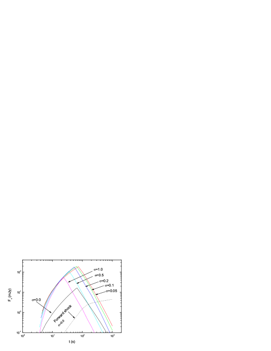
Figure 1: The very early R-band ($\nu_{\rm R}=4.6\times 10^{14}{\rm Hz}$) light curve powered by the mildly magnetized outflow (the degrees of the magnetization have been marked in the figure) interacting with the interstellar medium. The parameters taken in the calculation are: $z=1$, $E_{\rm kin}=10^{53}{\rm ergs}$, $L=2\times 10^{51}{\rm ergs\leavevmode\nobreak\ s^{-1}}$, $\eta=300$, $n_{1}=1{\rm cm^{-3}}$, $\epsilon_{\rm e}=0.3$ and the radiation efficiency $\epsilon=\epsilon_{\rm e}$. For $\sigma=0$ and the forward shock, it is assumed that $\epsilon_{\rm B}=0.01$.

In figure 1, there are two interesting phenomena: (i) The peak flux at R-band increases with the increasing $\sigma$ for $\sigma<0.1$, but for $\sigma>0.1$ the peak flux at R-band decreases with the increasing $\sigma$ (A similar result has been obtained by Zhang & Kobayashi 2004). This behavior can be understood as follows: For $\sigma\ll 1$, the electrons heated by the reverse shock is in slow cooling phase. At $R_{\rm cro}$, the typical synchrotron radiation frequency $\nu_{\rm m,obs}=\Gamma_{2}\gamma_{\rm e,m}^{2}eB^{\prime}_{3}/[2\pi(1+z)m_{\rm e}c]$ is much lower than $\nu_{\rm R}$, as is $\nu_{\rm c,obs}$. We have approximately $F_{{\rm\nu_{\rm R}}}\propto{B^{\prime}_{3}}^{(p-1)/2}$. Roughly speaking, the observed flux increases with the increasing $\sigma$. For larger $\sigma$, the reverse shock has been suppressed and the electrons involved in the emission decrease. So $F_{\rm\nu_{\rm R}}$ drops again (see Zhang & Kobayashi 2004 for more detailed explanation). (ii) For $\sigma\sim 1$, the crossing time $t_{\rm cro}$ (at which the reverse shock crosses the ejecta; in figures 1 and 2, it equals the peak time of the reverse shock emission) is much shorter than $T_{90}$. Here we explain this in some detail. In the presence of reverse shock, differentially, $t_{\rm cro}$ satisfies

$$dt_{\rm cro}=(1+z)\frac{1-\beta_{\rm\Gamma_{3}}}{\beta_{\rm\Gamma_{4}}-\beta_{\rm rsh}}\frac{d\Delta}{c}\approx(1+z)\frac{\Gamma_{\rm rsh}^{2}}{\Gamma_{3}^{2}}\frac{d\Delta}{c}.$$ (28)

With $\Gamma_{\rm rsh}\approx(\gamma_{3}-u_{3})\Gamma_{3}$, we have $dt_{\rm cro}\approx\frac{1+z}{(\gamma_{3}+u_{3})^{2}}\frac{d\Delta}{c}$. Approximately

$$t_{\rm cro}=\int{dt_{\rm cro}}\approx\frac{1}{(\gamma_{\rm 3,cro}+u_{\rm 3,cro})^{2}}T_{90},$$ (29)

where $\gamma_{\rm 3,cro}$ and $u_{\rm 3,cro}$ are the corresponding value of $\gamma_{3}$ and $u_{3}$ at $R_{\rm cro}$. In the case of non-magnetization and the reverse shock is relativistic, $\gamma_{\rm 3,cro}\approx\sqrt{9/8}$, which yields $t_{\rm cros}\approx(1+z)\Delta_{0}/2c\approx T_{\rm 90}/2$ (This result coincides with the “classical” result of Sari & Piran 1995). While for $\sigma=1$, $\gamma_{\rm 3,cro}\approx 1.37$ which results in $t_{\rm cros}\approx T_{\rm 90}/5$, which is quite consistent with our numerical result in Fig.1. Equation (29) applies to the following WIND-ejecta interaction case as well, if only the reverse shock is relativistic or at least mild-relativistic.

3.3.2 WIND-ejecta interaction case

In the case of WIND-ejecta interaction (see figure 2), before the reverse shock crosses the ejecta, the electrons accelerated by the reverse shock are in fast cooling phase and the R-band emission increases only slightly with time. This temporal behavior is very similar to that of non-magnetized fireball case (See Wu et al. (2003) for an analytical investigation). At $t_{\rm cro}$, the reverse shock emission at R band is very bright ($m_{\rm R}\sim 9-10{\rm th}$ magnitude) and the forward shock emission is relatively dimmer. Therefore, the very early reverse shock emission can be detected independently, too. After the reverse shock has crossed the ejecta, the R-band emission drops sharply.

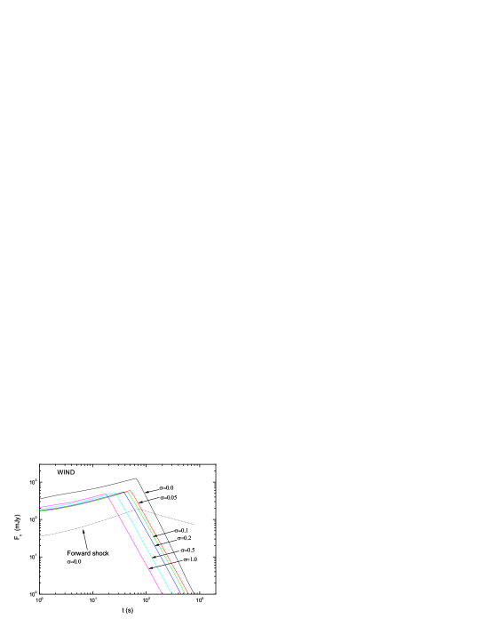
Figure 2: The very early R-band light curve powered by the mildly magnetized outflow (the degree of the magnetization has been marked in the figure) interacting with the stellar wind. The parameters taken here are the same to those of figure 1 except $n_{1}=3\times 10^{35}R^{-2}{\rm cm^{-3}}$.

Since the current reverse shock is relativistic, as implied by equation (29), $t_{\rm cro}$ decreases with increasing $\sigma$. However, in figure 2, the R-band reverse shock emission is brightest at $\sigma=0$, which seems to be inconsonant with the result shown in figure 1. The main reason for this “divergence” is: For $R<10^{17}{\rm cm}$, the WIND is far denser than the ISM. Consequently, the reverse shock is very strong and the ejecta has been decelerated significantly at a radius $\sim 3\times 10^{15}{\rm cm}$ (Note that in the case of ISM-ejecta interaction, the corresponding radius is $\sim 10^{17}{\rm cm}$). Even for $\sigma=0$, the electrons heated by the reverse shock are in the fast cooling phase and $\nu_{\rm m,obs}$ is much higher than the observer frequency $\nu_{\rm R}$. With the increasing $\sigma$, the corresponding $R_{\rm cro}$ decreases. As a result, $B^{\prime}_{3}$ increases. However, now $F_{\rm\nu_{\rm R}}\propto{B^{\prime}_{3}}^{-1/2}$. Consequently, the reverse shock emission powered by the high $\sigma$ ejecta interacting with WIND is dimmer than that powered by the low $\sigma$ ones.

4 The linear polarization

It is well known that for the totally ordered magnetic configuration, high linear polarization is expected. For the random magnetic configuration, mild linear polarization can be expected if some specific geometry effects have been taken into account. Sometimes the magnetic field is not only ordered or only random. Then it is interesting to investigate its linear polarization. Here we propose a simple formula to describe the linear polarization properties of a slab of such a mixed magnetic field, with which we can see the impact of the ordered field on the polarization.

Following Laing (1980; See his Appendix A1 for detail), the coordinates involved are defined as follows ( see figure 3):

Figure 3: Coordinates used in the calculation of the polarization properties of a slab of mixed field (after Laing 1980).

$\alpha$ is the angle between the plane of the ejecta and the line of sight; $x$, $y$, $z$ are rectangular coordinates with the z-axis pointing towards the observer (i.e., the direction n) and the y-axis parallel to the “local” plane of the ejecta; $x^{\prime}$, $y^{\prime}$ are coordinates in the plane of the ejecta, $y^{\prime}$ is parallel to y; $\theta$ is the angle between the field direction and the $x^{\prime}$ axis at any point in the ejecta; $\chi$ is the position angle of the E-vector of the polarized radiation, measured from the $x-y$ plane. Therefore the random (ordered) magnetic-field vector $\textbf{B}_{\rm ran}$ ($\textbf{B}_{\rm ord}$) at a point in the slab are $\textbf{B}_{\rm ran}=B(\cos\theta\sin\alpha,\leavevmode\nobreak\ \sin\theta,\leavevmode\nobreak\ \cos\theta\cos\alpha)$, $\textbf{B}_{\rm ord}=B_{0}(\cos\theta_{0}\sin\alpha,\leavevmode\nobreak\ \sin\theta_{0},\leavevmode\nobreak\ \cos\theta_{0}\cos\alpha)$ respectively. Thus the total magnetic field is

$$\textbf{B}=B[(\cos\theta+b\cos\theta_{0})\sin\alpha,\leavevmode\nobreak\ \sin\theta+b\sin\theta_{0},\leavevmode\nobreak\$$

$$(\cos\theta+b\cos\theta_{0})\cos\alpha],$$ (30)

where $b\equiv B_{0}/B$. The electric field of a linearly polarized electromagnetic wave is directed along the vector

e $$= \textbf{n}\times\textbf{B}$$ (31)

$$= [-(\sin\theta+b\sin\theta_{0}),\leavevmode\nobreak\ (\cos\theta+b\cos\theta_{0})\sin\alpha,\leavevmode\nobreak\ 0].$$

Now $\chi$ satisfies

$$\tan\chi=-\frac{\sin\alpha(\cos\theta+b\cos\theta_{0})}{\sin\theta+b\sin\theta_{0}}.$$ (32)

With equation (32), it is easy to get expressions for $\cos(2\chi)$ and $\sin(2\chi)$. With equations (1)–(3) of Laing (1980) and assuming the spectra index $p=3$, we have the Stokes parameters

$$Q={3\over 4}[\cos^{2}{\alpha}+2b^{2}(\sin^{2}\theta_{0}-\sin^{2}\alpha\cos^{2}\theta_{0})]\pi B^{2},$$ (33)

$$U=1.5\sin\alpha\sin 2\theta_{0}\pi b^{2}B^{2},$$ (34)

$$I={(1+\sin^{2}\alpha)+2b^{2}(\sin^{2}\theta_{0}+\sin^{2}\alpha\cos^{2}\theta_{0})}\pi B^{2}.$$ (35)

For $\theta_{0}=\pi/2\leavevmode\nobreak\ {\rm or}\leavevmode\nobreak\ 3\pi/2$, we have $U=0$ and the degree of the linear polarization

$$\Pi\equiv{Q\over I}={3\over 4}\frac{\cos^{2}\alpha+2b^{2}}{(1+\sin^{2}\alpha)+2b^{2}}\geq{3\over 4}\frac{b^{2}}{1+b^{2}}.$$ (36)

For $b\gg 1$, $\Pi$ has the maximum value $\Pi={3\over 4}$. In the current work, $\sigma\sim 0.05-1$, the corresponding toroidal magnetic field is far stronger than that generated in reverse shock, i.e., $b\gg 1$, so the local point polarization can be as high as $75\%$. For ultra-relativistic ejecta, due to the beaming effect, only the emission coming from a very tight cone around the line of sight can be detected. If the line of sight is slightly off the symmetric axis of the ordered magnetic field, the orientation of the viewed magnetic field is nearly the same. The high linear net polarization is expected since the local high linear polarization cannot be averaged effectively. The detailed numerical calculation of the net polarization will be presented elsewhere.

Here, for simplicity, following the treatment of Granot & Königl (2003), the net Stokes parameters of the ordered magnetic field ($U_{\rm ord},\leavevmode\nobreak\ Q_{\rm ord},\leavevmode\nobreak\ I_{\rm ord}$) and of the random magnetic field ($U_{\rm ran},\leavevmode\nobreak\ Q_{\rm ran},\leavevmode\nobreak\ I_{\rm ran}$) are calculated separately. Therefore

$$\Pi_{\rm net}=\frac{Q_{\rm ran}+Q_{\rm ord}}{I_{\rm ran}+I_{\rm ord}}=\frac{0+AI_{\rm ord}}{I_{\rm ran}+I_{\rm ord}}=0.60{b^{2}\over 1+b^{2}},$$ (37)

where $Q_{\rm ran}=U_{\rm ran}=U_{\rm ord}=0$ for the symmetrical viewing area, and $I\propto B^{2}$ for $p=3$. For $b\rightarrow\infty$, $\Pi_{\rm net}\simeq 0.60$, so we take $A=0.60$.

Equation (37) is favored by the fact that for $b=1$, $1/\sqrt{3}$ and 0, it gives $\Pi_{\rm net}=0.30$, 0.15 and 0 respectively, which coincides with the result of Granot & Königl (2003) excellently. Then we believe that equation (37) provides us a rough but reliable estimation on the impact of the ordered magnetic field on the linear polarization. Equation (37) is valid only when the viewed emitting region for the random magnetic field is axisymmetric. If it is not, the random magnetic field may play an important role. The detailed calculation for that case is beyond the scope of this paper.

5 Discussion and conclusion

The reverse shock emission in the framework of the standard fireball model of GRBs has been discussed in great detail (e.g. Sari & Piran 1999; Mészáros & Rees 1999; Wang et al. 2000; Kobayashi 2000; Wu et al. 2003; Zhang, Kobayashi & Mészáros 2003; Nakar & Piran 2004). The very early afterglow of the X-ray Flashes has been investigated by Fan et al. (2004b) recently. For typical parameters and reasonable assumptions about the velocity of the source expansion, a strong optical flash ${\rm m_{\rm R}}\approx 9-17{\rm th}$ magnitude is expected (e.g. Sari & Piran 1999; Wu et al. 2003; Fan et al. 2004b). However, despite intensive efforts, only three candidates (GRB 990123, GRB 021004 and GRB 021211) have been reported (Sari & Piran 1999; Kobayashi & Zhang 2003; Wei 2003 and references listed therein). It is unclear why. Interestingly, modeling the reverse shock emission of GRB 990123 and GRB 021211 suggests that the reverse shock emission region is magnetized—In other words, the magnetic energy density in region 3 is far stronger than that in region 2 (Fan et al. 2002; Zhang, Kobayashi & Mészáros 2003). There are two possible explanations: One is that the magnetic field coming from the central source has been dissipated significantly, i.e., the case considered in this paper. The other is that the magnetic field is generated in internal shock. In the internal shock model, the generated magnetic field can be as high as $0.01-0.1$ times the total thermal energy of the shocked baryons. The generated magnetic field is randomly oriented in space, but always lies in the plane of the shock front, for which the jump condition derived in $\S 3$ is satisfied in the coherence scale. More importantly, the annihilation timescale for the random magnetic field is much longer than the dynamical timescale of the fireball, then the existing of the generated magnetic field can affect the very early afterglow (Medvedev & Loeb 1999). However, the coherence scale of the generated magnetic field is so small ($\sim 10^{3}\leavevmode\nobreak\ {\rm cm}$) that there is no net polarization in the early multi-wavelength emission unless some geometry effects have been taken into account (e.g. Medvedev & Loeb 1999). However, as shown in $\S 4$, if part of the magnetic field is ordered, high linear polarization can be detected (see also Granot & Königl 2003). Therefore polarization detection at very early times may provide us the chance to distinguish between the usual baryon-rich fireball model and the Poynting flux-dominated outflow model for GRBs.

The predicted very early afterglow in the R band is bright to $m_{\rm R}\sim 10-12{\rm th}$ magnitude, which is strong enough to be detected by current telescopes, such as the ROTSE-IIIa telescope system, which is a 0.45-m robotic reflecting telescope and managed by a fully-automated system of interacting daemons within a Linux environment. The telescope has an f-ratio of 1.9, yielding a field of view of 1.8${\rm\times}$1.8 degrees. The control system is connected via a TCP/IP socket to the Gamma-ray Burst Coordinate Network (GCN), which can respond to GRB alerts fast enough ($<10{\rm s}$). ROSTE-IIIa can reach 17th magnitude in a 5-s exposure, 17.5 in 20-s exposure (see Smith et al. 2003 for details). Another important instrument for detecting the very early afterglow is the Ultraviolet and Optical Telescope (UVOT) on board the Swift Satellite. The Burst Alert Telescope (BAT) is another important telescope, with which hundreds of bursts per year to better than 4 arc minutes location accuracy will be observed. Using this prompt burst location information, Swift can slew quickly to point the on-board UVOT at the burst for continued afterglow studies. The spacecraft’s 20$-$70 second time-to-target means that about $\sim$100 GRBs per year (about 1/3 of the total) will be observed by the narrow field instruments during $\gamma-$ray emission phase. The UVOT is sensitive to magnitude 24 in a 1000 second exposure (For a linear increase of the sensitivity with the exposure time, that means a sensitivity of magnitude 19 in a 10 second exposure). These two telescopes are sufficient to detect the very early optical emission predicted here.

In this work, the problem has been treated under the ideal MHD limit. In fact, magnetic dissipation may play a role (e.g. Fan et al. 2004c). Thus our treatment is a simplification of the real situation, and further considerations are needed to fully depict the physics involved.

- (1) Blackman, E., Yi, I., & Field, G. B. 1996, ApJ, 473, L79
- (2) Blandford, R. D., & McKee, C. F. 1976, Phys. Fluids, 19, 1130
- (3) Cheng, K. S., & Lu, T. 2001, Chin. J. Astron. Astrophys, 1, 1
- (4) Chevalier, R. A., & Li, Z. Y. 2000, ApJ, 536, 195
- (5) Coburn, W., & Boggs, S. E. 2003, Nature, 423,415
- (6) Dai, Z. G., Huang, Y. F., & Lu, T. 1999, ApJ, 520, 634
- (7) Dai, Z. G., & Lu, T. 1998, MNRAS, 298, 87
- (8) Drenkhahn, G. 2002, A&A, 387, 714
- (9) Drenkhahn, G., & Spruit, H. C. 2002, A&A, 391, 1141
- (10) Fan, Y. Z., Dai, Z. G., Huang, Y. F., & Lu, T. 2002, Chin. J. Astron. Astrophys, 2, 449
- (11) Fan, Y. Z., & Wei, D. M. 2004, MNRAS, 351, 292
- (12) Fan, Y. Z., Dai, Z. G., & Lu, T. 2004a, Acta. Astron. Sinica, 45, 25
- (13) Fan, Y. Z., Wei, D. M., & Wang, C. F. 2004b, MNRAS, 351, L78
- (14) Fan, Y. Z., Wei, D. M., & Zhang, B. 2004c, MNRAS, in press (astro-ph/0407581)
- (15) Feng, J. B., Huang, Y. F., Dai, Z. G., & Lu, T. 2002, Chin. J. Astron. Astrophys, 2, 525
- (16) Granot, J. 2003, ApJ, 596, L17
- (17) Granot, J., & Königl, A. 2003, ApJ, 594, L83
- (18) Huang, Y. F., Dai, Z. G., & Lu, T. 1999, MNRAS, 309, 513
- (19) Huang, Y. F., Gou, L. J., Dai, Z. G., & Lu T. 2000, ApJ, 543, 90
- (20) Katz, J. 1997, ApJ, 490, 633
- (21) Kehoe, R., Akerlof, C. W., & Balsano, R., et al. 2001, ApJ, 554, L159
- (22) Kennel, C. F., & Coroniti, F. V. 1984, ApJ, 283, 694 (KC84)
- (23) Kobayashi, S. 2000, ApJ, 545, 807
- (24) Kobayashi, S., & Zhang, B. 2003, ApJ, 582, L75
- (25) Laing, R. A. 1980, MNRAS, 193, 439
- (26) Li, Z., Dai, Z. G., Lu, T., & Song, L. M. 2003, ApJ, 599, 380
- (27) Lyutikov, M., & Blackman, E. G. 2001, MNRAS, 321, 177
- (28) Lyutikov, M., Pariev, V. I., & Blndford, R. D. 2003, ApJ, 597, 998
- (29) Medvedev, M. V., & Loeb, A. 1999, ApJ, 526, 697
- (30) Mészáros, P. 2002, ARA&A, 40, 137
- (31) Mészáros, P., & Rees, M. J. 1997, ApJ, 482, L29
- (32) Mészáros, P., & Rees, M. J. 1999, MNRAS, 306, L39
- (33) Nakar, E., & Piran, T. 2004, MNRAS, in press (astro-ph/0403461)
- (34) Paczyński, B., & Xu, G. H. 1994, ApJ, 427, 708
- (35) Panaitescu A., & Kumar P. 2001, ApJ, 554, 667
- (36) Pilla, R., & Loeb, A. 1998, ApJ, 494, L167
- (37) Rees, M. J., & Mészáros, P. 1994, ApJ, 430, L93
- (38) Rutledge, R. E., & Fox, D. B. 2004, MNRAS, 350, 1288
- (39) Rybicki G. B., & Lightman A. P. 1979, Radiative Processes in Astrophysics (New York: Wiley)
- (40) Sari R., & Piran T., 1995, ApJ, 455, L143
- (41) Sari, R., & Piran. T. 1999, ApJ, 517, L109
- (42) Sari, R., Piran. T., & Narayan, R. 1998, ApJ, 497, L117
- (43) Shaviv N. J., & Dar A. 1995, ApJ, 447, 863
- (44) Smith, D., Akerlof, C. W., & Ashley, M. C., et al., 2003, AAS, 202, 4602
- (45) Smolsky, M. V., & Usov, V. V. 1996, ApJ, 461, 858
- (46) Spruit, H. C., Daigne, F., & Drenkhahn, G. 2001, A&A, 369, 694
- (47) Spruit, H. C., & Drenkhahn, G. 2003, to appear in Proceedings ”Gamma Ray Bursts in the Afterglow Era, Third Workshop”, Rome (astro-ph/0302468)
- (48) Thompson, C. 1994, MNRAS, 270, 480
- (49) Usov, V. V. 1992, Nature, 357, 472
- (50) Usov, V. V. 1994, MNRAS, 267, 1035
- (51) Wang, X. Y., Dai, Z. G., & Lu, T. 2000, MNRAS, 319, 1159
- (52) Waxman, E. 2003, Nature, 423, 328
- (53) Wei, D. M. 2003, A&A, 402, L9
- (54) Wu, X. F., Dai, Z. G., Huang, Y. F., & Lu, T. 2003, MNRAS, 342, 1131
- (55) Zhang, B., & Kobayashi, S. 2004, ApJ, submitted (astro-ph/0404140)
- (56) Zhang, B., Kobayashi, S., & Mészáros, P. 2003, ApJ, 595, 950
- (57) Zhang, B., & Mészáros, P. 2004, Int. J. Mod. Phy. A., 19, 2385