Selection of quasar candidates from combined radio and optical surveys using neural networks

Abstract

The application of supervised artificial neural networks (ANNs) for quasar selection from combined radio and optical surveys with photometric and morphological data is investigated, using the list of candidates and their classification from White et al. (2000). Seven input parameters and one output, evaluated to 1 for quasars and 0 for nonquasars during the training, were used, with architectures 7:1 and 7:2:1. Both models were trained on samples of $\sim 800$ sources and yielded similar performance on independent test samples, with reliability as large as 87% at 80% completeness (or 90 to 80% for completeness from 70 to 90%). For comparison the quasar fraction from the original candidate list was 56%. The accuracy is similar to that found by White et al. using supervised learning with oblique decision trees and training samples of similar size. In view of the large degree of overlapping between quasars and nonquasars in the parameter space, this performance probably approaches the maximum value achievable with this database. Predictions of the probabilities for the 98 candidates without spectroscopic classification in White et al. are presented and compared with the results from their work. The values obtained for the two ANN models and the decision trees are found to be in good agreement. This is the first analysis of the performance of ANNs for the selection of quasars. Our work shows that ANNs provide a promising technique for the selection of specific object types in astronomical databases.

1 Introduction

In the recent years large astronomical databases based on surveys at different wavelengths have been made publicly available to the astronomical community. A full exploitation of these databases will be only possible with the help of artificial intelligence (hereafter AI) tools, which will allow the selection, classification and even the definition of particular object types within the databases.

Artificial Neural Networks (ANNs hereafter) are one of these tools. ANNs have been applied in astronomy for mainly the following problems: classification of stellar spectra (e.g. Bailer-Jones, Irwin & von Hippel 1998), morphological star/galaxy separation (e.g. Bertin & Arnouts 1996), for morphological and spectral classification of galaxies (Lahav et al. 1996; Folkes, Lahav & Maddox 1996; Firth, Lahav & Somerville 2003) and, more recently, for the estimation of photometric redshifts of galaxies (Firth et al. 2003). A summary of the most relevant applications of ANNs in astronomy can be found in Tagliaferri et al. (2003).

In this work we investigate the application of ANNs in a new domain, which is the effective selection of quasar candidates. Although at the end an optical spectrum will be required to confirm the quasar classification and determine its redshift, an optimized selection of quasar candidates allows to obtain large quasar samples with a reduction of telescope time. Large quasar samples are necessary to address important questions in cosmology, such as the comparison of the space distribution of quasars with that predicted by theory.

The test is based on a combined radio and optical survey including photometric and morphological data: the list of quasar candidates in White et al. (2000), drawn from the cross-correlation of the Very Large Array FIRST Survey and the Automatic Plate Measuring Machine (APM) catalogue of the POSS-I photographic $E$ and $O$ plates (McMahon & Irwin 1992). White et al. obtained the spectroscopic classification of 1130 of the candidates, 636 (56%) being confirmed as quasars. These quasars form the FIRST Bright Quasar Survey of the North Galactic Cap (FBQS-2 hereafter). From their results the authors explored, for the first time, the viability of AI tools to obtain, from radio and optical photometric and morphological data, an a priori selection of the best quasar candidates. The used tool was supervised learning with the oblique decision tree classifier OC1 (Murthy, Kasif & Salzberg 1994). The decision tree had a single output per object and the desired outputs or targets were set, during the learning (training), to 1 for quasars and to 0 for nonquasars. The authors found that a decision tree classifier, trained on data sets of about 800 objects, allowed to obtain an efficient selection of the quasars, producing samples with reliability as high as 80% at 90% completeness. The work by White et al. opened the idea of the application of AI techniques for the effective selection of quasar candidates from combined radio and optical photometric surveys. Following this idea, we analysed - with the same sample of quasar candidates - a different classifier, which is supervised learning with ANNs, taking advantage of the wealth of training algorithms included in the Matlab Neural Network Toolbox (http://www.mathworks.com/).

The layout of the rest of the paper is as follows. Section 2 starts with a brief description of the list of quasar candidates from White et al., including the selection criteria and the available parameters from FIRST and APM. Then the performance of the decision tree classifier reported by White et al. is summarized. In Section 3 we describe the techniques applied for the training and testing of the ANNs, we explore the performance of the model, basically in terms of the reliability and completeness of the samples of the best candidates, and finally we use the model to predict the quasar probabilities for the 98 FBQS-2 candidates without an spectrum. Through the discussion, our results are compared with those obtained in White et al. The main conclusions are presented in Section 4.

2 Quasar selection from the FBQS-2
candidates via decision trees

The candidates for FBQS-2 (White et al. 2000) were obtained from the correlation of the VLA FIRST radio survey (down to $S_{\rm 1.4~{}GHz}\sim 1$ mJy) with stellar sources on POSS-I(APM) with $E\leq 17.8$ and a blue colour ($O-E\leq 2$). The spectroscopic classification of 1130 of the 1238 candidates yielded 636 quasars, 96 narrow line AGNs, 68 BL Lac objects, 190 HII galaxies, 52 passive galaxies and 88 stars. The selection efficiency for quasars was therefore 636/1130=56% (704/1130=62% combining quasars and BL Lac). White et al. classified any object with broad emission lines as quasar, i.e., they did not use the conventional cut at $M_{B}=-23$ to exclude lower luminosity objects. Fifty of the 636 quasars fall into this low luminosity category. The redshift range for the whole quasar sample was $z\sim 0$ to $z\sim 3.5$

White et al. present diagrams showing that the fraction of quasars varied with optical magnitude, optical colour, radio flux and radio-optical position separation. Based on these results, the authors suggested that AI methods could be used to assign the candidates an a priori probability of being quasars, $p$(Q), before taking the spectra. They analysed the performance of the oblique decision tree classifier OC1, improved by using 10 trees instead of a single one, with a weighted voting scheme. The sample of quasars with spectroscopic classification was divided into five sets. Setting aside the first set, the remaining four were used for the training and the first one for the test. Repeating the procedure for each of the sets, the authors could use all the objects for the training and all the objects for the test.

The performance of any classifier can be quantified through two important parameters, which are the efficiency and the completeness of the subsamples built from the classifier as a function of the used threshold $p_{C}$(Q). For this case, the efficiency (or reliability) is the number of candidates above $p_{C}$(Q) that are quasars divided by the total number of candidates above this threshold. The completeness is the number of quasars that are included above $p_{C}$(Q) divided by the total number of quasars. By decreasing the threshold $p_{C}$(Q) above which candidates are accepted, the completeness of the sample is increased, but probably at the cost of efficiency. For the extreme case of $p({\rm Q})\geq 0$ the FBQS-2 sample would be complete, i.e. it would include all the quasars among the candidates, but the reliability would drop to 56%. White et al. found the voting decision trees to be a successful classifier, allowing to construct subsamples of candidates $\sim$ 87% reliable at completeness 70-80% or still very reliable, $\sim$ 80%, at 90% completeness. The authors used seven input parameters: $E$, $O-E$, log₁₀ $S_{p}$ (where $S_{p}$ is the FIRST peak flux density), $S_{i}/S_{p}$ (where $S_{i}$ is the FIRST integrated flux density), the radio-optical separation, and the point spread functions PSF($E$) and PSF($O$).

3 Quasar selection from the FBQS-2
candidates via ANNs

3.1 Fitting and testing technique

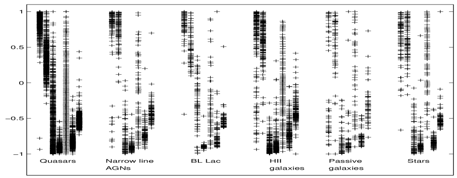
Figure 1: Normalized parameters $E$, $O-E$, log₁₀ $S_{p}$, $S_{i}/S_{p}$, radio-optical separation, PSF($E$) and PSF($O$), ordered from left to right, for each class.

An ANN is a computational tool which provides a non-linear parametrized mapping between a set of input parameters and one or more outputs. The type of ANN we used is the multi-layer perceptron (hereafter MLP; Bishop 1995; Bailer-Jones, Gupta & Singh 2001). A particular ANN architecture may be denoted as $N_{\rm in}:N_{1}:N_{2}:\ldots:N_{\rm out}$, where $N_{\rm in}$ is the number of input parameters, $N_{\rm 1}$ is the number of nodes in the first hidden layer and so forth, and $N_{\rm out}$ is the number of nodes in the output layer. The nodes are connected, each connection carrying a weight and each node carrying a bias. For our work we assume that every node is connected to every node in the previous layer and every node in the next layer only. Each node receives the output of all the nodes in the previous layer and produces its own output, which then feeds the nodes in the next layer. At a node in layer $s$ the following calculation is obtained

$$z=\sum_{j=1}^{m}x_{j}^{s-1}w_{jk}^{s}+b_{k},$$ (1)

where $x_{j}^{s-1}$ are the inputs from the previous layer (with $m$ nodes), and $w_{jk}$ and $b_{k}$ are respectively the weights and the bias of the node. Then the signal output of the node is $x_{k}^{s}=g(z)$, where $g$ is the non-linear activation or transfer function. In order to obtain the correct mapping, a set of representative input-output data is used for the training, a process in which the weights and biases are optimized to minimize the error in the outputs.

We used the same set of seven input parameters adopted by White et al. (2000), normalizing each of them to the range $[-1,1]$. In order to have homogeneous data sets we did not include the 28 candidates missed in APM $E$ or $O$ or both, and for which White et al. used the APS magnitudes (Minnesota Automated Plate Scanner POSS-I catalogue, Pennington et al. 1993). The number of FBQS-2 candidates with spectral classification and homogeneous data was reduced to 1112 for this reason. The distribution is as follows: 627 quasars, 94 narrow line AGNs, 67 BL Lac, 187 HII galaxies, 51 passive galaxies and 86 stars.

The network output consisted of a single node, with the target values set during the training as 1 for quasars and 0 for nonquasars. For the output node we used a logarithmic sigmoid activation function of the form $g(z)=1/[1+exp(-z)]$, in the range [0,1]. The actual output of the ANN is then an estimate of the probability that the source is a quasar, and it is denoted as $p$(Q) (Richard and Lippmann 1991). The transfer function for the hidden nodes was $g(z)=tanh(z)=2/[1+exp(-2z)]-1$, in the range $[-1,1]$.

Fig. 1 shows the normalized input parameters for the six classes. Although the covered parameter space varies between classes, there is a large degree of overlapping between quasars and nonquasars, which will certainly limit the performance of the classification. In fact, the category of nonquasars has an increased intrinsic scatter due to the presence of classes with different physical nature and covering different regions of the parameter space.

The error function we used was the mean of the squared errors, of the form

$$mse={1\over N}\sum_{i=1}^{N}(p_{i}-t_{i})^{2},$$ (2)

where $p_{i}$ and $t_{i}$ are, respectively, output (probability of being a quasar) and target value for the $i$th object. The sum of the squared errors has been widely used as the minimizing error function for classification with the MLP (Richard and Lippmann 1991, Bishop 1995, Lahav et al. 1996, Bailer-Jones et al. 2001, Ball et al. 2004). Although on theoretical grounds there are more appropriate error functions for classification, such as cross-entropy (which assumes the expected noise distribution for discrete variables), the sum-of-squares error has proven to yield the same performance as cross-entropy for MLP classification on real-world problems with large databases (Richard and Lippmann 1991). In addition, the sum-of-squares error has the advantage that the determination of the network parameters represents a linear optimization problem, in particular, the powerful Levenberg-Marquardt algorithm for parameter optimization is applicable specifically to a sum-of-squares error function (Bishop 1995). Based on these results, we used the $mse$ error function and applied the Levenberg-Marquardt algorithm, which is the default optimization technique used for batch-training (weights and biases updated after all the input vectors are presented to the network) in the Matlab Neural Network Toolbox. The Levenberg-Marquardt algorithm is the fastest method for training moderate-sized neural networks (Hagan & Menhaj 1994).

Regardless of the optimization algorithm employed, one of the main problems in the training process is that of “overfitting”, i.e. the ANN tends to memorize the outputs, instead of modelling the general intrinsic relationships in the data. In order to reduce this problem we used training with validation error. With this method, the training that is being carried out in the training set is automatically stopped when the error obtained running the trained network in another set, the validation set, does not decrease for a given number of iterations. We adopted for this parameter, known as maxfail in Matlab, a value of 20, instead of the default value of 5 iterations. An additional independent set, the test set, is needed to evaluate the ANN performance.

Following the procedure adopted by White et al., we divided the initial sample of candidates in four subsets or folds (they used five) of approximately similar sizes. Alike White et al., who selected the folds randomly, we chose them to have similar fractions of the different object types as the total sample. Setting aside each subset, the remaining three were used for the training and validation, and the subset itself was used for the test. The size of the test fold, of about 275 objects (i.e. 1/4 of the candidates), was selected to insure the inclusion of about a dozen of objects of the classes with fewer members, like passive galaxies and BL Lac. The three subsets used for training and validation were firstly combined and then randomly divided in two groups: one forming the training set, with 2/3 of the candidates, and the other forming the validation set, with the remaining 1/3, each of them with similar proportions of object types as the total sample. Repeating the procedure for each of the four folds, we obtained four different classifiers, with the advantage of having used all the objects for the training/validation and all the objects for the test, and therefore having optimized the statistics.

The ANN was run $10\times 10$ times per fold. The first factor accounts for the obliged repetition in an algorithm that includes randomization (for example in the seeds for the initial weights of the ANN) to avoid poor local minima. The second one arises from the use of 10 different splittings to separate the training and the validation sets. In order to choose the best ANN of the 100 runs, we first selected the splitting of the training and validation sets that gave the lowest value of the mean squared error, $\overline{mse}$, averaged over the 10 fits. Adopting $mse=0.5\times{mse}_{\rm train}+0.5\times{mse}_{\rm valid}$ for each run,

$$\overline{mse}=0.5\times\overline{mse}_{\rm train}+0.5\times\overline{mse}_{\rm valid}$$ (3)

We then checked if the relation

$$\overline{|{mse}_{\rm train}-{mse}_{\rm valid}|/{mse}_{\rm train}}<0.15$$ (4)

was satisfied for the splitting, to ensure that the errors in the validation and training were not only small, but also roughly similar (within 15% on average). In the case that this condition failed, the splitting with the next minimum value $\overline{mse}$ was checked for condition (4) and so forth. Once the splitting was selected we chose amongst the 10 ANNs the one with the minimum value of $mse=0.5\times{mse}_{\rm train}+0.5\times{mse}_{\rm valid}$ and satisfying

$$|{mse}_{\rm train}-{mse}_{\rm valid}|/{mse}_{\rm train}<0.15$$ (5)

For a few cases two or more fits had the same minimum, we took then the first fit in running order. In the end we had a final ANN for each of the four test sets. Running each ANN for its corresponding test set we were able to obtain the values $p$(Q) for the 1112 candidates.

3.2 Results

We used two different ANN architectures. The first one, denoted as 7:1, does not include hidden layers and it is also known as a logistic discrimination model. The second architecture includes a hidden layer with two nodes, and it is denoted as 7:2:1. As we shall see, the performance of the classifier does not improve with the inclusion of a hidden layer (increasing the free parameters of the ANN from 8 to 19), therefore more complex architectures were not explored. At the end of this subsection we present the quasar probabilities obtained from the fitted ANNs for the list of FBQS-2 candidates without optical spectroscopy.

3.2.1 Logistic discrimination model

Fig. 2 shows $mse_{\rm train}$ and $mse_{\rm valid}$ for the 400 networks run (100 networks per test set $\times$ 4 test sets). We recall that each group of 100 networks is divided in 10 blocks, each of them corresponding to a different splitting of the validation-training sets, and each block is made of 10 fits. Some of the networks or whole splittings (blocks) produce peaks in $mse_{\rm train}$, in $mse_{\rm valid}$ or in both. The splittings showing peaks tend to have a higher $\overline{mse}$ than the splittings lacking thereof, therefore our choice of the minimum $\overline{mse}$ to select the best splitting. For 54% of the networks the validation set stopped the training. The number of iterations for the cases of validation stop is very small (below 12), with an average of $\sim$ 4 compared to the average $\sim$ 23 found for the networks stopped because of other reasons.

Figure 2: $mse_{\rm train}$ (continuous line) and $mse_{\rm valid}$ (dotted line) for the 400 ANNs run. The vertical lines mark the best ANN for each of the test sets.

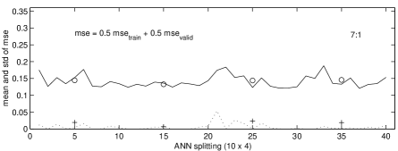
Figure 3: Mean (continuous line) and standard deviation (dotted line) of $mse$ ( $=0.5\times mse_{\rm train}+0.5\times mse_{\rm valid}$) over the 10 runs with similar test, training and validation sets. The first parameter is denoted as $\overline{mse}$ in the text. The meaning of the circles and crosses is explained in the text.

Fig. 3 shows $\overline{mse}$ and the standard deviation of $mse$ over the ten runs for each of the 40 different splittings (10 splittings per test set $\times$ 4 test sets). The scatter ranges from 0 to about 0.05, with an average for the 40 splittings of 0.006. The influence of the initial values on the performance of the selected network is negligible, since the standard deviation of $mse$ due to different initiations is clearly much lower than the mean values. The same occurs for the separation of the training and validation sets; the circles in Fig. 2 show the average of $\overline{mse}$ over the 10 different splittings per test set, and the averages are significantly larger than their standard deviations, symbolized as crosses. Finally, the figure also shows that the four mean values (one per test set) are very similar, with the standard deviation being much lower than the average (this average and standard deviation are not shown in the figure). The last result demonstrates that the performance of the network does not depend strongly on the particular selected test set either. The 4 best ANNs (one per test set) are marked with vertical lines in Fig. 2 and Table 1 summarizes some of their parameters.

Table 1: Parameters of the 4 selected ANNs for the logistic model

$mse_{\rm train}$	$mse_{\rm valid}$	$N_{\rm iter}$	$mse_{\rm test}$	$\overline{E}$
0.128	0.122	3 *	0.119	0.49
0.118	0.130	18	0.133	0.54
0.119	0.124	23	0.154	0.63
0.129	0.112	11 *	0.122	0.49

* : The results on the validation set stopped the training.

So far we have discussed the mean squared errors obtained in the training process. Column four of Table 1 gives the mean squared errors obtained for the test sets. The latter mse values generally show a good agreement with those obtained for the training and validation sets. However, a more interesting parameter for the purpose of assessing the performance of the network is the normalized error function (Bishop 1995), of the form

$$\overline{E}=\sum_{i=1}^{N}(p_{i}-t_{i})^{2}/\sum_{i=1}^{N}(\overline{t}-t_{i})^{2},$$ (6)

where $\overline{t}$ is the mean of the target data over the test set. This error function equals unity when the model is as good a predictor of the target data as the simple model $p=\overline{t}$, and equals zero if the model predicts the data values exactly. The value we found is around 0.55. Although the model is not good enough for classification, the results are powerful for our aim of selecting the best candidates. In fact, compared to the model that takes $p=\overline{t}$, which would give $mse_{\rm test}\sim 0.246$, the $mse$ obtained with the ANNs is reduced about a factor two. In the next paragraphs we present the results of the model in terms of completeness and efficiency of the subsamples of the best candidates that can be drawn from the ANN model.

Fig. 4 shows the distribution of $p$(Q) for the 1112 candidates and the logistic discrimination ANN. The model gives probabilities above 0.5 for most of the quasars, although there is a large number of them with probabilities below this value. Narrow line AGNs, HII galaxies, passive galaxies and stars tend to give low probabilities, and the model provides therefore a good means to reject objects of these types. The number of BL Lac objects is small, and their distribution of $p$(Q) is rather flat, and even slightly increased at high probabilities, therefore the current model is not able to reject these sources. The last problem was also found by White et al. using the decision tree classifier.

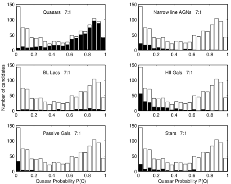
Figure 4: Distribution of $p$(Q) for the logistic discrimination model. The shaded distributions correspond to the objects of the indicated types (quasars, narrow line AGNs, BL Lacs, etc).

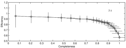
Figure 5: Efficiency vs. completeness of the sample for $p$(Q) $>0,0.05,0.1,0.15,0.2,\ldots 0.95$ (right to left) and the logistic model. Poissonian errors were assumed.

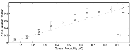
Figure 6: Fraction of candidates that are quasars as a function of $p$(Q) for the logistic model. Poissonian errors were assumed.

The efficiency and completeness of the sample as a function of the quasar probability threshold $p_{C}$(Q) are shown in Fig. 5. The logistic model allows to obtain a high reliability at a high completeness: for completenesses of 70, 80 and 90% the corresponding reliabilities are 90, 87 and 81%. Fig. 6 shows the fraction of candidates that are quasars as a function of $p$(Q). The fraction is slightly above $p$(Q) (about 0.1 in the range from $p$(Q) 0.3 to 0.8), i.e. the likelihood that a candidate turns out to be a quasar is slightly larger than the probability given by the model.

Fig. 4 shows that the majority of the high-$p$(Q) candidates that are not quasars are BL Lac objects. Taking $p$(Q)$>$0.75 there are 353 quasars, 24 BL Lacs, two narrow line AGNs, three HII galaxies, a passive galaxy and three stars. An inspection of the input parameters for the nonquasars revealed as the most outstanding result that the whole population of BL Lacs has radio fluxes higher than those found for the remaining nonquasar classes, and similar to those typically found in quasars (see Fig. 7a). About 36% of the BL Lac have $p$(Q)$>$0.75 and Figs. 7b and 7c show that these correspond to the cases with bluer $O-E$ colours. The efficiency of quasar selection using the cut at $p$(Q)$=$0.75 is 91% (353/386) and increases to 98% considering quasar or BL Lac selection (377/386). The corresponding completeness would be 56% (353/627) for quasars and 54% (377/694) for quasars or BL Lac. The completeness decreases in the latter case since only blue BL Lac are confused with quasars.

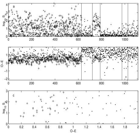
Figure 7: a and b: Log₁₀$(S_{p})$ and $O-E$ for the classes of quasars, narrow line AGNs, BL Lac, HII galaxies, passive galaxies and stars (separated by vertical lines). c: Log₁₀$(S_{p})$ versus $O-E$ for the BL Lac. Crosses correspond to $p$(Q)$>$0.75 for the 7:1 model.

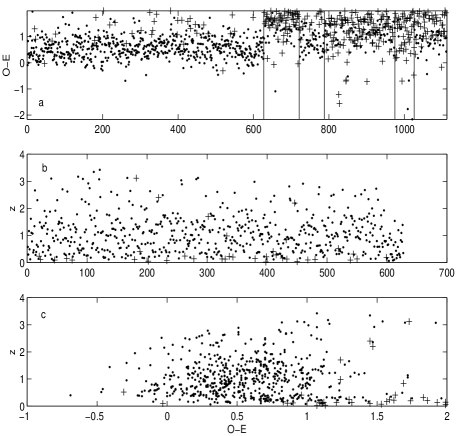
Figure 8: a: $O-E$ for the classes of quasars, narrow line AGNs, BL Lac, HII galaxies, passive galaxies and stars (separated by vertical lines). b and c: $z$ and $z$ versus $O-E$ for the quasars. Crosses correspond to $p$(Q)$<$0.2 for the 7:1 model.

At the other extreme, there are 36 quasars with probabilities $p$(Q)$<$0.2, and their most significant differences with respect to the remaining quasars are their redder $O-E$ colours and lower redshifts, with twenty-five of them at $z<0.25$ (see Figs. 8a, 8b, 8c). The misclassified quasars also differ, although to a lower extent, in their larger integrated-to-peak radio flux ratio, larger optical-radio separation and wider PSF. The low probabilities found for the low-$z$ quasars should not be regarded as a limitation of the classifier, since at low redshifts the host galaxy is expected to be slightly resolved and to have a noticeable contribution to the total ”galaxy + quasar” emission. This contribution, imperceptible at higher redshifts, is the most likely explanation for the differences in the input parameters between low-$z$ quasars and the remaining quasars.

If only the quasars with $z\geq 0.25$ are considered, the fraction of them with $p$(Q)$<$0.2 drops from 6% (36/627) to 2% (11/558). As for the probability cut $p$(Q)$>$0.75, the efficiency remains at 91% and the completeness increases from 56% to 62%. White et al. also found, using the decision tree classifier, that the great majority of quasars with low probabilities were at low redshift (out of 30 quasars with $p(Q)<0.2$, 24 had $z<0.25$).

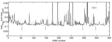
Figure 9: Similar to Fig. 1, but for the 7:2:1 architecture.

Figure 10: Similar to Fig. 2, but for the 7:2:1 architecture.

3.2.2 ANN with a hidden layer

In this subsection we present the results for the ANN model 7:2:1. Fig. 9 shows $mse_{\rm train}$ and $mse_{\rm valid}$ for the 400 networks. Three main differences with respect to the model without a hidden layer are revealed: (i) the distribution of $mse_{\rm train}$ is more noisy but there is a better agreement between $mse_{\rm train}$ and $mse_{\rm valid}$, (ii) validation stopping dominates (96% of the cases) over the remaining reasons to stop the training and (iii) the number of iterations for the cases of validation stopping reaches higher values, with an average $\sim$ 33 iterations. Fig. 10 shows the average and standard deviation of $mse$ over the ten runs for each of the 10 splittings and for each of the 4 test sets. The large variations of $mse$ are clearly evident from this figure: the standard deviation of $mse$ ranges from 0.002 to 0.12, with an average for the 40 splittings of 0.027, i.e. 4.5 times larger than for the 7:1 architecture. However, for most of the training-validation-test configurations the scatter of $mse$ is still much lower than the mean value. Considering the averages per test set, the mean values for $\overline{mse}$ are also significantly larger than their standard deviations (denoted with circles and crosses respectively) and the same occurs considering the average over the four test sets. As occurred for the 7:1 model, the performance of the selected network does not depend strongly on changes of the initiation values, splitting for training-validation or choice of test set.

Table 2: Parameters of the 4 selected ANNs for the model 7:2:1

$mse_{\rm train}$	$mse_{\rm valid}$	$N_{\rm iter}$	$mse_{\rm test}$	$\overline{E}$
0.112	0.126	14 *	0.110	0.45
0.119	0.121	8	0.127	0.52
0.109	0.118	16 *	0.146	0.60
0.114	0.106	27 *	0.127	0.51

The relevant parameters of the 4 selected ANNs are summarized in Table 2. The $mse$ values for the test sets generally show a good agreement with the values obtained for the train and validation sets. Both $mse_{\rm test}$ and the normalized error function $\overline{E}$ are on average similar to those obtained for the 7:1 architecture.

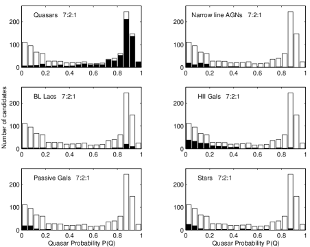
Figure 11: Similar to Fig. 3, but for the 7:2:1 architecture.

Fig. 11 shows the distribution of $p$(Q) for the 1112 candidates and the 7:2:1 model. The distribution is more peaked towards the extreme values of the probabilities than in the logistic model. In this respect, the 7:2:1 model gives a better agreement with the results from OC1 than the logistic model. As occurred for the logistic model and OC1, all the nonquasar classes except for the BL Lac tend to give low probabilities.

The efficiency and completeness of the sample as a function of the quasar probability threshold are very similar to the values found for the logistic model. For completenesses of 70, 80 and 90% the corresponding reliabilities are 88, 87 and 81% respectively. Again there is a very good agreement between $p$(Q) and the likelihood that a candidate with $p$(Q) turns out to be a quasar (measured by the fraction of candidates at this $p$(Q) that are quasars), except for $p$(Q) around 0.55, where the likelihood is increased by an amount around 0.1.

Table 3: Efficiency and completeness of quasar selection from the sample of FBQS-2 candidates using ANNs

Size of spectroscopically identified sample 1112
Training+validation set size $\sim$ 840
Total number of quasars  627
ANN 7:1				ANN 7:2:1
Completeness/Efficiency   70% / 90%				Completeness/Efficiency   70% / 88%
80% / 87%				80% / 87%
90% / 81%				90% / 81%
$p$(Q)$<$0.2	Quasars	36		$p$(Q)$<$0.2	Quasars	39
$p$(Q)$>$0.75	Candidates	386		$p$(Q)$>$0.85	Candidates	418
	Quasars	353			Quasars	372
	BL Lac	24			BL Lac	30
	Efficiency for quasars	91%			Efficiency for quasars	89%
	Efficiency for quasars + BL Lac	98%			Efficiency for quasars + BL Lac	96%
	Completeness for quasars	56%			Completeness for quasars	59%
	Completeness for quasars + BL Lac	54%			Completeness for quasars + BL Lac	58%

Taking $p_{C}$(Q)=0.85, there are 372 quasars, 30 BL Lacs, 3 narrow line AGNs, five HII galaxies and eight stars above this cut. A result similar to the one obtained in Fig. 7 for the logistic model is found for the 7:2:1 architecture: the majority of the high-$p$(Q) nonquasars are blue BL Lac objects. The efficiency of quasar selection for this threshold is 89% and increases to 96% considering quasar or BL Lac selection. The corresponding completeness would be 59% for quasars and 58% for quasars or BL Lac.

Regarding the limit of low probabilities we find thirty-nine quasars with $p$(Q)$<$0.2, twenty-two of them with redshifts below 0.25. We find similar results to those presented in Fig. 8 for the logistic model: most of the misclassified quasars have lower redshifts and redder $O-E$ colours than the remaining quasars, as well as higher integrated-to-peak radio flux ratios and wider PSFs, and these results are indicative of an appreciable contribution of the emission from the host galaxy. If only the quasars with $z\geq 0.25$ are considered, the fraction of them with $p$(Q)$<$0.2 decreases from 6% to 3%. As for the probability cut $p$(Q)$>$0.85, the efficiency would remain at 89% and the completeness would increase from 59% to 65%.

Table 3 presents a summary of the performance of the two ANN models. Both use similar training set sizes and achieve similar efficiencies for completeness in the range from 70 to 90%. The main difference is that the distribution of $p$(Q) is more peaked towards the extreme values (0 and 1) for the model with a hidden layer than for the logistic one.

Fig. 12 shows that the distribution of efficiency versus completeness for the two ANN models and the oblique decision tree OC1 are very similar. The agreement obtained for the three different classifiers favours the interpretation that the found accuracy - $\sim$ 87% at 80% completeness - is more limited by the data structure itself (i.e. the large degree of overlapping between quasars and nonquasars in the input parameter space) than by the complexity of the algorithms. The ANN and the decision tree classifiers both point to BL Lac (blue BL Lac for ANNs) and low-$z$ quasars as the object types that most severely limit the accuracy of quasar selection, the former producing intruders (false alarms), and the latter misclassifications.

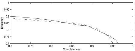
Figure 12: Efficiency versus completeness for the 7:1 ANN (continuous line), the 7:2:1 ANN (dotted line) and the OC1 decision tree (dash-dotted line).

Owens et al. (1996) apply the decision tree OC1 for the morphological classification of galaxies taken from the ESO-LV catalogue (Lauberts & Valentijn 1989), and present a comparison of their results with those obtained by Storrie-Lombardi et al. (1992) for the same sample using ANNs. The classification into six classes has an overall efficiency around 63% for the two methods, with a difference between them lower than 3%. Owens et al. (1996) attribute the found similarity to limitations in the classification accuracy intrinsic to the database (errors in the assumed classification for some of the galaxies and a poorly defined separation between classes). Our work and Owens et al. (1996) show examples of classification from astronomical databases in which OC1 and ANNs give similar performances, probably at the limit set by the database itself, whose attributes do not provide enough information for a more accurate classification.

3.2.3 Predictions for the FBQS-2 candidates without spectroscopic classification

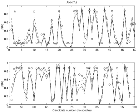
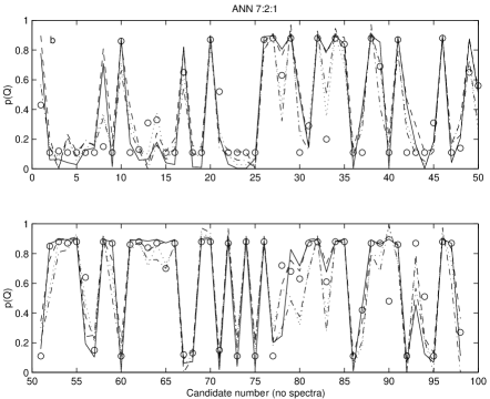
Figure 13: $p$(Q) distribution for the 98 FBQS-2 candidates without spectroscopic classification in White et al. (2000) using the ANN architectures 7:1 (a) and 7:2:1 (b). The four line types correspond to the four selected ANNs. Circles correspond to the $p$(Q) values obtained by White et al. with OC1.

The ANN models 7:1 and 7:2:1 were used to estimate the probabilities $p$(Q) for the 98 FBQS-2 candidates without spectral classification in White et al. We adopted four classifiers per model, corresponding to the four selected ANNs (parameters described in Tables 1 and 2). Fig. 13a shows the probabilities obtained with the 7:1 model - plotted with a different line type for each ANN - and using OC1 (White et al.). There is a good agreement between the probabilities predicted with the four ANNs and between them and the values from OC1. Similar results are found for the 7:2:1 model (Fig. 13b). The probabilities obtained for the ANN models and OC1 are listed in Table 4. For the ANN models we give the mean and standard deviation of $p$(Q) over the four selected ANNs.

Table 4: Quasar probabilities for the 98 candidates without spectroscopic classification in White et al. (2000)

Name	ANN 7:1		ANN7:2:1		OC1		Name	ANN 7:1		ANN 7:2:1		OC1
FBQS J	$\overline{p}$(Q)	$\sigma$	$\overline{p}$(Q)	$\sigma$	$p$(Q)		FBQS J	$\overline{p}$(Q)	$\sigma$	$\overline{p}$(Q)	$\sigma$	$p$(Q)
071505.4+340501	0.61	0.08	0.70	0.17	0.43		122251.3+331640	0.25	0.07	0.39	0.15	0.56
071650.6+350520	0.15	0.04	0.14	0.06	0.11		122407.3+375332	0.30	0.07	0.26	0.08	0.11
071903.2+342550	0.03	0.01	0.04	0.04	0.12		122520.4+292420	0.55	0.09	0.67	0.17	0.85
073018.1+224502	0.17	0.07	0.17	0.09	0.11		122856.6+355635	0.85	0.07	0.87	0.04	0.88
073237.9+342952	0.06	0.02	0.07	0.04	0.11		123659.5+423641	0.85	0.04	0.87	0.03	0.87
073317.3+223725	0.12	0.06	0.16	0.03	0.11		123757.9+223430	0.94	0.03	0.91	0.02	0.88
073833.5+360957	0.18	0.07	0.16	0.02	0.11		124327.8+232811	0.36	0.06	0.32	0.13	0.64
074342.2+321543	0.40	0.08	0.56	0.24	0.15		124444.5+223305	0.20	0.10	0.19	0.06	0.15
082711.2+223323	0.10	0.02	0.12	0.08	0.11		124840.4+241240	0.84	0.05	0.90	0.02	0.88
083522.7+424258	0.63	0.09	0.78	0.10	0.86		124958.8+245233	0.62	0.07	0.70	0.16	0.87
085552.7+384325	0.31	0.08	0.29	0.10	0.11		125018.1+364914	0.10	0.02	0.11	0.07	0.11
085624.8+345024	0.12	0.04	0.12	0.04	0.13		125142.2+240435	0.77	0.07	0.86	0.03	0.86
091309.2+413635	0.09	0.03	0.05	0.04	0.31		125256.9+252503	0.82	0.06	0.88	0.01	0.88
091833.8+315620	0.30	0.06	0.24	0.10	0.33		125444.7+425305	0.63	0.10	0.79	0.07	0.84
091845.7+233833	0.02	0.00	0.07	0.04	0.11		131823.4+262623	0.84	0.06	0.84	0.06	0.87
093456.7+263054	0.15	0.03	0.14	0.08	0.11		131848.3+252815	0.70	0.09	0.80	0.09	0.70
101355.2+300546	0.59	0.07	0.71	0.13	0.65		132324.1+251809	0.84	0.05	0.87	0.02	0.87
102802.9+304743	0.08	0.02	0.09	0.06	0.11		134531.0+255504	0.05	0.00	0.05	0.04	0.12
102857.6+344054	0.07	0.01	0.08	0.06	0.11		134540.0+280123	0.13	0.02	0.11	0.03	0.13
103346.3+233220	0.81	0.05	0.88	0.03	0.87		140819.3+294950	0.95	0.02	0.93	0.03	0.88
103818.1+424442	0.28	0.05	0.20	0.05	0.52		141257.7+232618	0.92	0.04	0.91	0.02	0.88
105330.9+331342	0.07	0.02	0.09	0.04	0.11		143655.7+234928	0.03	0.00	0.06	0.04	0.15
105653.3+331945	0.00	0.00	0.05	0.05	0.11		144053.9+270642	0.94	0.04	0.93	0.03	0.87
110113.8+323155	0.00	0.00	0.05	0.05	0.11		144755.7+382813	0.19	0.05	0.16	0.08	0.11
112242.8+414355	0.04	0.01	0.04	0.04	0.11		145007.2+315050	0.90	0.05	0.91	0.01	0.88
113020.4+422204	0.76	0.07	0.84	0.04	0.87		150228.5+354455	0.13	0.05	0.14	0.08	0.11
113124.2+261951	0.87	0.05	0.90	0.01	0.88		150428.0+262419	0.81	0.07	0.88	0.03	0.88
113324.7+323449	0.45	0.05	0.58	0.24	0.63		150435.8+335728	0.27	0.08	0.22	0.05	0.11
113442.0+411330	0.96	0.02	0.93	0.04	0.88		150555.4+424415	0.48	0.09	0.43	0.18	0.72
113609.0+360641	0.26	0.06	0.37	0.16	0.11		151314.9+342111	0.47	0.08	0.64	0.17	0.68
113639.1+372651	0.19	0.03	0.18	0.07	0.29		151627.3+305220	0.34	0.09	0.52	0.21	0.63
113707.7+290324	0.92	0.03	0.91	0.01	0.88		151913.4+252134	0.71	0.10	0.79	0.11	0.87
113921.2+350748	0.37	0.10	0.61	0.21	0.20		152049.1+375219	0.85	0.06	0.90	0.02	0.88
114048.0+332908	0.91	0.03	0.91	0.02	0.88		152158.4+381814	0.39	0.08	0.52	0.22	0.61
114111.1+300442	0.65	0.08	0.80	0.08	0.84		152547.2+425210	0.87	0.05	0.88	0.00	0.88
115244.4+311123	0.06	0.01	0.08	0.06	0.11		153402.2+425249	0.87	0.04	0.88	0.01	0.88
115943.8+303348	0.28	0.07	0.33	0.06	0.11		153411.3+262124	0.01	0.00	0.06	0.05	0.11
120354.7+371137	0.95	0.03	0.93	0.03	0.88		153420.2+413007	0.19	0.06	0.29	0.12	0.42
120908.4+265131	0.57	0.09	0.67	0.18	0.69		153521.6+331826	0.76	0.07	0.83	0.05	0.87
121147.1+240736	0.13	0.03	0.13	0.08	0.11		153818.6+410548	0.73	0.07	0.80	0.09	0.87
121232.3+425821	0.76	0.06	0.83	0.06	0.87		154007.6+252836	0.99	0.01	0.95	0.05	0.48
121355.3+365255	0.26	0.05	0.36	0.11	0.11		154049.2+390351	0.67	0.08	0.80	0.07	0.86
121529.6+391200	0.14	0.03	0.17	0.08	0.11		155537.5+221327	0.06	0.02	0.04	0.04	0.11
121727.8+290449	0.02	0.01	0.05	0.05	0.11		155723.9+420825	0.67	0.09	0.64	0.16	0.87
121902.5+222416	0.18	0.06	0.15	0.03	0.31		160531.1+243147	0.22	0.09	0.20	0.05	0.51
122004.3+311148	0.89	0.04	0.89	0.01	0.88		162237.8+235943	0.05	0.02	0.07	0.05	0.11
122034.6+363357	0.12	0.06	0.13	0.06	0.11		163718.8+272607	0.96	0.02	0.93	0.03	0.88
122208.1+240012	0.33	0.08	0.27	0.06	0.14		164733.9+364055	0.69	0.09	0.76	0.12	0.87
122221.3+372335	0.66	0.06	0.80	0.09	0.65		170753.9+272418	0.18	0.04	0.18	0.16	0.27

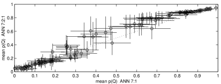
Figure 14: Comparison between $\overline{p}$(Q) for the 7:1 and the 7:2:1 ANNs, for the FBQS-2 candidates without spectroscopic classification in White et al. (2000).

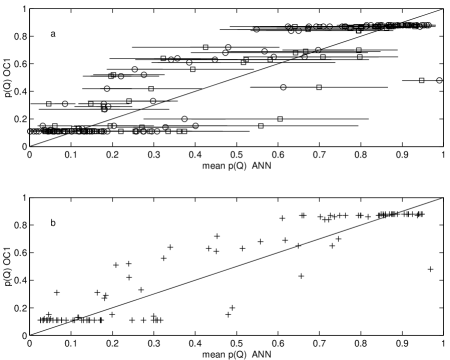
Figure 15: a: $p$(Q) OC1 versus $\overline{p}$(Q) for the 7:1 (circles) and 7:2:1 (squares) ANN models. b: $p$(Q) OC1 versus the average of $\overline{p}$(Q) for the 7:1 and the 7:2:1 ANN models.

Fig. 14 shows $\overline{p}$(Q) for the 7:2:1 model versus $\overline{p}$(Q) for the 7:1 model. The agreement between the two predictions is generally very good, with the largest discrepancies occurring at intermediate probabilities, where the candidates’ parameters do not fit the quasar class nor the nonquasar class. The average difference between $\overline{p}$(Q) for the two models (7:2:1 $-$ 7:1) is of only 0.04, and the standard deviation of the difference is 0.06.

Fig. 15a shows $p$(Q) for OC1 versus $\overline{p}$(Q) for the two ANN models. Fig. 15b is a similar plot in which the abcissa corresponds to the average of $\overline{p}$(Q) for the two ANN models. The mean and standard deviation of the differences are (0.04, 0.14) for OC1$-$7:1, (0.005, 0.13) for OC1$-$7:2:1 and (0.02, 0.13) for OC1 minus the average of the two ANN models. Figs. 14 and 15, and the standard deviation values, show that the agreement in $\overline{p}$(Q) between the two ANN models is better than the agreement between any of them (or their average) and OC1.

The 98 sources in Table 4 were sought for associations in the NASA Extragalactic Database (NED). Five of them are confirmed extragalactic sources with spectroscopic redshift. FBQS J091309.2+413635 and FBQS J125018.1+364914 are classified as Ultraluminous Infrared Galaxies with redshifts 0.22 and 0.279 in Stanford, Stern & de Breuck (2000). The authors state that the majority of the ULIRGs in their sample are star forming galaxies, and this interpretation is consistent with the low quasar probability we found, of $\sim$ 0.07 and $\sim$ 0.105 respectively (0.31 and 0.11 with OC1). FBQS J120354.7+371137, with $z=0.401$, has broad emission lines (Appenzeller et al. 1998), therefore corresponds to the quasar classification in our study, and it has in fact a quasar probability $\sim$ 0.94 (0.88 for OC1). A similar case is FBQS J125142.2+240435, with $z=0.188$ and broad emission lines (Chen et al. 2002), and also a high quasar probability, $\sim$ 0.82 (0.86 for OC1). FBQS J153411.3+262124 has $z=0.1294$ and spectral type “possibly Seyfert” (Keel, de Grijp & Miley 1988). We measure for the source $p$(Q) $\sim$ 0.04 (OC1 gives 0.11), which favours a spectral type Seyfert2, of narrow emission lines. In addition, four objects in Table 4 have spectroscopic classification in the recent Sloan Digital Sky Survey Data Release 2 (SDSS DR2). FBQS J083522.7+424258, FBQS J153402.2+425249 and FBQS J164733.9+364055 are quasars at $z=0.805$, $z=0.649$ and $z=1.566$, with $p$(Q) $\sim$ 0.71, $\sim$ 0.88 and $\sim$ 0.73 (0.86, 0.88 and 0.87 with OC1). FBQS J074342.2+321543 is a star with $p$(Q) $\sim$ 0.48 (0.15 for OC1). Summarizing these results, the inspection of NED and SDSS DR2 shows that the five FBQS candidates classified as quasars have in fact rather high quasar probabilities - $\sim$ 0.94, $\sim$ 0.82, $\sim$ 0.71, $\sim$ 0.88 and $\sim$ 0.73 -, whereas the two ULIRGs and the star have $p$(Q) values $\sim$ 0.07, $\sim$ 0.105 and $\sim$ 0.48, reinforcing the high efficiency of the ANN models.

4 Conclusions

In this work we analyse the performance of neural networks for the selection of quasar candidates from combined radio and optical surveys with photometric and morphological data. Our work is based on the candidate list leading to FBQS-2 (White et al. 2000), and the input parameters used are radio flux, integrated to peak flux ratio, photometry and point spread function in the red and blue bands, and radio-optical position separation.

Two ANN architectures were investigated: a logistic model (7:1) and a model with a hidden layer with two nodes (7:2:1), and both yielded similarly good performances, allowing to obtain subsamples of quasar candidates from FBQS-2 with efficiencies as large as 87% at 80% completeness. For comparison the quasar fraction from the original candidate list was 56%. More complex architectures were not explored, since the inclusion of the hidden layer - increasing the free parameters from 8 to 19 - did not improve the performance of the network. The efficiencies we find for completeness in the range 70 to 90% are 90–80%, similar to those found by White et al. using the oblique decision tree classifier OC1 and a similar sample size for the training. The lack of a clean separation between quasars and nonquasars in the parameter space certainly limits the accuracy of the classification, and the agreement in the performances obtained favours in fact the interpretation that the three classifiers approach the maximum value achievable with this database. Although none of the two artificial intelligence tools provides a secure quasar classification (say efficiency larger than 95% for a reasonable completeness), they are powerful to prioritize targets for observation.

We report the probabilities obtained with the two ANN models for the 98 FBQS-2 candidates without spectroscopic classification in White et al. Our results are compared with those found by White et al. using OC1. The three models are found to be in agreement, with a better match between the two ANN models (standard deviation of the difference in probabilities $\sim$ 0.06) than between them and OC1 (standard deviation $\sim$ 0.13).

To our knowledge, this is the first work exploring the performance of ANNs for the selection of quasar samples. Our study demonstrates the ability of ANNs for automated classification in astronomical databases.

References

- [1] Appenzeller I. et al., 1998, ApJS 117, 319
- [2] Bailer-Jones C.A.L., Irwin M., von Hippel T., 1998, MNRAS, 298, 361
- [3] Bailer-Jones C.A.L., Gupta R., Singh H.P., 2001, in Gupta R., Singh H.P., Bailer-Jones C.A.L., eds, Automated Data Analysis in Astronomy, Narosa Publishing House, New Delhi, India, p. 51
- [4] Ball, N.M., Loveday J., Fukugita M., Nakamura O., Okamura S., Brinkmann J., Brunner R.J., 2004, MNRAS, 348, 1038
- [5] Bishop C.M., 1995, Neural Networks for Pattern Recognition, Oxford University Press
- [6] Bertin E., Arnouts S., 1996, A&AS, 117, 393
- [7] Chen Y., He X.-T., Wu J.-W., Li Q.-K., Green R.F., Voges W., 2002, AJ, 123, 578
- [8] Firth A.E., Lahav O., Somerville R.S., 2003, MNRAS, 339, 1195
- [9] Folkes S.R., Lahav O., Maddox S.J., 1996, MNRAS, 283, 651
- [10] Hagan M. T., Menhaj M., 1994, IEEE Transactions on Neural Networks, vol. 5, no. 6, 989
- [11] Keel W.C., de Grijp M.H.K., Miley G.K., 1988, A&A, 203, 250
- [12] Lahav O., Naim A., Sodré L. Jr, Storrie-Lombardi M.C., 1996, MNRAS, 283, 207
- [13] Lauberts A., Valentijn E.A., 1989, The Surface Photometry Catalogue of the ESO-Uppsala Galaxies. European Southern Observatory, Munich
- [14] McMahon R.G., Irwin M.J., 1992, in MacGillivray H.T., Thomson E.B., eds, Digitised Optical Sky Surveys. Dordrecht:Kluwer, p. 417
- [15] Murthy S.K., Kasif S., Salzberg S., 1994, J. Artif. Intell. Res., 2, 1
- [16] Owens E.A., Griffiths R.E., Ratnatunga K.U., 1996, MNRAS, 281, 153
- [17] Pennington R.L., Humphreys R.M., Odewahn S.D., Zumach W., Thurmes P.M., 1993, PASP, 107, 279
- [18] Richard M.D., Lippmann, R.P., 1991, Neural Computation 3, 461
- [19] Stanford S.A., Stern D., de Breuck C., ApJS, 131, 185
- [20] Storrie-Lombardi M.C., Lahav O., Sodré L. Jr., Storrie-Lombardi L.J., 1992, MNRAS, 259, 8p
- [21] Tagliaferri R. et al., 2003, Neural networks in Astronomy. Neural Networks 16, 297
- [22] White R.L. et al., 2000, ApJSS, 126, 133