Large scale systematic signals in weak lensing surveys

Abstract

We use numerical simulations to model the effect of seeing and extinction modulations on weak lensing surveys. We find that systematic fluctuations in the shear amplitude and source depth can give rise to changes in the $E$-mode signal and to varying amplitudes of large scale $B$-modes. Exquisite control of such systematics will be required as we approach the era of precision cosmology with weak lensing.

1. Introduction

Weak gravitational lensing of distant galaxies by foreground large scale structure has emerged as a powerful tool for modern cosmology (see Mellier, 1999; Bartelmann & Schneider, 2001; Refregier, 2003a, for reviews), which has already provided constraints on cosmological parameters (see e.g. Hoekstra, Yee, & Gladders, 2002; van Waerbeke & Mellier, 2003, for the current status) and been touted for its potential to constrain dark energy (Benabed & Bernardeau, 2001; Huterer, 2002; Hu, 2002; Abazajian & Dodelson, 2003; Benabed & van Waerbeke, 2003; Jain & Taylor, 2003; Heavens, 2003; Refregier, 2003b; Takada & Jain, 2003; Bernstein & Jain, 2004; Takada & White, 2004).

The technique relies upon the measurement of the distortion that lensing induces in the shapes of galaxy images. The percent level distortion induced by large-scale structure is generally referred to as cosmic shear. As the power of cosmic shear surveys increases, requirements that systematic errors in the measurement of these images be accurately accounted for has become increasingly stringent. Fortunately nature has provided us with a means to test for some of these systematic errors. Since lensing arises from a scalar gravitational potential, the shear pattern it generates has a particular form. For example, the shear pattern around an isolated, spherically symmetric mass distribution is tangential. Since this pattern has even parity it is often referred to as a (positive) $E$-mode. In the absence of lens-lens coupling or higher order effects the shear pattern induced by lensing is pure $E$. A $45^{\circ}$ rotation of the shear, to produce the (parity-odd) $B$-mode, will null such a signal. Thus, a simple diagnostic test for a wide range of systematic errors is the presence of a $B$-mode in the lensing maps.

In this paper, we model the effect of systematic errors in the seeing correction and extinction on simulated weak lensing maps. We show that fluctuations in amplitude and depth of the signal across a field can generate $B$-mode signals on large angular scales. However these $B$-modes do not closely track the change in the $E$-mode power, and thus cannot be used to correct for these systematic errors.

We begin with a brief description of these effects in §2, and then describe how we generate simulated weak lensing maps in §3. We discuss how we model the effects of seeing and dust extinction in the source population in §4, and present our results in §5 before concluding in §6.

2. Seeing and Extinction

One systematic effect that has received particular attention is the correction for the point spread function (PSF) (e.g. Kaiser et al., 1995; Hoekstra et al., 1998; Kuijken, 1999; Kaiser, 2000; Bernstein & Jarvis, 2002; Hirata & Seljak, 2003; Hoekstra, 2004) and its anisotropy. Here, we consider two related issues that might prove troublesome: the effects of fluctuations in seeing conditions and of galactic extinction.

Seeing causes a degradation in the lensing signal amplitude by circularizing the images of background galaxies. Corrections for this “isotropic” PSF effect have been studied using simulated images (e.g. Bacon et al., 2001; Erben et al., 2001) and by marginalizing over the uncertain shear calibration using a model fit to the power spectrum (Ishak et al., 2004). In practice a cosmic shear survey consists of many pointings of a telescope, and seeing can easily vary by a factor of two between the best and worst pointings; even chip to chip variations in the detector can yield corrective factors that differ by as much as 10%. Systematic errors in the lensing measurement may therefore be introduced on the scale of the telescope pointings or of individual chips in the detectors due to imperfections in this correction.

A second effect of seeing fluctuations is to modulate the effective depth of the survey by down weighting smaller images which have become too circularized. This not only reduces the signal to noise, it also alters the source redshift distribution, and can therefore be expected to have an effect that resembles source redshift clustering (e.g. Bernardeau, 1998), although on a different angular scale. The measured signal will then probe structures at different depths in different regions of the sky. Variable galactic extinction in a magnitude limited survey will have a similar effect, although it should not be correlated with the lensing signal.

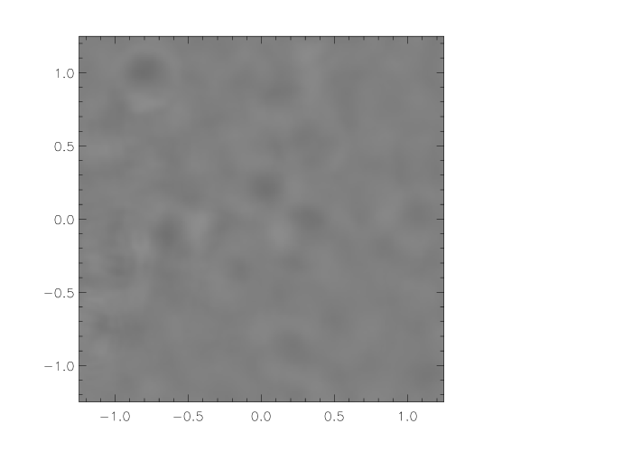
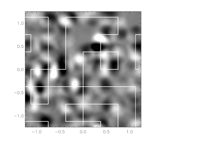
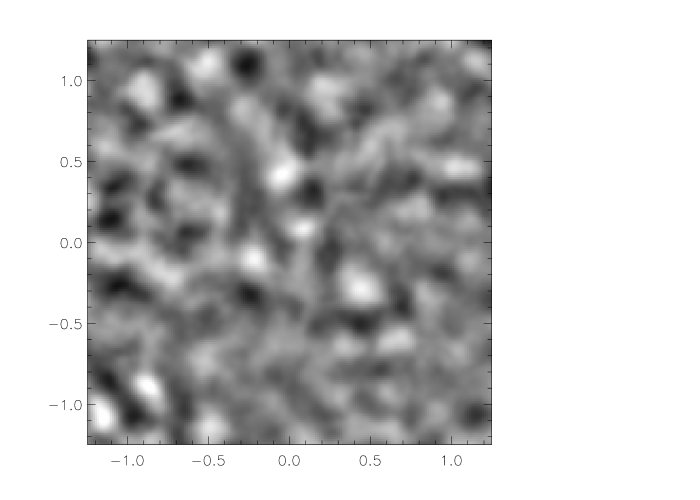
Figure 1.— $B$-mode aperture mass on a $15^{\prime}$ scale, for $2.5^{\circ}\times 2.5^{\circ}$ fields. The left panel is with no modulation, the center panel includes sharp, 10%, modulations in the seeing correction on a $22^{\prime}$ scale (as detailed in the text and outlined by the solid lines), and the right panel is for 10% modulations in the source redshift relation at a scale of $8^{\prime}$. The greyscale is linear and spans $\pm 5\times 10^{-4}$.

3. Simulations

In order to assess the systematic errors introduced by uncorrected changes in the calibration or depth of the survey we make use of simulated weak lensing maps. These maps are generated by ray tracing through N-body simulations. We use the methods and models described in detail in White & Vale (2003), so we provide only a brief summary here.

Our calculation is done within the context of a $\Lambda$CDM model (model 1 of White & Vale, 2003) chosen to provide a good fit to recent CMB and large scale structure data. The weak lensing maps are made from an N-body simulation using a multi-plane ray tracing code, as described in Vale & White (2003). The code computes the $2\times 2$ shear matrix $\bf{A}$

$$A_{ij}=2\int{d\chi\ g(\chi)\nabla_{i}\nabla_{j}\phi}$$ (1)

where $\bf A$ describes the distortion of an image due to lensing, $\phi$ is the gravitational potential, $\chi$ is the comoving distance, and $g(\chi)$ is the lensing weight

$$g(\chi)\equiv\int_{\chi}^{\infty}d\chi_{s}\ p(\chi_{s}){\chi(\chi_{s}-\chi)\over\chi_{s}}$$ (2)

for sources with distribution $p(\chi_{s})$ normalized to $\int dp=1$. The shear matrix $\bf A$ is decomposed as

$$\mathbf{A}=\left(\begin{array}[]{cc}\kappa+\gamma_{1}&\ \ \ \gamma_{2}+\omega\\ \gamma_{2}-\omega&\ \ \ \kappa-\gamma_{1}\end{array}\right)$$ (3)

where the $\gamma_{i}$ are the shear components, $\kappa$ is the convergence, and $\omega$ is the rotation, which is generally small.

We make maps of the shear and the convergence at a range of source redshifts from $z\sim 0$ to $3$ in steps of $\Delta\chi=50\,h^{-1}$Mpc. In each case, a $2048^{2}$ grid of rays subtending a field of view of $3^{\circ}$ is traced through the simulation. The two shear components and the convergence are output at each source plane, and down-sampled to $1024^{2}$ pixels. The final map is a weighted sum of the contributions from each source plane; for a distribution $dp/dz_{s}$ the weight given to source plane $j$ is

$$w_{j}=\left.{dp\over dz_{s}}\right|_{j}H(z_{j})\Delta\chi\qquad.$$ (4)

We use a source distribution of the form (Brainerd, Blandford & Smail, 1996)

$${dp\over dz_{s}}\propto z_{s}^{2}\exp\left[-(z_{s}/z_{0})^{3/2}\right]$$ (5)

For this distribution $\langle z\rangle=\Gamma({8\over 3})z_{0}\simeq 1.5\,z_{0}$. We shall use $z_{0}=2/3$ for our base model, and include fluctuations in $z_{0}$ where appropriate.

4. Modeling Systematics

Figure 2.— Variance in the aperture mass resulting from 10% modulations of the shear amplitude. (Left) The $E$-mode power (solid), and the absolute value of the change in the $E$-mode power resulting from modulations using a pixelized grid (dotted) and a smooth gradient (dashed) as described in the text. In both cases the $E$-mode power is reduced on the largest scales for this particular realization. (Right) The $B$-mode power resulting from the same modulations.

We are interested in the effects of modulations in the calibration of the amplitude of the shear signal and in the source redshift distribution. The former can arise from variations in the seeing correction for different pointings or for different chips, while the latter may occur as the result of seeing and extinction variations in a magnitude limited survey, as described above.

We test the first of these effects by generating two “modulation maps” of unit mean. The first is a smooth gradient running from 0.9 to 1.1 from one side of the map to the other, while the second is generated by dividing the map into 64 $22^{\prime}\times 22^{\prime}$ regions, each of which is randomly assigned a value of either 0.9 or 1.1; this second modulation map has sharp edges, as we expect will occur for chip to chip and pointing variations in the seeing correction. While 10% fluctuations are toward the upper end of the range we expect, it serves to illustrate the effects of interest here. (A 5% fluctuation gives rise to $B$-modes a factor of 4 smaller and $E$-modes a factor of 2 smaller than a 10% fluctuation, as expected.) These maps are then used to scale the shear at each pixel.

We use a similar tactic to model the source redshift variation, using a third “modulation map”, also of unit mean, but now with a Gaussian distribution; unlike the shear calibration, we do not expect the seeing and dust extinction effects to contain sharp edges. We vary the amplitude of the modulation and the coherence scale of the fluctuations as follows. We first generate a Gaussian of zero mean and unit variance, with each pixel independent. We then apply a boxcar smoothing to the map with a scale of 4.5, 9 or 18 arcminutes. The map is then scaled to have 5, 10 or 20% standard deviation and we add 1 to every pixel. The map is clipped so that every pixel lies in the range $[0.1,1.9]$ to avoid generating negative or extreme source redshifts. The resulting map is then used to modulate $z_{0}$ in Eq. (5) when generating the shear maps from the sum of the planes described above. The shear at each pixel is thus a different weighted sum of the planes. In each case we find that the effect on different realizations of the shear field is very similar, so we show results from one $3^{\circ}\times 3^{\circ}$ field below.

5. Results

To quantify the changes in the $E$- and $B$-modes caused by these modulations we compute the aperture mass statistics $M_{\rm ap}$ and $M_{\perp}$ from the shear maps. The former should be sensitive only to $E$-modes, while the latter is sensitive only to $B$-modes. We use the $\ell=1$ form of $M_{\rm ap}$ described by Schneider et al. (1998),

$$M_{\rm ap}(\vec{x}_{0};R)=\int d^{2}x\ \gamma_{\mbox{$\scriptscriptstyle{T}$}}(\vec{x}+\vec{x}_{0})\ G\left({|\vec{x}|\over R}\right)$$ (6)

where $\vec{x}_{0}$ is the position on the sky, $R$ is the angular scale, $\gamma_{\scriptscriptstyle{T}}=-(\gamma_{1}\cos 2\phi+\gamma_{2}\sin 2\phi)$ is the tangential shear and

$$G(y)={6\over\pi R^{2}}\ y^{2}(1-y^{2})\ \ \textrm{for}\ y\leq 1$$ (7)

is the radial kernel, which vanishes for $y>1$. On the smallest scales ($<2^{\prime}$) the convolution is not well approximated by the sum over pixels, but this is not an issue for the larger scales which will be of most interest to us. To compute $M_{\perp}$, we interchange $\gamma_{1}\to\gamma_{2}$ and $\gamma_{2}\to-\gamma_{1}$ before computing the integral in Eq. (6).

Figure 3.— Aperture mass variance from modulations in the mean source redshift, using a coherence scale in the modulation map of $5^{\prime}$. (Left) The unperturbed $E$-mode power (solid) and source redshift modulations of 5 (dotted), 10 (long dashed) and 20% (short dashed). (Right) The $B$-mode power, with line styles as for the $E$-mode.

An example of an $M_{\perp}$ map, excluding the regions within $R$ of the map edges, is given in Figure 1. Note that even the unmodulated maps contain some $B$-mode power, as expected from effects such as lens-lens coupling and violations of the Born approximation (Jain, Seljak & White, 2000; Vale & White, 2003). However, modulations of the amplitude of the shear signal and of the source redshift distribution both significantly enhance the $B$-mode signal. While the $B$-modes are concentrated in regions where the amplitude or depth changes abruptly, there is additional structure in the lensing signal which makes the pattern somewhat complex.

In order to quantify these effects further, we compute the variance of the $M_{\rm ap}$ and $M_{\perp}$ maps, again excluding the regions within $R$ of a map edge. This variance probes a narrow range of wavemodes in the power spectrum, peaked at roughly $1/3$ of the filter scale, $R$.

We show the effect of modulations in the amplitude of the shear in Figure 2. The smooth, gradient modulation generates very small $B$-modes and a change in the $E$-mode power on all scales. This is not unexpected: the initial $B$-mode is very small. If the transformation from shear to convergence ($E$-mode) was completely local then rescaling the shear would not generate any $B$-mode. The figure of merit is thus how much the gradient changes across the “non-local” scale in converting shear to convergence. Whatever the reason, the $B$-mode is much smaller in amplitude than the change in the $E$-mode, also shown in Figure 2.

A sharp modulation in amplitude gives a larger $B$-mode signal, with a similar change in the $E$-mode signal (Figure 2). Below $25^{\prime}$, the $B$-mode signal in this realization does not track the change in the $E$-mode signal, which is decreasing for angles large compared to the modulation. However the amplitudes are more comparable than above, becoming very similar at the largest scales probed.

The inclusion of fluctuations in the source redshift distribution increases the large angle $B$-modes by roughly 2 orders of magnitude, as can be seen in Figure 3. The amplitude of this effect on scales larger than the modulation scale is (almost) independent of the angular scale of the modulation, but is an increasing function of the modulation amplitude in all cases. In extreme cases, the effect can be as large as 1% of the $E$-mode variance (i.e. 10% of the amplitude). The change in the $E$-mode variance also increases with increasing modulation, but not as significantly as does the $B$-mode.

6. Conclusion

We have used numerical simulations to model the effect of seeing and extinction modulations on weak lensing surveys. We find that fluctuations in both the shear amplitude and the source $z$-distribution can give rise to changes in the $E$-mode power and to large scale $B$-modes, with sharp changes in amplitude or fluctuations in the $z$-distribution giving the larger $B$-modes. Since the $B$-modes do not closely track the changes in $E$-mode power they cannot be used to “correct” for the above effects. In the case of strong $B$-mode enhancement, however, they can be used as a monitor for the effect.

As we move from first detections into scientific exploitation of cosmic shear, effects such as this will need to be carefully controlled. Photometric redshift information offers a likely route to mitigating fluctuations in the survey depth while offering many scientific advantages. The stable and excellent observing conditions from space can be expected to largely eliminate effects from pointing and seeing fluctuations. Regardless of the route, it is clear that systematic errors such as those we have discussed here must be controlled if we are to realize the full power of upcoming weak lensing surveys, which will help usher in a new era in precision cosmology.

The simulations used here were performed on the IBM-SP at the National Energy Research Scientific Computing Center. This research was supported by the NSF and NASA.

References

- Abazajian & Dodelson (2003) Abazajian, K., Dodelson, S., 2003, Phys. Rev. Lett., 91, 041301
- Bacon et al. (2001) Bacon, D., Refregier, A., Clowe, D., Ellis, R., 2001, MNRAS, 325, 1065
- Bartelmann & Schneider (2001) Bartelmann, M., Schneider, P., 2001, Phys. Rep., 340, 291
- Benabed & Bernardeau (2001) Benabed, K., Bernardeau, F., 2001, Phys. Rev. D, 64, 3501
- Benabed & van Waerbeke (2003) Benabed, K., van Waerbeke, L., 2003, preprint [astro-ph/0306033]
- Bernardeau (1998) Bernardeau, F., 1998, A&A, 338, 375
- Bernstein & Jarvis (2002) Bernstein, G., Jarvis, M., 2002, AJ, 123, 583
- Bernstein & Jain (2004) Bernstein, G., Jain, B., 2004, ApJ, 600, 17
- Brainerd, Blandford & Smail (1996) Brainerd, T., Blandford, R.D., Smail, I., 1996, ApJ, 466, 623
- Erben et al. (2001) Erben, T., van Waerbeke, L., Bertin, E., Mellier, Y., Schneider, P., 2001, A&A, 366, 717
- Heavens (2003) Heavens, A., 2003, MNRAS, 343, 1327
- Hirata & Seljak (2003) Hirata, C., Seljak, U., 2003, MNRAS, 343, 459
- Hoekstra et al. (1998) Hoekstra, H., Franx, M., Kuijken, K., Squires, G., 1998, ApJ, 504, 636
- Hoekstra, Yee, & Gladders (2002) Hoekstra, H., Yee, H.K.C., Gladders, M.D., 2002, New Astronomy Reviews, 46, 767
- Hoekstra (2004) Hoekstra, H., 2004, MNRAS, 347, 1337
- Hu (2002) Hu, W., 2002, Phys. Rev. D, 65, 023003 ibid, 66, 083515
- Huterer (2002) Huterer, D., 2002, Phys. Rev. D, 65, 3001
- Ishak et al. (2004) Ishak, M., Hirata, C.M., McDonald, P., Seljak, U., 2004, Phys. Rev. D, 69 083514
- Jain, Seljak & White (2000) Jain, B., Seljak, U., White, S., 2000, ApJ, 530, 547
- Jain & Taylor (2003) Jain, B., Taylor, A., 2003, Phys. Rev. Lett., 91, 141302
- Kaiser (2000) Kaiser, N., ApJ, 537, 555
- Kaiser et al. (1995) Kaiser, N., Squires, G., Broadhurst, T., 1995, ApJ, 455, 26
- Kuijken (1999) Kuijken, K., 1999, A&A, 352, 355
- Mellier (1999) Mellier, Y., 1999, ARA&A, 37, 127
- Refregier (2003a) Refregier A. et al., 2003a, ARA&A, 41, 645
- Refregier (2003b) Refregier A. et al., 2003b, ApJ, in press [astro-ph/0304419]
- Schneider et al. (1998) Schneider P., van Waerbeke L., Jain B., Kruse G., 1998, MNRAS, 296, 873 [astro-ph/9708143]
- Takada & Jain (2002) Takada, M., Jain, B., 2002, MNRAS, 344, 857
- Takada & Jain (2003) Takada, M., Jain, B., 2004, MNRAS 348, 897
- Takada & White (2004) Takada, M., White, M., 2004, ApJ, 601, L1
- Vale & White (2003) Vale, C., White, M., 2003, ApJ, 592, 699
- van Waerbeke & Mellier (2003) van Waerbeke, L., Mellier, Y., 2003, preprint [astro-ph/0305089]
- White (2002) White, M., 2002, ApJS, 143, 241
- White & Vale (2003) White, M., Vale, C., 2003, preprint [astro-ph/0312133]