Could dark energy be vector-like?

Abstract

In this paper I explore whether a vector field can be the origin of the present stage of cosmic acceleration. In order to avoid violations of isotropy, the vector has be part of a “cosmic triad”, that is, a set of three identical vectors pointing in mutually orthogonal spatial directions. A triad is indeed able to drive a stage of late accelerated expansion in the universe, and there exist tracking attractors that render cosmic evolution insensitive to initial conditions. However, as in most other models, the onset of cosmic acceleration is determined by a parameter that has to be tuned to reproduce current observations. The triad equation of state can be sufficiently close to minus one today, and for tachyonic models it might be even less than that. I briefly analyze linear cosmological perturbation theory in the presence of a triad. It turns out that the existence of non-vanishing spatial vectors invalidates the decomposition theorem, i.e. scalar, vector and tensor perturbations do not decouple from each other. In a simplified case it is possible to analytically study the stability of the triad along the different cosmological attractors. The triad is classically stable during inflation, radiation and matter domination, but it is unstable during (late-time) cosmic acceleration. I argue that this instability is not likely to have a significant impact at present.

I Introduction

A combination of different cosmic probes that primarily involves supernova data Riess ; Knop suggests that the universe is presently undergoing a stage of accelerated expansion. Little is known about the origin of this stage of cosmic acceleration Sean . It might be related to a breakdown of general relativity on large scales DGP ; CDTT , or it can be the effect of “dark energy” darkenergy , a negative pressure component that causes the universe expansion to accelerate. The simplest possibility is that dark energy merely is a (tiny) cosmological constant. If dark energy is dynamical, it is mostly assumed to be a scalar field, quintessence quintessence .

On purely phenomenological grounds, within the context of general relativity, dark energy might be characterized by its equation of state $w_{DE}$, its speed of sound $c_{s}^{2}$ and its anisotropic stresses Wayne . Conventional quintessence models quintessence have an equation of state $-1\leq w_{DE}$, a speed of sound $c_{s}^{2}=1$ and no anisotropic stresses, whereas in k-essence models kessence ; Chiba the speed of sound is in general different from one. The range of possible phenomenological properties of dark energy is not exhausted by the former models. Phantom dark energy phantom has an equation of state $w_{DE}<-1$, and thus violates the dominant energy condition CHT . The origin of such an equation of state is the “wrong” sign kinetic term of the phantom scalar field. Because of that, phantom dark energy is quantum-mechanically unstable upon decay of the vacuum into (positive energy) gravitons and (negative energy) phantom particles CHT ; CJM . Hence, if future preciser observations confirm the current trend and favor a dark energy equation of state smaller than minus one Riess ; Starobinsky , alternative (viable) models are needed to account for such a value MMOT .

In this paper I explore whether dark energy can be vector-like. Vector-like dark energy turns out to display a series of properties that make it particularly interesting phenomenologically. On one side, it can also violate the dominant energy condition, $w_{DE}<-1$, while possessing a conventional kinetic term. On the other side, it has non-anisotropic stress perturbations and it leads to violations of the decomposition theorem KodamaSasaki , i.e. the decoupling of scalar, vector and tensor cosmological perturbations. As we shall see, other interesting features include the existence of tracking attractors, that render the evolution of a vector field in an expanding universe rather insensitive to initial conditions. In spite of this attractive feature, the onset of cosmic acceleration is determined by a parameter in the Lagrangian that has to be properly adjusted, as in most other models. In that respect, these forms of vector dark energy are similar to quintessence trackers tracker ; Chiba .

Non-gravitational interactions are known to be mediated by vector fields. In addition, from a four-dimensional point of view, certain components of higher-dimensional metrics behave like vectors KaluzaKlein . It is hence natural to study the evolution of vector fields in a cosmological setting. However, the existence of a spatially non-vanishing vector breaks the isotropy of a Friedmann-Robertson-Walker (FRW) universe. From the point of view of gravity, such a breaking manifests itself in anisotropic stresses caused by the vector. If dark energy is such a vector, as long as it remains subdominant, this violation is likely to be observationally irrelevant stresses . Once dark energy comes to dominate though, one would expect an anisotropic expansion of the universe, in conflict with the significant isotropy of the cosmic microwave background (CMB) isotropy . Because of that, in this paper I consider a “cosmic triad”, i.e. a set of three equal length vectors that point in three mutually orthogonal spatial directions. Remarkably, the existence of a triad turns to be compatible with spatial isotropy, at least from the point of view of gravity. While the triad guarantees the isotropy of the background, it does not automatically imply the isotropy of its perturbations. Eventually, it might be even necessary to introduce fields that explicitly violate rotational symmetry, as there appear to be hints of (statistical) anisotropy in the CMB fluctuations non-isotropy . Along these lines, I speculate below that a triad could provide a link between cosmic acceleration and some of the anomalies observed in the CMB radiation non-isotropy ; quadrupole .

Mainly because they single out spatial directions, vector fields have received comparatively little attention in cosmology. Ford has proposed an inflationary model where a vector is responsible for a stage of inflation Ford . Our treatment here is to some extent similar to his proposal. Jacobson and Mattingly have studied the dynamics of a vector with of fixed length, with the specific purpose of studying violations of Lorentz invariance JacobsonMattingly . A vector-like form of quintessence has been also considered by Kiselev Kiselev , though his vectors significantly differ from ours. Zimdahl et al. have suggested that a (timelike) vector force could be responsible for the present acceleration of the universe Zimdahl . Also, it has been noted that the addition of higher-order powers of the Maxwell field-strength to the Lagrangian of an electromagnetic field might cause the universe to accelerate NPS . The literature on magnetic fields in the early universe is more extensive, see magnetic and references therein.

II Vector dark energy

Consider a set of three self-interacting vector fields $A^{a}_{\mu}$. Strictly speaking, this is really a set of three one-forms, but I shall call them vectors. Latin indices label the different fields ($a,b,\ldots=1\ldots 3$) and greek indices their different spacetime components ($\mu,\nu,\ldots=0\ldots 3$). As we shall see below, this number of vector fields is dictated by the number of spatial dimensions and the requirement of isotropy. We would like to study the dynamics of such a “cosmic triad” in the presence of gravity. Consider hence those vectors minimally coupled to general relativity,

$$S=\int d^{4}x\sqrt{-g}\left[\frac{R}{16\pi G}-\sum_{a=1}^{3}\left(\frac{1}{4}F^{a}_{\mu\nu}F^{a}{}^{\mu\nu}+V(A^{a}{}^{2})\right)+\mathcal{L}_{m}(g_{\mu\nu},\psi)\right],$$ (1)

where $F_{\mu\nu}^{a}=\partial_{\mu}A^{a}_{\nu}-\partial_{\nu}A^{a}_{\mu}$ and $A^{a}{}^{2}=g^{\mu\nu}A^{a}_{\mu}A^{a}_{\nu}$. The action (1) thus contains three identical copies of the Lagrangian of a single vector field. The term $V(A^{a}{}^{2})$ is a self-interaction that explicitly violates gauge invariance. For completeness, in the Appendix I show how a triad could naturally appear from a gauge theory with a single $SU(2)$ gauge group. In the following, I use the Einstein summation convention throughout, where a sum is implied only over indices in opposite positions. The indices that label the different vectors are raised and lowered with the flat “metric” $\mathcal{\delta}_{ab}$.

The kinetic term $F^{2}$ in the action (1) is not unique in the following sense. Up to boundary terms, $\nabla_{\nu}A_{\mu}\nabla^{\nu}A^{\mu}$ is the only additional diffeomorphism invariant quadratic term that contains two derivatives of the vector $A_{\mu}$ Will ; JacobsonMattingly . Because the dynamics of vectors known to occur in nature are described by a Maxwell term, I consider a $F^{2}$ term only. Additional couplings of the vector are constrained by tests of gravity Will and limits on possible violations of Lorentz symmetry Lorentz . To avoid such violations, I assume that the matter Lagrangian $\mathcal{L}_{m}$ only depends on the metric $g_{\mu\nu}$ and on the remaining matter fields $\psi$, but not on the cosmic triad $A^{a}$. In that respect, the triad is analogous to conventional quintessence rest .

Varying the action (1) with respect to the metric one obtains the Einstein equations $G_{\mu\nu}=8\pi GT_{\mu\nu}$, where the energy momentum tensor of the triad is given by

$${}^{(A)}T_{\mu\nu}=\sum_{a}\left[F^{a}_{\mu\rho}F^{a}_{\nu}{}^{\rho}+2\frac{dV}{dA^{a}{}^{2}}A^{a}_{\mu}A^{a}_{\nu}-\left(\frac{1}{4}F^{a}_{\rho\sigma}F^{a}{}^{\rho\sigma}+V(A^{a}{}^{2})\right)g_{\mu\nu}\right].$$ (2)

This energy momentum tensor is the sum of the three different energy momentum tensors of the decoupled vectors, ${}^{(A)}T_{\mu\nu}=\sum_{a}{}^{(a)}T_{\mu\nu}$, neither of which is of perfect-fluid form. By varying the action with respect to the vectors $A^{a}_{\mu}$, one obtains their equations of motion,

$$\partial_{\mu}(\sqrt{-g}F^{a}{}^{\mu\nu})=2\sqrt{-g}\frac{dV}{dA^{a}{}^{2}}A^{a}{}^{\nu}.$$ (3)

The four-divergence of the last equation yields a constrain equation for the vector. As a consequence, each vector has three dynamical degrees of freedom, as it should.

We shall study the dynamics of these vectors in a flat, homogeneous and isotropic FRW universe with metric

$$ds^{2}=-dt^{2}+a^{2}(t)d\vec{x}^{2}.$$ (4)

An ansatz for the vectors that turns to be compatible with the symmetries of this metric (homogeneity and isotropy) is

$$A^{b}{}_{\mu}=\delta^{b}{}_{\mu}\,A(t)\cdot a.$$ (5)

Hence the three vectors point in three mutually orthogonal spatial directions and they share the same time-dependent length, $A^{a}{}^{2}\equiv A^{a}_{\mu}A^{a\mu}=A^{2}(t)$. Substituting the ansatz (5) and the metric (4) into the vector equations of motion (3) I find

$$\ddot{A}+3H\dot{A}+\left(H^{2}+\frac{\ddot{a}}{a}\right)A+\frac{dV}{dA}=0,$$ (6)

where a dot means a derivative with respect to cosmic time $t$. Note that the $0$-component of equation (3) forces $A^{a}_{0}$ to vanish, as in the ansatz (5). Substituting the metric (4) into the Einstein equations one obtains

$$H^{2} = \frac{8\pi G}{3}\rho,$$ (7a)

$$\frac{\ddot{a}}{a} = -\frac{4\pi G}{3}(\rho+3p),$$ (7b)

where $H\equiv\dot{a}/a$ is the Hubble “constant”. The energy density of the universe is $\rho\equiv-T^{0}{}_{0}$ and its pressure is defined by $p\cdot\delta^{i}_{j}\equiv T^{i}{}_{j}$, where $i$ and $j$ run over the spatial spacetime components. Note that the energy momentum tensor has to be compatible with the symmetries of the metric. For the FRW metric (4), $G^{0}{}_{i}=0$, so that $T{}^{0}{}_{i}$ should also vanish. It can be easily verified that this is indeed the case for the ansatz (5). The requirement of isotropy is non-trivial for a single vector, since its energy momentum tensor is

$${}^{(a)}T^{i}{}_{j}=\left(\frac{1}{2}(\dot{A}+HA)^{2}-V\right)\delta^{i}{}_{j}+\left(2\frac{dV}{dA^{2}}A^{2}-(\dot{A}+HA)^{2}\right)\delta^{i}{}_{j}\cdot\delta^{a}{}_{j}.$$ (8)

Although this energy momentum tensor is diagonal, its value along the $j=a$ direction is different from the one along the directions perpendicular to it. Nevertheless, the total energy momentum tensor ${}^{(A)}T_{\mu\nu}\equiv\sum_{a}{}^{(a)}T_{\mu\nu}$ has isotropic stresses, and the corresponding energy density $\rho_{A}$ and (isotropic) pressure $p_{A}$ are given by

$$\rho_{A} = \frac{3}{2}(\dot{A}+HA)^{2}+3V(A^{2}),$$ (9a)

$$p_{A} = \frac{1}{2}(\dot{A}+HA)^{2}-3V(A^{2})+2\frac{dV}{dA^{2}}A^{2}.$$ (9b)

Note that the equation of motion (6) can be also derived from the condition ${\dot{\rho}_{A}+3H(\rho_{A}+p_{A})=0}$.

To conclude this section let me point out a remarkable property of the cosmic triad. Namely, its equation of state $w_{A}\equiv p_{A}/\rho_{A}$ can become less than $-1$ (with a positive energy density) if $dV/dA^{2}$ is negative AD . Because a mass term for a vector $A_{\mu}$ has the form $V(A^{2})=\frac{m^{2}}{2}A_{\mu}A^{\mu}$, I call such vectors “tachyonic”. Tachyons (particles of negative squared mass) are usually associated with instabilities. In many cases, an instability merely signals the tendency of the system to evolve. In cosmology, those instabilities are not particularly terrible. In fact, a universe in stable equilibrium would be pretty lame, as it would not even expand. In the absence of gravitational instability structures would not form, and without the (effective) tachyonic mass of a scalar, it would be quite difficult to seed a scale invariant spectrum of perturbations during inflation Mukhanov ; liberated . Scalar tachyons indeed have been widely considered in the literature. Other forms of instability are more worrisome, like the quantum-mechanical instability of the vacuum in the presence of a phantom CHT ; CJM . By simple analogy, any form of instability associated with a tachyonic vector is not expected to be of this second kind, as the vectors have a conventional kinetic term. This question is not only of academic interest, since analyses of observational data (marginally) favor a dark energy equation of state $w_{DE}<-1$ Riess ; Starobinsky .

I shall not deal here with the quantum mechanics of tachyonic particles, which even for scalars is not free of problems. Nevertheless, I also want to present some arguments that suggest that a tachyonic vector might be similar to a phantom field Dubovsky . One of the arguments goes back to the Stueckelberg theory of massive vectors Stueckelberg ; RR . Consider for simplicity a vector field in Minkowski space,

$$L=-\frac{1}{4}F_{\mu\nu}F^{\mu\nu}-\frac{\kappa m^{2}}{2}A_{\mu}A^{\mu}.$$ (10)

The field is massive for $\kappa=1$ and tachyonic for $\kappa=-1$. Upon the substitution ${A_{\mu}\to A_{\mu}+m^{-1}\partial_{\mu}S}$, the Lagrangian (10) reads

$$L=-\frac{1}{4}F_{\mu\nu}F^{\mu\nu}-\frac{\kappa m^{2}}{2}A_{\mu}A^{\mu}-\kappa mA^{\mu}\partial_{\mu}S-\frac{\kappa}{2}\partial_{\mu}S\partial^{\mu}S.$$ (11)

Note that (11) contains an additional scalar, the Stueckelberg field $S$. For a massive vector ($\kappa=1$) $S$ has a conventional kinetic term, but for a tachyonic vector ($\kappa=-1$), its kinetic term has the “wrong” sign, like the one of a phantom phantom . However, the additional field $S$ turns to be constrained in the quantum theory. Even though it describes a massive vector, the Lagrangian (11) has a gauge symmetry, ${A_{\mu}\to A_{\mu}+\partial_{\mu}\lambda}$, ${S\to S-m\lambda}$, where $\lambda$ is a scalar function. Upon quantization, this gauge freedom is fixed by imposing the Stueckelberg subsidiary condition ${\partial_{\mu}A^{\mu}-mS=0}$, which relates $S$ and the divergence of the vector RR . Thus, strictly speaking, the field $S$ is not simply a phantom scalar in the conventional sense. On the other hand, there are other properties that suggest phantom-like behavior of a tachyonic vector, like the opposite sign of the propagator in the high-momentum limit, or the opposite sign in front of the squared longitudinal momentum in the Hamiltonian Weinberg .

In the time-dependent situation we are dealing with, where the triad vectors have a non-vanishing expectation value, the issue is slightly more complicated. Consider quantum fluctuations $\delta A_{\mu}$ around one of the triad vectors in our classical solutions, ${A^{a}_{\mu}\to A^{a}_{\mu}+\delta A_{\mu}}$. Expanding the vector Lagrangian in (1) to second order in $\delta A_{\mu}$ and neglecting fluctuations in the gravitational field I get, for one of the triad vectors,

$$L=-\frac{1}{4}\delta F_{\mu\nu}\delta F^{\mu\nu}-\frac{dV}{dA^{2}}\delta A_{\mu}\delta A^{\mu}-2\frac{d^{2}V}{d^{2}A^{2}}(A^{a\mu}\delta A_{\mu})^{2}.$$ (12)

Terms linear in the perturbations vanish if $A^{a\mu}$ satisfies the classical equations of motion. Note that in addition to the mass term proportional to $dV/dA^{2}$, there is an additional contribution proportional to $d^{2}V/d^{2}A^{2}$ that breaks Lorentz invariance (because of the coupling of $\delta A_{\mu}$ to the classical, non-vanishing vector $A^{\mu}$.) Therefore, the quantization of $\delta A_{\mu}$ is expected to be significantly different from the one of the tachyonic vector in the Lagrangian (10).

III Cosmic evolution

Our next task consists in studying the evolution of the cosmic triad in a universe that contains additional forms of “matter”, like an inflaton ($p_{inf}\approx-\rho_{inf}$), radiation ($p_{r}=\rho_{r}/3$) or dust ($p_{d}=0$). Ideally, we would like the cosmic triad to remain subdominant during most of cosmic history, and just around redshift $z\approx 1$ come to dominate the energy density of the universe and trigger a stage of accelerated expansion.

The vector equation of motion (6) is formally the same as the one for a self-interacting conformally coupled scalar field. Indeed, the term in parenthesis is proportional to the Ricci scalar $R$, which vanishes during radiation domination. Of course, the similarity between the equations of motion of a vector and a conformally coupled scalar arises from the conformal invariance of the Maxwell Lagrangian. In some instances it is going to be more convenient to deal with a set of two first order differential equations, rather that with a single second order one. Introducing the number of $e$-folds $dN\equiv d\log a$ as a time variable, and defining

$$B=\dot{A}+HA,$$ (13)

the vector equation of motion (6) can be recast as

$$\frac{dB}{dN}+2B+\frac{1}{H}\frac{dV}{dA} = 0,$$ (14a)

$$\frac{dA}{dN}-\frac{B}{H}+A = 0,$$ (14b)

where the Hubble constant is given by equation (7a).

In the following I study the vector equations of motion in two limits: the limit where matter dominates (early stages of cosmic evolution) and the limit of triad domination (late stages). The evolution of the triad depends on the self interaction $V$. In this paper I focus on a class of run-away power-law potentials

$$V(A^{2})=M^{4}\cdot\left(\frac{A^{2}}{M^{2}}\right)^{-n},$$ (15)

where $M$ is a positive parameter with dimensions of mass. This class turns to be sufficiently general for our purposes. In five spacetime dimensions, a self-interaction of this form (with $n=1/2$) leads to inflation along “our” three spatial dimensions, while keeping the size of the remaining fifth dimension essentially constant AD . These runaway potentials are also reminiscent of a class of “tracker” quintessence tracker ; Chiba . Note that for $n>0$, the case we are interested in, all these models are tachyonic. Non-tachyonic interactions do not appear to be particularly interesting.

III.1 Matter domination

Suppose that the energy density of the universe is dominated by the inflaton, radiation or dust, i.e. the contribution of the triad to the total energy density of the universe is negligible. The scale factor then grows like

$$a(t)=a_{0}\left(\frac{t}{t_{0}}\right)^{\beta},\quad\text{where}\quad\beta=\frac{2}{3(1+w_{m})}$$ (16)

and $w_{m}$ is the matter equation of state. Thus, $\beta\gg 1$ during nearly de Sitter inflation, $\beta=1/2$ during radiation domination and $\beta=2/3$ during dust domination. We shall keep $\beta$ as a free parameter and consider solutions of the equation of motion where $A$ also grows as a power in cosmic time. The reader can verify that indeed,

$$A=\left(\frac{2n(n+1)^{2}}{3\beta(n+1)-n+\beta(2\beta-1)(n+1)^{2}}\right)^{\frac{1}{2n+2}}\cdot M\cdot\left(\frac{t}{M^{-1}}\right)^{\frac{1}{1+n}}$$ (17)

is a solution of the equation of motion (6) for an interaction given by equation (15). Actually, this solution is also an attractor. Perturbing $A\to A+\delta A$ and linearizing equation (6) for the given unperturbed background (16) I find

$$\delta\ddot{A}+3H\delta\dot{A}+\left(H^{2}+\frac{\ddot{a}}{a}\right)\delta A+\frac{d^{2}V}{dA^{2}}\delta A=0.$$ (18)

The term in parenthesis is positive during dust domination, and it vanishes during radiation domination. At the same time, the derivative $d^{2}V/dA^{2}$ is always positive for the potentials (15). Therefore, small deviations from the solution (17) oscillate and decay away. Note that along the attractor, the equation of state of the triad is constant,

$$1+w_{A}=\frac{n}{1+n}(1+w_{m}).$$ (19)

Hence, these solutions are analogous to the quintessence and trackers discussed in tracker and Chiba . The triad equation of state is always smaller than the one of the dominant component, and the closer the latter to $-1$, the lesser is their difference. The triad equation of state as a function of $n$ is plotted for various values of $\beta$ in figure 1. Because at the present epoch the universe is not dominated by dust any more, the value of the triad equation of state today lies between the ones along the matter attractor and the de Sitter attractor I will discuss next. Hence, experimental constraints Riess ; Knop on the value of $w_{DE}$ restrict the possible values of $n$. In particular, in order to obtain $w_{A}\lessapprox 0.75$ today, models with $n\lessapprox 1/2$ have to be considered. This restriction applies provided initial conditions are chosen in the basin of attraction of the tracking solution.

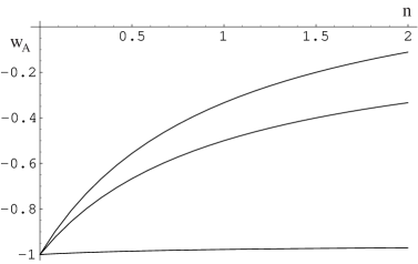
Figure 1: A plot of $w_{A}$, equation (19), for (from top to bottom) $\beta=1/2$ (radiation domination), $\beta=2/3$ (dust domination) and $\beta=15$ (nearly de Sitter inflation).

For later purposes, let me also discuss an approximate solution of the system (14). Suppose that $B\ll HA$ and $dV/dA\ll HB$. Loosely speaking, these inequalities are attained in the limits of large $A$ or large $H$. Then, equations (14) have the approximate solution

$$A=A_{(0)}\exp[-(N-N_{0})],\quad B=B_{(0)}\exp[-2(N-N_{0})]$$ (20)

Along this solution the kinetic energy of the field $B^{2}\propto e^{-4N}$ decreases, whereas the potential energy $V\propto e^{2nN}$ increases. Hence, soon the potential energy dominates the kinetic one, $B^{2}\ll V$, so that along this approximate solution the equation of state is

$$w_{A}\approx-1-\frac{2}{3}n,$$ (21)

which is less than $-1$. However, this approximate solution only holds temporarily, as the assumptions we have made finally become violated. Later on I will discuss an example where initial conditions place the triad on the approximate solution (20) for a significant period of time. Note that in the opposite limit, the limit where the kinetic energy dominates the potential one, $B^{2}\gg V$, the triad equation of state is radiation-like, $w_{A}\approx 1/3$. In both limits, the triad is quite different from a (canonical) scalar field (with positive potential), for which $-1\leq w\leq 1$.

III.2 Triad domination

Along the attractor (17), the energy density of the triad decays slower than the one of matter. Therefore, sooner or later the triad will come to dominate the universe. Consider thus the equation of motion (6) when the triad dominates the content of the universe. Using equations (7) and (9) the vector equation of motion (6) takes the form

$$\ddot{A}+3H\dot{A}+\frac{dW}{dA}=0,\quad\mathrm{where}\quad\frac{dW}{dA}\equiv\frac{4\pi G}{3}\left(12V-3\frac{dV}{dA}A\right)A+\frac{dV}{dA},$$ (22)

which is just like the equation of motion of a minimally coupled scalar with appropriate potential (we won’t need the explicit form of $W(A)$).

Solutions of equation (22) with constant $A=A_{*}$ can be easily identified by requiring $dW/dA$ to have a zero at $A_{*}$. This leads to the condition

$$\frac{d\log V}{d\log(4\pi GA^{2}-1)}\bigg{|}_{A_{*}}=2.$$ (23)

Those constant $A$ solutions are expected to be stable (attractors) if $d^{2}W/dA^{2}>0$, which implies

$$\frac{dV}{dA^{2}}+\frac{1}{4\pi G}\frac{d^{2}V}{d^{2}A^{2}}(1-4\pi GA^{2})\bigg{|}_{A_{*}}>0.$$ (24)

Along the attractor the energy density is, from equations (7a) and (9a),

$$\rho_{A}=\frac{3V(A_{*}^{2})}{1-4\pi G\,A_{*}^{2}},$$ (25)

i.e. a constant. Hence, these constant $A$ solutions are de Sitter attractors with ${w_{A}=-1}$; they are natural candidates to accommodate the present accelerated expansion of the universe. Figure 2 shows a phase diagram of the system (22) when the triad is the dominant component of the universe. Note that along the de Sitter attractor, the kinetic energy of the triad does not vanish.

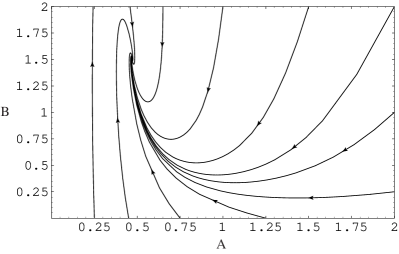
Figure 2: A phase diagram of the system (14) for $n=1/2$. The units are arbitrary. The diagram clearly shows that all phase trajectories converge to the single de Sitter attractor at constant $A$ and $H$.

Inserting the potentials (15) into equation (23) and verifying condition (24) I find that there is a single (stable) de Sitter attractor at

$$A_{*}^{2}=\frac{1}{4\pi G}\frac{n}{n+2}.$$ (26)

Substituting this value of $A_{*}$ into (25) and requiring it to be of the order of the present energy density, one can then estimate what is the required value of $M$ to fit the present stage of accelerated expansion,

$$M\sim 10^{-\frac{122}{4+2n}}G^{-1/2}.$$ (27)

Therefore, for $n\approx 0$ the required value leads to the “infamous” scale $M\sim 10^{-3}$ eV, whereas larger values of $n$ result into more reasonable energies. Note that we are fitting, rather that explaining, the time cosmic acceleration begins. As mentioned above, the exponent $n$ determines the value of the equation of state today. The close $n$ to $0$, the closer $w_{A}$ is to $-1$ today.

III.3 Two Examples

In this section I present two particular examples of possible realizations of vector dark energy. Current limits on the value of the equation of state of dark energy $w_{DE}$ and its derivative with respect to redshift $dw_{DE}/dz$ at $z=0$ are

$$w_{DE}\big{|}_{z=0}=-1.31\pm^{0.22}_{0.28}\quad\text{and}\quad\frac{dw_{DE}}{dz}\Big{|}_{z=0}=1.48\pm^{0.81}_{0.90},$$ (28)

where the prior on the density parameter of dust $\Omega_{M}=0.27\pm 0.04$ has been assumed Riess . Because the uncertainties are correlated, the reader is advised to look at the constraints on the $w_{DE}-dw_{DE}/dz$ plane in figure 10 of Riess . Note that the limits (28) are significantly weaker than the ones derived assuming that $w_{DE}$ is constant.

The first example has a potential

$$V(A^{2})=M^{4}\left(\frac{A^{2}}{M^{2}}\right)^{-1/4},\quad\textrm{where}\quad M^{9/2}=9\cdot 10^{-2}\left(\frac{3}{8\pi G}\right)^{5/4}H_{0}^{2}$$ (29)

and I am assuming that the Hubble constant today is $H_{0}=70$ km/s/Mpc. Note that in this model $V$ is not an analytic function of $A^{2}$. In particular, $A^{2}$ is constrained to be spacelike. Figure 3 shows the evolution of the energy density for different sets of initial conditions, and figure 4 shows the corresponding behavior of the triad equation of state. As clearly seen in the figures, the late time evolution of the cosmic triad is quite insensitive to initial conditions. For this particular model, $w_{A}\approx-0.87$, $dw_{A}/dz\approx 0.10$ and $\Omega_{A}\approx 0.72$ today. These values are consistent with the current limits on the properties of dark energy (28), see also figure 10 in Riess . Larger values of $n$ lead to violations of the limit on $w_{DE}$ today, whereas smaller values yield $w_{A}$’s closer to $-1$.

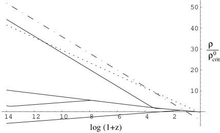
Figure 3: Triad energy density (in units of today’s critical energy density) versus $\log_{10}(1+z)$ for the interaction (29). Shown is the energy density of vector dark energy for four sets of initial conditions (continuous lines). For reference, the energy densities of radiation (dash-dotted) and dust (dotted) are also displayed. Note that despite the big difference in the initial value of the energy density (50 orders of magnitude), the present value of the dark energy density parameter still is $\Omega_{DE}\approx 0.72$.

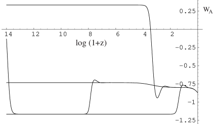
Figure 4: A plot of the triad equation of state for the same initial conditions and interaction as in figure 3. The attractors are easily identified by their constant value of $w_{A}$, which can be read off figure 1. For one set of initial conditions, the system reaches first the radiation attractor, then proceeds to the dust attractor and finally to the de Sitter attractor. For another, the system does not reach the radiation attractor, but does reach the dust one before continuing to the de Sitter solution. And lastly, for yet a different one the universe barely reaches the transition to the de Sitter attractor just in time. For all initial conditions, $w_{A}\approx-0.87$ today.

In the second example the interaction term is given by

$$V(A^{2})=M^{4}\left(\frac{A^{2}}{M^{2}}\right)^{-1/2},\quad\textrm{where}\quad M^{5}=\left(\frac{3}{8\pi G}\right)^{3/2}\,H_{0}^{2}.$$ (30)

This corresponds to $n=1/2$ in equation (15). In this case the triad evolution can be consistent with current observations if the initial value of $A$ is fine-tuned. The initial value of $B=(\dot{A}+HA)$ can be quite arbitrary though. Cosmic evolution for such a model and tuned initial conditions is shown in figures 5 and 6. The different lines correspond to different initial values of $B$. Note that all of them yield the same final result, and in particular all of them join the approximate solution (20). As seen in figure 6 the equation of state along that solution remains constant at $w_{A}=-4/3$ (equation (21)) all the way until today. By construction, in this particular example $w_{A}\approx-1.33$, $dw_{A}/dz\approx 0$ and $\Omega_{A}=0.72$ today. For integer values of $n$ and fine-tuned initial conditions it is also possible to obtain histories where the equation of state $w_{A}$ remains constant at a value significantly smaller than $-1$ for a long period of time, and just recently approaches $-1$. For these models $dw_{A}/dz$ tends to violate the limit in (28). Certain analyses of supernova data Starobinsky suggest that the equation of state has evolved from $w_{DE}\approx 0$ at $z\approx 1$ to $w_{DE}<-1$ today Starobinsky . Within the class of models (15) I have not been able to obtain such a behavior while keeping at the same time an early epoch of radiation domination.

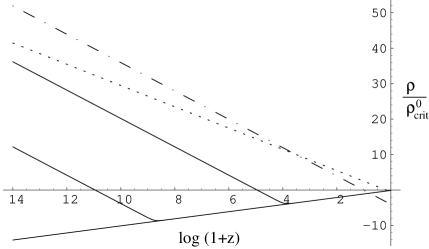
Figure 5: Triad energy density (in units of today’s critical energy density) versus $\log_{10}(1+z)$ for the second model (30). For reference, the energy densities of radiation (dash-dotted) and dust (dotted) are also displayed. The shown trajectories share the same initial value of $A$, though the initial values of $B$ are different. The present value of the dark energy density parameter is $\Omega_{DE}\approx 0.72$.

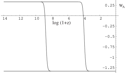
Figure 6: A plot of the triad equation of state of the dark triad for different initial conditions (same as in Figure 5). For all of them the triad reaches the equation of state $w_{A}=-4/3$, equation (21), and remains at that value till the present epoch.

IV Perturbations

The properties of any dark energy candidate not only comprise its equation of state, but also the way their perturbations (if any) behave Wayne . These perturbations are coupled through Einstein’s equations to metric perturbations, which in turn affect observables like CMB temperature anisotropies. The evolution of triad perturbations can also help to determine whether models with $w_{A}<-1$ suffer from serious instabilities and are hence unviable. Unfortunately, cosmological perturbation theory with a triad turns to be rather involved, as scalar, vector and tensor modes couple to each other. Therefore, in this section I only scratch the surface and mainly present qualitative features of the equations.

In scalar longitudinal gauge and vector gauge, the most general linearly perturbed spatially flat FRW metric is Bardeen ; KodamaSasaki ; MFB ; Wayne

$$ds^{2}=a^{2}(\eta)\left\{-(1+2\Phi)d\eta^{2}-2B_{i}\,d\eta dx^{i}+[(1-2\Psi)\,\delta_{ij}+2h_{ij}]dx^{i}dx^{j}\right\},$$ (31)

where $B^{i}$ is a transverse vector, $\partial_{i}B^{i}=0$, and $h_{ij}$ is a transverse and traceless tensor, $\partial_{i}h^{i}{}_{j}=h^{i}{}_{i}=0$. In a similar way, we can decompose the perturbations of the vector fields in the triad $\delta A^{a}_{\mu}$ into scalar and vector components,

$$\delta A^{a}_{\mu}=(\delta A^{a}_{0},\partial_{i}\chi^{a}+\delta A^{a}_{i}).$$ (32)

Here $\delta A^{a}_{0}$ and $\chi^{a}$ are scalars and $\delta A^{a}_{i}$ is a transverse vector, $\partial_{i}\delta A^{ai}=0$. Note that for convenience we are using conformal time. In the following, spatial indices are raised and lowered with the metric $\delta_{ij}$.

IV.1 Linearized triad equations

Because the vector fields in the triad do not couple to each other, we can study each of them at a time. Let me denote by $A^{a}_{i}$ the spatial components of one of the background triad vectors and let me drop in the following the index $a$. The $0$-component of the linearized equation of motion (3) in the spacetime (31) is

$$\left(\partial_{i}\partial^{i}-2a^{2}\frac{dV}{dA^{2}}\right)\delta A_{0}=-B_{i}A^{i}{}^{\prime\prime}-\partial_{i}(\Phi+\Psi)A^{i}{}^{\prime}+\partial_{i}\partial^{i}\chi^{\prime},$$ (33)

where a prime denotes a derivative with respect to conformal time. Remarkably, even though this is a scalar equation, it contains the vector perturbation $B^{i}$. In that respect, non-vanishing vector fields lead to violations of the decomposition theorem KodamaSasaki . In the absence of a background vector quantity, the only way to obtain a scalar linear in a vector $B^{i}$ is to compute its divergence $\partial_{i}B^{i}$, which vanishes for a transverse vector. However, if the spacetime contains a non-vanishing background vector $A_{i}$, it is possible to construct a scalar linear in a vector perturbation through the combination $A_{i}B^{i}$. The reason why the decomposition theorem is expected to hold in FRW universes is that in general they do not have any spatial direction singled out.

The $i$-components of the linearized equations have the form of the gradient of an equation that involves scalars plus an equation that involves transverse vector quantities. The scalar equation is

$$\chi^{\prime\prime}-\delta A_{0}^{\prime}-\delta=-2a^{2}\frac{dV}{dA^{2}}\chi,$$ (34)

where $\delta$ is implicitly defined by the decomposition

$$2\Phi A_{i}^{\prime\prime}+(\Phi+\Psi)^{\prime}A_{i}^{\prime}-2a^{2}\frac{d^{2}V}{d^{2}A^{2}}\delta(A^{2})A_{i}\equiv\partial_{i}\delta+\delta_{i},$$ (35)

into a scalar $\delta$ and a transverse vector $\delta_{i}$. The perturbation of $A^{2}$ is given by

$$\delta(A^{2})=2a^{-2}\left[A^{i}(\Psi\delta_{ij}-h_{ij})A^{j}+A^{i}(\partial_{i}\chi+\delta A_{i})\right],$$ (36)

and in particular, does not contain $\delta A_{0}$. The remaining vector equation takes the form

$$\delta A_{i}^{\prime\prime}-\partial_{j}\partial^{j}\delta A_{i}-(A^{j}{}^{\prime}\partial_{j})B_{i}-2h_{ij}^{\prime}A^{j}{}^{\prime}-\delta_{i}=-2a^{2}\frac{dV}{dA^{2}}\delta A_{i}.$$ (37)

Therefore, again, scalar, vector and tensor perturbations are not decoupled, since there exists a non-vanishing vector in the background.

Note that (33) is not a dynamical equation for $\delta A_{0}$, but a constraint. It seems that for tachyonic models, $dV/dA^{2}<0$, one cannot solve for $\delta A_{0}$, since in that case the operator $\partial_{i}\partial^{i}-2a^{2}dV/dA^{2}$ is not invertible. This would point out to a potential inconsistency of tachyonic models. However, as we shall see next, this difficulty is only apparent. Taking the Laplacian of equation (34) and using the time derivative of the constraint (33) to substitute the value of $\partial_{i}\partial^{i}\delta A_{0}^{\prime}$, one obtains a first order differential equation in time for $\delta A_{0}$ that does not contain its spatial derivatives,

$$\frac{dV}{dA^{2}}\delta{A_{0}}^{\prime}+\left[\left(\frac{dV}{dA^{2}}\right)^{\prime}+2\frac{a^{\prime}}{a}\frac{dV}{dA^{2}}\right]\delta A_{0}=f(\Phi,\Psi,\chi,a,\vec{A},\vec{B}).$$ (38)

Here, $f$ is a function of the specified variables and its derivatives we shall not be concerned with. What is important is that if a set of initial conditions satisfying the constraint (33) is specified, then, the solution of equations (38) and (34) is guaranteed to satisfy equation (33) at all times. Hence, it is in fact possible to solve for $\delta A_{0}$.

To conclude this part let us count how many “degrees of freedom” (per vector) the triad perturbations contain. We have seen that $\delta A_{0}$ is constrained, so it is not dynamical. Equation (34) contains the second time derivative of $\chi$ (1 dof) and equation (37) the second time derivative of the transverse vector $\delta\vec{A}$ (2 dof). Thus, there are $3$ degrees in freedom in total, as pertains to a massive vector.

IV.2 Perturbed Energy Momentum Tensor

The perturbations in the triad induce perturbations in its energy momentum tensor, which in turn are responsible for sourcing metric perturbations. In this subsection I shall deal with vector and tensor perturbations, which cannot be sourced in conventional cosmological models.

The perturbations in the energy-momentum tensor of the triad vectors $A^{a}_{\mu}$ can be decomposed into an isotropic pressure $\delta p_{A}$ and a traceless anisotropic stress $\Pi^{i}{}_{j}$ perturbation, $\delta T^{i}{}_{j}\equiv\delta p_{A}\delta^{i}{}_{j}+p_{A}\Pi^{i}{}_{j}$. The anisotropic stress itself can be decomposed into scalar, vector and tensor components, $\Pi^{i}{}_{j}\equiv{}^{(s)}\Pi^{i}{}_{j}+{}^{(v)}\Pi^{i}{}_{j}+{}^{(v)}\Pi_{j}{}^{i}+{}^{(t)}\Pi^{i}{}_{j}$, where ${}^{(s)}\Pi^{i}{}_{j}=(\partial^{i}\partial_{j}-\delta^{i}_{j}\partial^{k}\partial_{k}/3)\Pi$, ${}^{(v)}\Pi^{i}{}_{j}=\partial_{j}\Pi^{i}$ ($\Pi^{i}$ transverse), and ${}^{(t)}\Pi^{i}{}_{j}$ is transverse and traceless.

The equations of motion for vector (metric) perturbations are Wayne ; KodamaSasaki

$$\partial_{j}B^{i}{}^{\prime}+2\frac{a^{\prime}}{a}\partial_{j}B^{i}{}=8\pi Ga^{2}p_{A}{}^{(v)}\Pi^{i}{}_{j},$$ (39)

where ${}^{(v)}\Pi^{i}{}_{j}$ is the vector part of the triad anisotropic stress tensor. In the absence of anisotropic stress sources, equation (39) implies that vector perturbations decay away, $B^{i}\propto 1/a^{2}$. So even if they are generated in the early stages of the universe, they are not expected to be significant today. The transverse and traceless anisotropic stress sources tensor perturbations, i.e. gravitational waves,

$$h_{ij}{}^{\prime\prime}+2\frac{a^{\prime}}{a}h_{ij}{}^{\prime}-\partial^{k}\partial_{k}h_{ij}=8\pi Gp_{A}{}^{(t)}\Pi_{ij}.$$ (40)

As opposed to vector perturbations, in the absence of sources the amplitude of long-wavelength gravitational waves remains constant. Hence, if they are primordially produced, say during an inflationary stage, they could still have a sizable amplitude today.

I shall not write down all the terms that the perturbed spatial components of the energy momentum tensor of a single triad vector contains. They straightforwardly (but tediously) follow from the insertion of the perturbations (31) and (32) into equation (2). Instead, for the sake of illustration I shall consider only

$$\delta[{}^{a}T^{i}{}_{j}]=2a^{-2}\frac{dV}{dA^{2}}\left(A^{i}\delta A_{j}+\delta A^{i}A_{j}\right)+\cdots,$$ (41)

where the dots denote the multiple terms I am not explicitly writing down. In order to study the evolution of vector and tensor perturbations we have to compute the vector and tensor components of the previous expression. In Fourier space, these are given by KodamaSasaki

$$p_{A}{}^{(v)}\Pi^{i}=-\sum_{a}\frac{2ia^{-2}}{k^{2}}\frac{dV}{dA^{2}}(\vec{k}\cdot\vec{A}^{a})\,\delta A^{ai},$$ (42)

$$p_{A}{}^{(t)}\Pi^{i}{}_{j}=2a^{-2}\frac{dV}{dA^{2}}\sum_{a}\Bigg{[}A^{ai}\delta A^{a}_{j}+\delta A^{ai}A^{a}_{j} - \left(\frac{k^{i}}{k}\delta A^{a}_{j}+\delta A^{ai}\frac{k_{j}}{k}\right)\frac{\vec{k}\cdot\vec{A}^{a}}{k}-$$ (43)

$${}-\left(\delta^{i}_{j}-\frac{k^{i}k_{j}}{k^{2}}\right)\vec{A}^{a}\cdot\delta\vec{A}^{a}\Bigg{]},$$

which as required are transverse and traceless. Note that we sum over the three triad vectors to obtain the total energy momentum tensor perturbation. Because the triad perturbations $\delta{A}^{ai}$ are a priori totally independent from each other, the anisotropic stress ${}^{(t)}\Pi^{i}{}_{j}$ does not vanish in general. Thus, vector fields are not only expected to source vector perturbations, but also tensor perturbations. Again, the reason is that the decomposition theorem is violated. With the aid of the background vectors it is possible do construct traceless and transverse quantities linear in the perturbations.

If the perturbations have certain symmetries , ${}^{(t)}\Pi^{i}{}_{j}$ does indeed vanish (for the particular term in the energy momentum tensor we are considering). Because $A^{ai}$ and $k^{i}$ are the only vectors in the problem, the triad perturbation $\delta{A}^{ai}$ is expected to be a function of $A^{ai}$ and $k^{i}$. Since $\delta{A}^{a}$ is transverse, it has to be of the form

$$\delta{A}^{ai}=\alpha\cdot\left(\delta^{i}{}_{j}-\frac{k^{i}}{k}\frac{k_{j}}{k}\right)A^{aj}+\beta\cdot\varepsilon^{i}{}_{jk}A^{aj}k^{k},$$ (44)

where $\alpha$ and $\beta$ are two scalar functions and $\varepsilon_{ijk}$ is totally antisymmetric. Assume that $\alpha$ and $\beta$ do not depend on the index $a$ (that is, they do not depend on $k_{i}A^{ai}$.) Then, substituting equation (44) in (43) and using (5) one finds not only that ${}^{(t)}\Pi^{i}{}_{j}=0$, but also ${}^{(v)}\Pi^{i}=0$.

IV.3 Stability

The main worry one faces when dealing with tachyonic fields is their stability. In order to figure out to what extent the solutions we have found in Section III are stable, we should solve the system of cosmological perturbation equations just presented. Obviously, the coupling between scalar, vector and tensor perturbations makes this task quite formidable. In this section we dramatically simplify the equations by neglecting metric perturbations and concentrating on a particular set of vector modes. The hope is that this drastic simplification captures the qualitative features of the equations.

So let’s set $\Phi=\Psi=B^{i}=h_{ij}=0$ and consider the triad perturbation equations in Fourier space. From equation (35), for modes for which $\vec{k}\cdot\vec{A}=0$, it follows that $\delta=0$. Then, $\chi=\delta A_{0}=0$ is a solution of equations (33) and (34). Because $\delta_{i}\propto(A^{j}\delta A_{j})\,A_{i}$, if in addition we consider perturbations such that $\delta\vec{A}\cdot\vec{A}=0$, the remaining vector equation (37) reads

$$\delta\ddot{A}_{i}+H\delta\dot{A}_{i}+\frac{k^{2}}{a^{2}}\delta A_{i}+2\frac{dV}{dA^{2}}\delta A_{i}=0,$$ (45)

where for convenience I have gone back to cosmic time. Note how $2dV/dA^{2}$ plays the role of a mass term in the last equation. This is why I call interactions with $dV/dA^{2}<0$ “tachyonic”. Generically, if $dV/dA^{2}$ is negative, one expects growing modes, that is, instabilities.

In order to check the stability of the triad, it suffices to consider long-wavelength modes, $k=0$, in equation (45). For sufficiently high $k$, the gradient dominates the interaction and solutions are stable. Hence, any form of instability is an “infrared” effect, rather than an ultraviolet one. For a given expansion, equation (16), along the attractor (17), the long-wavelength solution of equation (45) is

$$\frac{\delta A_{i}}{a}=C_{+}\,t^{\gamma_{+}}+C_{-}\,t^{\gamma_{-}},\quad\text{where}\quad\gamma_{+}=\frac{1}{n+1}\quad\text{and}\quad\gamma_{-}=-3\beta+\frac{n}{n+1}.$$ (46)

Here, $C_{+}$ and $C_{-}$ are two integration constants and for convenience I have divided by the scale factor to obtain the length of the perturbation. We should compare these solutions with the behavior of the background, equation (17). Recall than $A$ is the common length of the background triad vectors. The $C_{+}$ mode in equation (46) grows as fast as $A$ and the $C_{-}$ mode grows less rapidly than $A$ if $n(1-3\beta)<1+3\beta$. Therefore, the $C_{-}$ mode decays relative to $A$ during inflation, radiation and dust domination. Hence, within the scope of our analysis, the system is not unstable throughout the period where the triad is subdominant. Note however that the triad would be unstable for certain values of $n$ if there had been a period of cosmic history during which $\beta<1/3$.

When the triad becomes dominant, the vector evolves towards the de Sitter attractor (26). The solution of equation (45) along the de Sitter attractor is

$$\frac{\delta A_{i}}{a}=C_{+}\exp(H_{*}t)+C_{-}\exp(-2H_{*}t),$$ (47)

where $H_{*}$ is the value of the Hubble constant along the de Sitter solution. Note that along the latter $A$ itself is constant. Thus, the de Sitter attractor is unstable, in the sense that $\delta A_{i}/a$ (the length of the vector perturbation) grows relative to $A$ (the length of the background vector). Because during the previous stages of cosmic history (when the triad was subdominant) the relative amplitude of the perturbations $\delta A/A$ has remained unaltered, the time perturbations become relevant will depend on early universe initial conditions. If the primordial vector amplitude agrees for instance with the (scalar) amplitude of density fluctuations, $\delta A/A\approx 10^{-5}$, $\delta A/A$ becomes of order one about $12$ $e$-folds after the onset of triad domination. By then the universe has presumably grown anisotropic, because there is no reason to expect that perturbations in the three different triad vectors are correlated. We’ll have to wait several billion years till that happens. At present the effect is still small, since the relative amplitude has increased at most by a factor of order one. In fact, it is tempting to speculate whether some of the anomalies observed in the CMB radiation quadrupole , specially in the quadrupole and octopole (see however low? ) and the related hints of statistical anisotropy non-isotropy , might be due to such an instability, which sets in once the universe starts to accelerate and mostly affects large scales.

V Summary and Conclusions

In this paper I have considered whether a vector field could be responsible for the current stage of cosmic accelerated expansion. The existence of a vector with non-vanishing spatial components turns to be compatible with the isotropy of a Friedmann-Robertson-Walker universe provided the vector is part of a “cosmic triad”, i.e. a set of three identical vector fields pointing in mutually orthogonal directions. A set of three identical self-interacting vectors naturally arises for instance in a gauge theory with $SU(2)$ or $SO(3)$ gauge group.

A distinctive property of a cosmic triad is that its equation of state of can become less than $-1$, even though its kinetic terms have the conventional form. The necessary condition is that the self-interaction is “tachyonic”, i.e. it naively gives rise to a negative squared vector mass. Although the simple analogy with scalar tachyons suggests that the study of tachyonic vectors is justified, there are also arguments that connect tachyonic vectors to phantom particles Dubovsky . In analogy to tracking quintessence models tracker , in this paper I have explored a particular class of tachyonic models, where the interaction is an inverse power-law. For appropriate initial conditions, there exist seemingly viable cosmologies where dark energy has an equation of state $w<-1$ throughout cosmic history, including today. In top of that, these models have attractors that render cosmic evolution quite insensitive to initial conditions and yield equations of state sufficiently close to $-1$ today. The experimental constraints on the value of the dark energy equation of state restrict the power of the vector self-interaction, while the time at which cosmic acceleration sets in determines its energy scale. Within the class of models I have considered, the current limits on the equation of state of dark energy require the vector self-interaction to be a non-analytic function of its squared length.

Finally, I have scratched the surface of cosmological perturbation theory in the presence of a cosmic triad. The most remarkable feature is the violation of the decomposition theorem. In the presence of a vector which has non-vanishing spatial components, scalar, vector and tensor perturbations do not decouple from each other. In particular, metric vector perturbations show up in scalar equations, and in the absence of particular symmetries in the perturbations vectors are able to source tensors. The (scalar) time components of the triad vectors are not dynamical, i.e. they are constrained. Despite an apparent difficulty, it is possible to solve the constraint also for tachyonic models. I have also considered solutions of the perturbation equations for a particular set of modes, under the assumption that metric perturbations are negligible. During inflation, radiation and dust domination the relative perturbations in the triad remain constant. However, there is a long wavelength instability during the late-time stage of de Sitter acceleration, where triad perturbations grow relative to the background. Hence, the time the universe becomes anisotropic depends on early universe initial conditions. For reasonable primordial perturbation amplitudes, the universe is expected to become anisotropic long time after the onset of cosmic acceleration. The instability of the triad during this epoch also suggests a possible relation between the large angle anomalies in the CMB sky and the onset of cosmic acceleration, but further work is needed to test this idea. A more careful investigation is also needed to establish whether tachyonic vectors are fully stable, and how the inclusion of metric perturbations affects the behavior of the triad perturbations (and vice versa).

To conclude, at the level of the present analysis it seems that vector fields could indeed be responsible for the present stage of late time cosmic acceleration, though it is yet unclear how quantum mechanics constrains the tachyonic models I have studied here.

*

Appendix A A Non-Abelian Triad Realization

In this appendix, I show that a cosmic triad can arise from a non-Abelian $SU(2)$ gauge theory. For that purpose, consider the gauge-invariant Yang-Mills Lagrangian

$$-\frac{1}{4}\int d^{4}x\sqrt{-g}\,F^{a}_{\mu\nu}F_{a}^{\mu\nu},$$ (48)

where $F^{a}_{\mu\nu}$ is the non-Abelian field-strength

$$F^{a}_{\mu\nu}=\partial_{\mu}A_{\nu}^{a}-\partial_{\nu}A^{a}_{\mu}+\varepsilon^{a}{}_{bc}A^{b}_{\mu}A^{c}_{\nu}.$$ (49)

The totally antisymmetric tensor $\varepsilon^{a}{}_{bc}$ encodes the structure constants of the $SU(2)$ Lie-algebra. The equations of motion of the fields in an arbitrary spacetime are

$$\frac{1}{\sqrt{-g}}\partial_{\mu}\left(\sqrt{-g}F^{a}{}^{\mu\nu}\right)+\varepsilon^{a}{}_{bc}A^{b}{}_{\mu}F^{c\mu\nu}=0.$$ (50)

The ansatz (5) satisfies these equations of motion in the FRW universe (4) if

$$\ddot{A}+3H\dot{A}+\left(H^{2}+\frac{\ddot{a}}{a}\right)A+\frac{dV}{dA}=0,$$ (51)

where

$$V=\frac{1}{2}\left(A_{\mu}A^{\mu}\right)^{2}.$$ (52)

Equation (51) agrees with the triad equation of motion (6). The energy momentum tensor of the gauge fields is

$$T_{\mu\nu}=F^{a}_{\mu\rho}F_{a}{}_{\nu}{}^{\rho}-\frac{1}{4}F^{a}_{\rho\sigma}F_{a}^{\rho\sigma}g_{\mu\nu}.$$ (53)

It can be verified that $T^{0}{}_{i}=0$, whereas

$$-T^{0}{}_{0}=\frac{3}{2}(\dot{A}+HA)^{2}+3V,\quad T^{i}{}_{j}=\left(\frac{1}{2}(\dot{A}+HA)^{2}-3V+2\frac{dV}{dA^{2}}A^{2}\right)\delta^{i}{}_{j}.$$ (54)

The self-interaction $V$ is again given by equation (52). Therefore, the energy density and pressure of the non-Abelian gauge fields agree with the ones of the triad, equations (9). This equivalence between the triad and the non-Abelian gauge fields in the symmetric case we are considering is confirmed by substituting the ansatz (5) into the actions (1) and (48). Note that for the triad vectors, as opposed to scalar fields or perfect fluids, the Lagrangian density is not the pressure nor the energy density. The existence and some properties of non-trivial solutions of general relativity coupled to an $SU(2)$ gauge field in a FRW universe have been considered in non-abelian .

References

- (1) A. G. Riess et al., “Type Ia Supernova Discoveries at From the Hubble Space Telescope: Evidence for Past Deceleration and Constraints on Dark Energy Evolution,” arXiv:astro-ph/0402512.
- (2) R. A. Knop et al., “New Constraints on , , and w from an Independent Set of Eleven High-Redshift Supernovae Observed with HST,” arXiv:astro-ph/0309368.
- (3) S. M. Carroll, “Why is the universe accelerating?,” arXiv:astro-ph/0310342.
- (4) G. R. Dvali, G. Gabadadze and M. Porrati, “4D gravity on a brane in 5D Minkowski space,” Phys. Lett. B 485, 208 (2000) [arXiv:hep-th/0005016].
- (5) S. M. Carroll, V. Duvvuri, M. Trodden and M. S. Turner, “Is cosmic speed-up due to new gravitational physics?,” arXiv:astro-ph/0306438.
- (6) M. S. Turner, “Dark matter and dark energy in the universe,” Phys. Scripta T85, 210 (2000) [arXiv:astro-ph/9901109].
- (7) C. Wetterich, “Cosmology And The Fate Of Dilatation Symmetry,” Nucl. Phys. B 302, 668 (1988). B. Ratra and P. J. E. Peebles, “Cosmological Consequences Of A Rolling Homogeneous Scalar Field,” Phys. Rev. D 37, 3406 (1988). R. R. Caldwell, R. Dave and P. J. Steinhardt, “Cosmological Imprint of an Energy Component with General Equation-of-State,” Phys. Rev. Lett. 80, 1582 (1998) [arXiv:astro-ph/9708069].
- (8) W. Hu and D. J. Eisenstein, “The Structure of structure formation theories,” Phys. Rev. D 59, 083509 (1999) [arXiv:astro-ph/9809368].
- (9) C. Armendariz-Picon, V. Mukhanov and P. J. Steinhardt, “A dynamical solution to the problem of a small cosmological constant and late-time cosmic acceleration,” Phys. Rev. Lett. 85, 4438 (2000) [arXiv:astro-ph/0004134].
- (10) T. Chiba, T. Okabe and M. Yamaguchi, “Kinetically driven quintessence,” Phys. Rev. D 62, 023511 (2000) [arXiv:astro-ph/9912463].
- (11) R. R. Caldwell, “A Phantom Menace?,” Phys. Lett. B 545, 23 (2002) [arXiv:astro-ph/9908168].
- (12) S. M. Carroll, M. Hoffman and M. Trodden, “Can the dark energy equation-of-state parameter w be less than -1?,” Phys. Rev. D 68, 023509 (2003) [arXiv:astro-ph/0301273].
- (13) J. M. Cline, S. y. Jeon and G. D. Moore, “The phantom menaced: Constraints on low-energy effective ghosts,” arXiv:hep-ph/0311312.
- (14) U. Alam, V. Sahni and A. A. Starobinsky, “The case for dynamical dark energy revisited,” arXiv:astro-ph/0403687. D. Huterer and A. Cooray, “Uncorrelated Estimates of Dark Energy Evolution,”arXiv:astro-ph/0404062.
- (15) L. Parker and A. Raval, “Non-perturbative effects of vacuum energy on the recent expansion of the universe,” Phys. Rev. D 60, 063512 (1999) [Erratum-ibid. D 67, 029901 (2003)] [arXiv:gr-qc/9905031].
- (16) A. Melchiorri, L. Mersini, C. J. Odman and M. Trodden, “The State of the Dark Energy Equation of State,” Phys. Rev. D 68, 043509 (2003) [arXiv:astro-ph/0211522].
- (17) H. Kodama and M. Sasaki, “Cosmological Perturbation Theory,” Prog. Theor. Phys. Suppl. 78, 1 (1984).
- (18) I. Zlatev, L. M. Wang and P. J. Steinhardt, “Quintessence, Cosmic Coincidence, and the Cosmological Constant,” Phys. Rev. Lett. 82, 896 (1999) [arXiv:astro-ph/9807002]. P. J. Steinhardt, L. M. Wang and I. Zlatev, “Cosmological Tracking Solutions,” Phys. Rev. D 59, 123504 (1999) [arXiv:astro-ph/9812313].
- (19) T. Kaluza, “On The Problem Of Unity In Physics,” Sitzungsber. Preuss. Akad. Wiss. Berlin (Math. Phys. ) 1921, 966 (1921). O. Klein, “Quantum Theory And Five-Dimensional Theory Of Relativity,” Z. Phys. 37, 895 (1926) [Surveys High Energ. Phys. 5, 241 (1986)]. Y. M. Cho and P. G. O. Freund, “Nonabelian Gauge Fields In Nambu-Goldstone Fields,” Phys. Rev. D 12, 1711 (1975).
- (20) J. D. Barrow, “Limits on cosmological magnetic fields and other anisotropic stresses,” arXiv:gr-qc/9712020.
- (21) F. Bunn, P. Ferreira and J. Silk, “How Anisotropic is our Universe?,” Phys. Rev. Lett. 77, 2883 (1996) [arXiv:astro-ph/9605123].
- (22) A. de Oliveira-Costa, M. Tegmark, M. Zaldarriaga and A. Hamilton, “The significance of the largest scale CMB fluctuations in WMAP,” Phys. Rev. D 69, 063516 (2004) [arXiv:astro-ph/0307282]. C. J. Copi, D. Huterer and G. D. Starkman, “Multipole Vectors–a new representation of the CMB sky and evidence for statistical anisotropy or non-Gaussianity at ,” arXiv:astro-ph/0310511. D. J. Schwarz, G. D. Starkman, D. Huterer and C. J. Copi, “Is the low-l microwave background cosmic?,” arXiv:astro-ph/0403353. D. L. Larson and B. D. Wandelt, “The Hot and Cold Spots in the WMAP Data are Not Hot and Cold Enough,” arXiv:astro-ph/0404037. P. Bielewicz, K. M. Gorski and A. J. Banday, “Low order multipole maps of CMB anisotropy derived from WMAP,” arXiv:astro-ph/0405007.
- (23) G. F. Smoot et al., “Structure in the COBE DMR first year maps,” Astrophys. J. 396, L1 (1992). N. Spergel et al., “First Year Wilkinson Microwave Anisotropy Probe (WMAP) Observations: Determination of Cosmological Parameters,” Astrophys. J. Suppl. 148, 175 (2003) [arXiv:astro-ph/0302209].
- (24) L. H. Ford, “Inflation Driven By A Vector Field,” Phys. Rev. D 40, 967 (1989).
- (25) T. Jacobson and D. Mattingly, “Gravity with a dynamical preferred frame,” Phys. Rev. D 64, 024028 (2001).
- (26) V. V. Kiselev, “Vector field as a quintessence partner,” arXiv:gr-qc/0402095.
- (27) W. Zimdahl, D. J. Schwarz, A. B. Balakin and D. Pavon, “Cosmic anti-friction and accelerated expansion,” Phys. Rev. D 64 (2001) 063501 [arXiv:astro-ph/0009353].
- (28) M. Novello, S. E. Perez Bergliaffa and J. Salim, “Non-linear electrodynamics and the acceleration of the universe,” arXiv:astro-ph/0312093.
- (29) D. Grasso and H. R. Rubinstein, “Magnetic fields in the early universe,” Phys. Rept. 348, 163 (2001) [arXiv:astro-ph/0009061].
- (30) C. M. Will, “Theory And Experiment In Gravitational Physics,” Cambridge University Press, UK (1981).
- (31) V. A. Kostelecky, R. Lehnert and M. J. Perry, “Spacetime-varying couplings and Lorentz violation,” Phys. Rev. D 68, 123511 (2003) [arXiv:astro-ph/0212003]. O. Bertolami, R. Lehnert, R. Potting and A. Ribeiro, “Cosmological acceleration, varying couplings, and Lorentz breaking,” Phys. Rev. D 69, 083513 (2004) [arXiv:astro-ph/0310344].
- (32) R. Lehnert, “Threshold analyses and Lorentz violation,” Phys. Rev. D 68, 085003 (2003) [arXiv:gr-qc/0304013].
- (33) S. M. Carroll, G. B. Field and R. Jackiw, “Limits On A Lorentz And Parity Violating Modification Of Electrodynamics,” Phys. Rev. D 41, 1231 (1990). D. Colladay and V. A. Kostelecky, “Lorentz-violating extension of the standard model,” Phys. Rev. D 58, 116002 (1998) [arXiv:hep-ph/9809521]. D. Bear, R. E. Stoner, R. L. Walsworth, V. A. Kostelecky and C. D. Lane, “Limit on Lorentz and CPT violation of the neutron using a two-species noble-gas maser,” Phys. Rev. Lett. 85, 5038 (2000) [Erratum-ibid. 89, 209902 (2002)] [arXiv:physics/0007049]. D. L. Anderson, M. Sher and I. Turan, “Lorentz and CPT violation in the Higgs sector,” arXiv:hep-ph/0403116.
- (34) S. M. Carroll, “Quintessence and the rest of the world,” Phys. Rev. Lett. 81, 3067 (1998) [arXiv:astro-ph/9806099].
- (35) C. Armendariz-Picon and V. Duvvuri, “Anisotropic inflation and the origin of four large dimensions,” Class. Quant. Grav. 21, 2011 (2004) [arXiv:hep-th/0305237].
- (36) V. F. Mukhanov, “Gravitational Instability Of The Universe Filled With A Scalar Field,” JETP Lett. 41, 493 (1985) [Pisma Zh. Eksp. Teor. Fiz. 41, 402 (1985)].
- (37) C. Armendariz-Picon, “Liberating the inflaton from primordial spectrum constraints,” JCAP 0403, 009 (2004) [arXiv:astro-ph/0310512].
- (38) S. L. Dubovsky, private communication.
- (39) E. C. G. Stueckelberg, “Die Wechselwirkung in der Eletrodynamik und in der Feldtheorie der Kernkräfte (Teil I),” Helv. Phys. Acta 11, 225 (1938). Id., “Die Wechselwirkung in der Eletrodynamik und in der Feldtheorie der Kernkräfte (Teil II und III),” Helv. Phys. Acta 11, 299 (1938).
- (40) H. Ruegg and M. Ruiz-Altaba, “The Stueckelberg field,” arXiv:hep-th/0304245.
- (41) S. Weinberg, “The Quantum Theory of Fields. Vol. 1,” Cambridge University Press (1995).
- (42) J. M. Bardeen, “Gauge Invariant Cosmological Perturbations,” Phys. Rev. D 22, 1882 (1980).
- (43) V. F. Mukhanov, H. A. Feldman and R. H. Brandenberger, “Theory Of Cosmological Perturbations. Part 1. Classical Perturbations. Part 2. Quantum Theory Of Perturbations. Part 3. Extensions,” Phys. Rept. 215, 203 (1992).
- (44) E. Gaztanaga, J. Wagg, T. Multamaki, A. Montana and D. H. Hughes, “2-point anisotropies in WMAP and the Cosmic Quadrupole,” Mon. Not. Roy. Astron. Soc. 346, 47 (2003) [arXiv:astro-ph/0304178]. G. Efstathiou, “A Maximum Likelihood Analysis of the Low CMB Multipoles from WMAP,” Mon. Not. Roy. Astron. Soc. 348, 885 (2004) [arXiv:astro-ph/0310207].
- (45) J. Cervero and L. Jacobs, “Classical Yang-Mills Fields In A Robertson-Walker Universe,” Phys. Lett. B 78, 427 (1978). M. Henneaux, “Remarks On Space-Time Symmetries And Nonabelian Gauge Fields,” J. Math. Phys. 23, 830 (1982). D. V. Galtsov and M. S. Volkov, “Yang-Mills Cosmology: Cold Matter For A Hot Universe,” Phys. Lett. B 256, 17 (1991).