Isothermal Shock Formation in Non-Equatorial Accretion Flows around Kerr Black Holes

Abstract

We explore isothermal shock formation in non-equatorial, adiabatic accretion flows onto a rotating black hole, with possible application to some active galactic nuclei (AGNs). The isothermal shock jump conditions as well as the regularity condition, previously developed for one-dimensional (1D) flows in the equatorial plane, are extended to two-dimensional (2D), non-equatorial flows, to explore possible geometrical effects. The basic hydrodynamic equations with these conditions are self-consistently solved in the context of general relativity to explore the formation of stable isothermal shocks. We find that strong shocks are formed in various locations above the equatorial plane, especially around a rapidly-rotating black hole with the prograde flows (rather than a Schwarzschild black hole). The retrograde flows are generally found to develop weaker shocks. The energy dissipation across the shock in the hot non-equatorial flows above the cooler accretion disk may offer an attractive illuminating source for the reprocessed features, such as the iron fluorescence lines, which are often observed in some AGNs.

1 Introduction

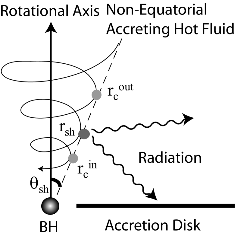
Figure 1: A side view of the schematic geometry in our model. A non-equatorial accreting fluid is conically accreting in the poloidal plane ($u^{\theta}=0$) onto the black hole, spiralling around the rotational axis $(u^{r}<0,u^{\phi}\neq 0)$ with a constant angle $\theta_{sh}$. It passes through the outer critical point $r^{out}_{c}$, gets shocked at $r_{sh}$ and passes through the inner critical point $r^{in}_{c}$ before reaching the horizon. The shock location $r_{sh}$ increases with increasing specific angular momentum of the fluid $\ell$. See the text for details.

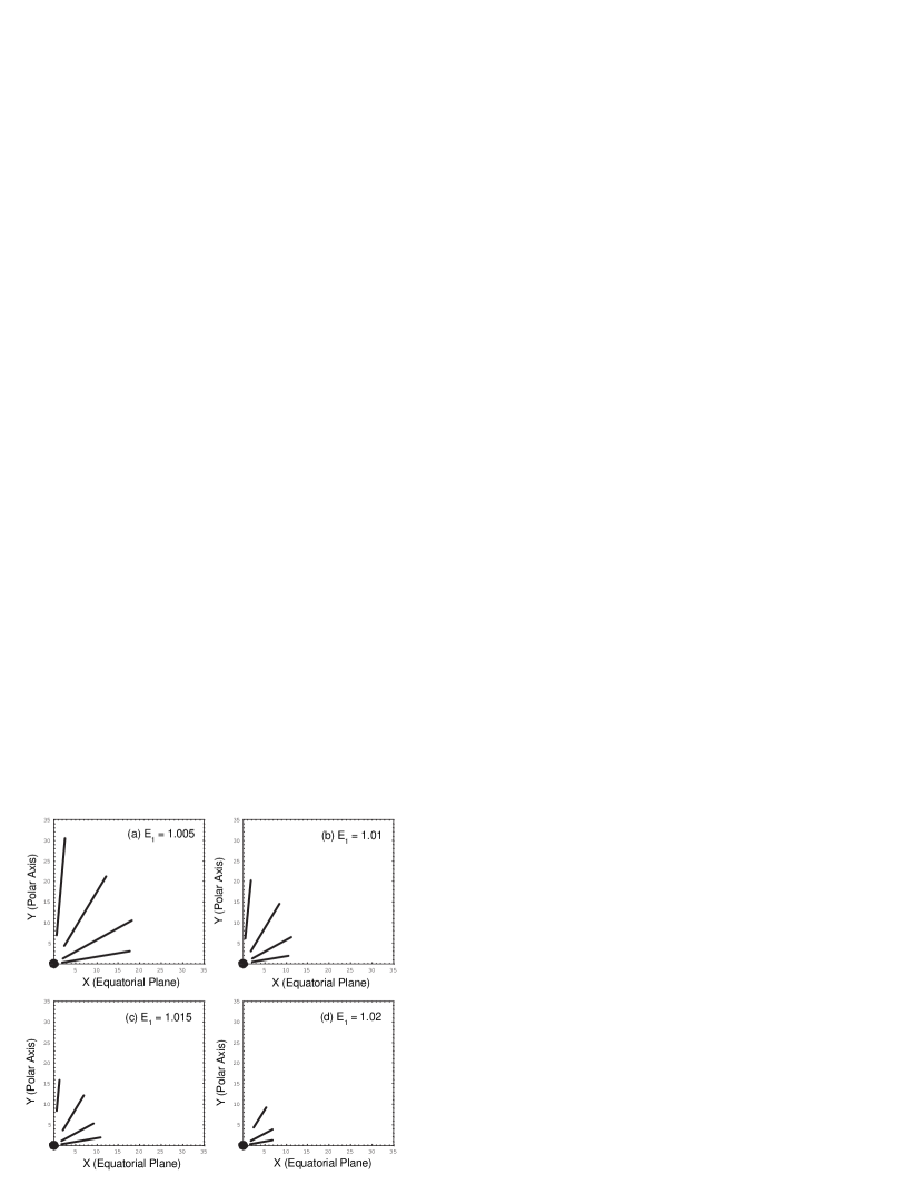
Figure 2: The range of isothermal, stable shock locations around a rapidly-rotating black hole ($a=0.99$ with prograde flows) for various angle $\theta_{sh}$ for fixed energy $E_{1}$. The black hole’s event horizon is $r_{h}=1.141r_{g}$ (central dot). No shock is found for $E_{1}=1.02$ with $\theta_{sh}=5\arcdeg$ in (d). Note that only the inner branch of shock locations are shown.

A realistic model of the AGN central engine may include the effects of the magnetic field. The black hole magnetosphere is studied first by Blandford & Znajek (1977) in the context of winds and jets from radio-loud AGNs. The work has been extended to magnetospheric physics of accreting AGNs by various authors (e.g., Phinney, 1983; Takahashi et al., 1990; Tomimatsu & Takahashi, 2001; Takahashi et al., 2002, hereafter TRFT02; Rilett et al.2004, in preparation). In this case, plasma particles should be frozen-in to the magnetic field lines, and hence the accreting fluid should fall onto the black hole from regions above the equatorial plane along the field lines(see, e.g., Figure 2 of TRFT02; Figure 1 of Tomimatsu & Takahashi, 2001). Then, magnetohydrodynamics (MHD) should become important to describe the motion of the particles associated with the background field. The resulting relativistic MHD shocks are explored by TRFT02 and Rilett et al. (2004, in preparation).

In general, the MHD shocks can be hydro-dominated or magneto-dominated (Takahashi, 2000, 2002, hereafter T02). Obviously the MHD case is, however, very complicated. Therefore, the main motivation of our current paper is, as a starting point, to investigate the hydrodynamic limit, which should be valid in the case of small magnetization. Here, we adopt a model which should apply to the hydro-dominated shocks where the magnetic field does not make a significant contribution to the properties of the shocks under a weak field limit, because in such a case hydrodynamics should primarily control the shock formation.

One-dimensional (1D), hot accretion flows around a black hole, generally treated as ideal hydrodynamical fluid, have been investigated by various authors (Sponholz & Molteni, 1994; Kato et al., 1996; Kato, Fukue, & Mineshige, 1998). It has been found that such accretion flows must be transonic, and will become supersonic before reaching the event horizon, while it is subsonic at infinity. Once such a fluid becomes supersonic, it is likely that a standing shock wave will develop when shock conditions are met. There are roughly three types of standing shocks: adiabatic (Rankine-Hugoniot) shocks, isothermal shocks, and isentropic compression waves (Abramowicz & Chakrabarti, 1990). The first attempt was made by Yang & Kafatos (1995) to self-consistently study the relativistic isothermal shock formation around black holes. In the case of isothermal shocks, the postshock fluid can lose substantial energy and entropy across the shock while the fluid temperature is continuous across the shock location (Lu & Yuan, 1997). Lu & Yuan (1998, hereafter LY98) examined the isothermal shock formation in one-dimensional (1D) adiabatic hot flows in the Kerr geometry, for various flow parameters including black hole rotation.

In our current paper, we extend the work by LY98 on isothermal shock formation in 1D adiabatic flows in the equatorial plane, to two-dimensional (2D) calculations for flows above the equatorial plane, to investigate geometrical effects. One of our major motivations is to explore the possibility that shocks produced in such flows act as a high energy radiation source for some reprocessed features, such as the iron fluorescent lines, which are observed from some AGNs. It is generally considered that a hot illuminating source above the cooler disk is required to produce such features (Fabian et al., 1989).

Section §2 introduces our basic equations and assumptions. The hydrodynamic fluid equations are solved in the context of general relativity. We discuss the isothermal shock conditions and the stability of shocks. The results are presented in Section §3 where we display shocks for various representative values of angular position, fluid energy, angular momentum, and black hole spin. Discussion and concluding remarks are given in the last section, §4.

2 Basic Equations & Assumptions

2.1 Background Kerr Geometry

The space-time is assumed to be stationary ($\partial/\partial t=0$) and axially-symmetric ($\partial/\partial\phi=0$) around a rotating black hole. The background Kerr metric is then expressed in the Boyer-Lindquist coordinates as

$$ds^{2} = -\left(1-\frac{2Mr}{\Sigma}\right)dt^{2}-\frac{4aMr\sin^{2}\theta}{\Sigma}\,dtd\phi$$ (1)

$$+\frac{A\,\sin^{2}\theta}{\Sigma}\,d\phi^{2}+\frac{\Sigma}{\Delta}\,dr^{2}+\Sigma\,d\theta^{2}\ ,$$

where $\Delta\equiv r^{2}-2Mr+a^{2}$, $\Sigma\equiv r^{2}+a^{2}\cos^{2}\theta$, $A\equiv(r^{2}+a^{2})^{2}-a^{2}\Delta\sin^{2}\theta$ with the metric signature being $(-,+,+,+)$. Throughout this paper, the distance is normalized by the gravitational radius $r_{g}\equiv GM/c^{2}$ where $c,G,M$ being the speed of light, gravitational constant, and the black hole mass, respectively. The hole’s event horizon is then $r_{h}\equiv(1+\sqrt{1-a^{2}})r_{g}$. Notice that $\theta=\theta_{sh}=\pi/2$ corresponds to the shocks in the equatorial plane while $\theta=\theta_{sh}\neq\pi/2$ denotes the non-equatorial shocks discussed here.

2.2 Hot, Adiabatic Fluid above the Equatorial Plane

Chakrabarti (1996a, b), Lu et al. (1997) and LY98 have studied general relativistic, equatorial flows in the Kerr geometry, whereas many of the previous works were based on the Pseudo-Newtonian potential (Paczynski & Wiita, 1980), which is not capable of reproducing the frame-dragging effect. To examine the two-dimensional (2D), relativistic hot accretion flow, here we assume an ideal, Boltzmann gas in a non-equatorial plane. Such an accreting fluid spirals around the symmetry axis due to angular momentum and accretes onto the black hole. The poloidal path of the fluid is assumed to be conical $(u^{\theta}=0)$ since the preshock fluid slowly starts falling from a distant location as a subsonic flow. That is, the fluid has only the radial velocity $(u^{r}<0)$ and the azimuthal velocity $(u^{\phi}\neq 0)$. Therefore, flow particles will spiral around the black hole rotation axis onto the hole. The schematic diagram of such an accreting fluid is displayed in Figure 1. The non-equatorial accreting fluid is conically falling onto the hole (i.e., $\theta$=constant and $u^{r}<0$ in the poloidal plane), spiralling around the symmetry axis in the azimuthal plane.

In this model perturbing forces to the fluid that might cause any acceleration in the $\theta$ direction is assumed to be negligible, keeping the flow at constant $\theta$ in a conical flow. This assumption is justified because we are exploring the weak field limit of MHD flows, which should apply to flows with small magnetization. As noted in Section §1 already, fluid particles in such flows should be frozen-in to the field lines and flow along the filed lines. Therefore, the flow geometry in our case is governed by the magnetospheric structure, rather than by the hydrostatic equilibrium of non-magnetic fluid. In this sense it is not appropriate, in our case, to adopt the approach of conventional, non-magnetic 2D thick accretion disk (or torus) models. Especially, it may be emphasized that our version of the ‘conical model’ is quite different from the conical equilibrium flow often adopted in conventional non-magnetic thick disk models.

Solving the geometry of the magnetospheric structure in a realistic manner is an extremely difficult problem, and only a very simple approximate version has been carried out (see, e.g., Tomimatsu and Takahashi 2001). Therefore, in our current paper which should apply to the weak field limit, we use, as our first approximation, the flow geometry we adopted already in our previous MHD accretions model where the infalling plasma is frozen-in to the radial field lines in a conical geometry, and hence the flows in different $\theta$ directions are decoupled from each other (see TRFT02, Rilett et al. 2004, in preparation).

Following the earlier works on relativistic accretion shocks, particularly LY98, we assume that a dynamical time-scale of the accretion process is much shorter than that for the energy (or thermal) dissipation during the fluid accretion. The fluid obeys the equation of state for an ideal gas

$$P={k_{B}\over\mu_{p}m_{p}}\rho T\ ,$$ (2)

where the primary thermodynamic property of the fluid is characterized by the locally measured temperature $T$ and the thermal pressure $P$. $\rho$, $\mu_{p}$ and $m_{p}$ are the rest-mass density of the fluid, the mean molecular weight of the composite particles and the mass of a particle, respectively. $k_{B}$ is the Boltzmann constant. The polytropic form is adopted as

$$P = K\rho^{\gamma}=K\rho^{1+1/n}\ ,$$ (3)

where the adiabatic index $\gamma$ is constant, and the polytropic index $n$ is correspondingly constant, too. We use $\gamma=4/3$ (or $n=3$) for our relativistic fluid. $K$ is a measurement of the entropy $S$ of the gas where $S\equiv c_{v}\log K$ ($c_{v}$ being a specific volume heat), expressed also via equations (2) and (3) as

$$K \equiv {k_{B}\over\mu_{p}m_{p}\rho^{\gamma-1}}T\ .$$ (4)

We consider the fluid to be stationary and axisymmetric. The fluid trajectory is conical in the poloidal plane and is spiralling around the polar axis onto the hole. Thus, $\theta$=constant or $u^{\theta}=0$, but $u^{r}<0$ and $u^{\phi}\neq 0$. Due to the space-time symmetry, specific total energy $E$ and axial angular momentum component $L$ of the fluid are conserved along the shock-free fluid’s path and are written as

$$E \equiv -\mu u_{t}\ ,$$ (5)

$$L \equiv \mu u_{\phi}\ ,$$ (6)

where $\mu=(P+\epsilon)/\rho$ is the relativistic enthalpy of the fluid, and $\epsilon=\rho+nP$ is the total energy-density including the internal energy term. With the use of the four-velocity normalization u $\cdot$ u $=-1$ where u = $(u^{t},u^{r},0,u^{\phi})$ is the four-velocity of the fluid, we find

$$1+u_{r}u^{r}+(u^{t})^{2}V_{eff}(r,\ell)=0\ ,$$ (7)

where $V_{eff}(r,\ell)\equiv g^{tt}-2\ell g^{t\phi}+\ell^{2}g^{\phi\phi}$ is called the effective potential (Lu, Yu, & Young, 1995) with $g^{\alpha\beta}$ being the Kerr metric tensor components. $\ell\equiv L/E=-u_{\phi}/u_{t}$ is the specific angular momentum of the fluid which is conserved along the whole flow if viscous dissipation is negligibly small (weak viscosity limit). Hence, we get $u_{t}$ in terms of $V_{eff}(r,\ell)$ as

$$u_{t}=\left(\frac{1+u_{r}u^{r}}{-V_{eff}}\right)^{1/2}\ .$$ (8)

On the other hand, the definition of the local sound speed is given by $c_{s}\equiv(dP/d\epsilon)^{1/2}$ following LY98, which is then rewritten as

$$c^{2}_{s}\equiv\frac{dP}{d\epsilon}=\left(1+\frac{1}{n}\right)K\rho^{1/n}\left(\frac{d\rho}{d\epsilon}\right)\ ,$$ (9)

and by definition of the enthalpy we also have

$$\mu=\frac{P+\epsilon}{\rho}=1+(1+n)K\rho^{1/n}\ .$$ (10)

Thus, combining equations (9) and (10), we find

$$1-nc^{2}_{s}=1-n\left(\frac{dP}{d\epsilon}\right)=\frac{1}{1+(1+n)K\rho^{1/n}}=\frac{1}{\mu}\ ,$$ (11)

where we now express the local sound speed in terms of the enthalpy (or vice versa). Accordingly, therefore, equation (5) can be rewritten as

$$E=\left({1+u^{r}u_{r}\over-V_{eff}}\right)^{1/2}/\left(1-nc^{2}_{s}\right)\ .$$ (12)

It is useful to notice here that both $E$ and $L$ will change across the shock location in the case of isothermal shock, but they change in such a way that the ratio $L/E$ (i.e., $\ell$) will stay unchanged (see a subsequent section). Notice that $K$ remains the same along the shock-free fluid due to the adiabatic assumption (no heat in/out), but does change across the shock. There is another constant along the fluid’s path called mass accretion rate $\dot{M}$. The spherical mass accretion rate is $4\pi r^{2}(-u^{r})\rho$ in the radial direction, and thus the mass accretion rate per unit spherical area by incoming fluid is given by

$$\dot{M}=r^{2}(-u^{r})\rho\ ,$$ (13)

which is constant along the whole flow. Since we are interested in shock formation where entropy is generated, let us follow LY98 and introduce another conserved quantity called the entropy accretion rate

$$\dot{\cal{M}}\equiv K^{n}\dot{M}=r^{2}\left[{c^{2}_{s}\over\gamma(1-nc^{2}_{s})}\right]^{n}(-u^{r})\ ,$$ (14)

where $\dot{\cal{M}}$ is conserved in a shock-free fluid, but changes in a shock-included fluid due to the entropy generation (i.e., $K$) at the shock location.

2.3 Regularity Conditions

It is known that any black hole accretion must be transonic (Chakrabarti, 1990a, 1996a), so it is important to locate the critical points (or sonic points to a particular observer) to make sure that the fluid is physically acceptable. Taking a derivative of equation (12) with respect to $r$, we obtain

$${du^{r}\over dr}={N\over D}\ ,$$ (15)

where

$$N \equiv {(u^{r})^{2}\over 2(1+u^{r}u_{r})}{dg_{rr}\over dr}-{2c^{2}_{s}\over r}-{1\over 2V_{eff}}{dV_{eff}\over dr}\ ,$$ (16)

$$D \equiv {c^{2}_{s}\over u^{r}}-{u_{r}\over 1+u^{r}u_{r}}\ .$$ (17)

In equation (15), $D(N=0)=0$ is required (regularity conditions) for $du^{r}/dr$ to be finite. Therefore, at critical points we get

$$c^{2}_{s}|_{c} = {u_{r}u^{r}\over 1+u_{r}u^{r}}|_{c}\ ,$$ (18)

$$c^{2}_{s}\left[{d(lng_{rr})\over dr}-4/r\right]|_{c} = {1\over V_{eff}}{dV_{eff}\over dr}|_{c}\ ,$$ (19)

where the subscript “c” denotes the critical points. Notice that the right-hand-side of equation (18) is the radial three-velocity component of the fluid measured by a corotating observer (this will be explained later). In other words, the critical points are equivalent to the sonic points only for such an observer. Multiple critical points (i.e., an inner point $r^{in}_{c}$, an intermediate point $r^{mid}_{c}$ and an outer point $r^{out}_{c}$) are known to exist in general for a set of $(E,\ell)$ (e.g., Chakrabarti, 1990b). This means that the location of the critical points will be different before and after the shock in a shock-included fluid since $E$ changes across the shock. The fluid must pass through a critical point on both sides of the shock. It is worth while to note that in isothermal shocks the postshock fluid cannot pass through the same critical points for the preshock fluid due to the energy dissipation at the shock location. This will be addressed more in a later section. Depending on the critical point that the fluid goes through, kinematic and thermodynamic profiles of the fluid will be different. In the framework of our model, however, it is not terribly important through which critical point the accreting fluid will pass as far as it produces a dissipative shock near the black hole. Therefore, we will only investigate the preshock fluid that passes through the outer critical point $r^{out}_{c}$ and the postshock fluid that passes through the inner critical point $r^{in}_{c}$.

2.4 Isothermal Shock Conditions

In our scenario the adiabatic fluid forms a standing shock (i.e., stationary shock location) somewhere between the preshock outer critical point $r^{out}_{c}$ and the postshock inner critical point $r^{in}_{c}$ on its way to the horizon. According to Abramowicz & Chakrabarti (1990), standing shocks in general can be categorized into three types: (1)adiabatic shocks or Rankine-Hugoniot shocks, (2)isentropic compression waves and (3)isothermal shocks. In the case of (1), the fluid by definition does not release any energy across the shock, carrying the generated entropy and its thermal energy with it (Fukue, 1987; Chakrabarti, 1990b; Lu et al., 1997). Thus, radiative cooling mechanism is extremely inefficient with the thermal energy being advected. In type (2), the shock radiates an energy equivalent to the generated entropy at the shock such that the entropy remains unchanged at the shock (Chakrabarti, 1989). In the case of type (3), a fraction of the preshock fluid’s energy and the entropy generated are lost from the fluid’s surface at the shock location such that the temperature (therefore the sound speed) remains continuous across the shock (Lu & Yuan, 1997, LY98). In other words, the dissipative cooling processes are so efficient that the energy is not advected with the fluid. A realistic shock could be between these two extremes (adiabatic and isothermal). However, in this paper we investigate case (3), because it is very interesting in the sense that a large amount of energy releases can be expected in the vicinity of the central black hole, which may be related to the observed emission features in AGNs.

Since the fluid total energy decreases across the isothermal shock, we have

$$E_{1} = \left({1+u_{1}^{r}u_{r1}\over-V_{eff}}\right)^{1/2}/\left(1-nc^{2}_{sh}\right)\ ,$$ (20)

$$E_{2} = \left({1+u_{2}^{r}u_{r2}\over-V_{eff}}\right)^{1/2}/\left(1-nc^{2}_{sh}\right)\ ,$$ (21)

$$E_{sh} \equiv E_{1}-E_{2}\ ,$$ (22)

where the subscript “1” and “2” denote a preshock and postshock quantity at the shock location, respectively. $c_{sh}\equiv c_{s}(r_{sh})$ is the local sound speed at the shock location. From the entropy accretion rate, we have

$$\dot{\cal{M}}_{1}=r^{2}_{sh}\left[{c^{2}_{sh}\over\gamma(1-nc^{2}_{sh})}\right]^{n}(-u^{r}_{1})\ ,$$ (23)

$$\dot{\cal{M}}_{2}=r^{2}_{sh}\left[{c^{2}_{sh}\over\gamma(1-nc^{2}_{sh})}\right]^{n}(-u^{r}_{2})\ .$$ (24)

Due to the shock formation, the fluid becomes hotter and entropy is generated at the shock front (i.e., mathematical discontinuity with zero-thickness). Thus, $\dot{\cal{M}}$ increases instantaneously at the shock location. However, the radiative cooling process may be so efficient that a fraction of the total entropy may be lost as radiation from the fluid surface. Therefore, the postshock temperature remains continuous and the postshock entropy becomes smaller than that of the preshock. That is, $T_{1}=T_{2}$ but $\dot{\cal{M}}_{1}>\dot{\cal{M}}_{2}$ although $\dot{M_{1}}=\dot{M_{2}}$. The radial momentum flux density is given by

$$F\equiv{c^{2}_{s}\over\gamma u_{r}}+u^{r}.$$ (25)

From conservation of momentum flux density in the radial direction, it is found that

$${c^{2}_{sh}\over\gamma u_{r1}}+u^{r}_{1}={c^{2}_{sh}\over\gamma u_{r2}}+u^{r}_{2}\ .$$ (26)

Based on the above jump conditions in addition to the regularity conditions, there are 9 equations (12), (14), (18), (19),  (20), (21), (23), (24) and (26) for 9 unknowns $r^{in}_{c}$, $r^{out}_{c}$, $r_{sh}$, $E_{2}$, $\dot{\cal{M}}_{1}$, $\dot{\cal{M}}_{2}$, $c_{sh}$, $u^{r}_{1}$ and $u^{r}_{2}$. Once a set of ($a,\theta_{sh},E_{1},\ell$) is specified, then the corresponding shock location $r_{sh}$ and all the other unknown quantities are uniquely determined. For the sake of completeness, it should be noted that any physically acceptable shocks in a transonic accretion flow must satisfy the boundary conditions ($r^{in}_{c}<r_{sh}<r^{out}_{c}$).

From equations (20) and (21), we note that $E_{1}>E_{2}$ at the shock location $r_{sh}$ because $|u^{r}_{1}|>|u^{r}_{2}|$. That allows some energy dissipation $E_{sh}$. Equations (23) and (24) also imply that the entropy accretion rate should decrease across the shock for the same reason. Now, we may extract some interesting qualitative implications from these equations. For example, we note that more energy release $E_{sh}$ should naturally be expected from strong shocks because a relatively large jump in the radial velocity $u^{r}$ across such shocks is made possible. Secondly, we clearly see the general trend for the effect of the direction, $\theta_{sh}$, on specific angular momentum of the fluid, $\ell$. For instance, $\ell$ cannot be large near the polar region since the centrifugal barrier is correspondingly small compared with that near the equator. Then, the non-equatorial fluid will have smaller rotational velocity $u^{\phi}$. Consequently, the flow could gain its radial component $u^{r}$ more efficiently than its azimuthal component $u^{\phi}$, which allows the preshock flow to become supersonic more quickly (or sooner) in the radial direction. The resulting shock location, therefore, will be further from the black hole for small $\theta_{sh}$ as compared with the shocks near the equator (large $\theta_{sh}$). Furthermore, the energy dissipation $E_{sh}$ from such (more distant) shocks will be small, due to the fact that only a small amount of fluid’s gravitational potential energy can be released, as opposed to a large amount of energy conversion from the gravitational potential in regions close to the hole. We will come back to this issue in Section §3.

As mentioned in the earlier section, the critical points $r_{c}$ are determined by the fluid parameters $(E,\ell)$. In dissipative shock-included flows, the preshock fluid energy $E_{1}$ (and $\dot{\cal{M}}_{1}$) decreases across the shock, which will subsequently determine the postshock critical points corresponding to different $E$. In other words, the postshock fluid with $(E_{2},\dot{\cal{M}}_{2})$ cannot pass through the critical points already determined by the preshock flow with $(E_{1},\dot{\cal{M}}_{1})$. Instead, new critical points for the postshock flow will be determined by the postshock flow parameter $(E_{2},\dot{\cal{M}}_{2})$. Therefore, one must find these new critical points based on $(E_{2},\dot{\cal{M}}_{2})$ for the postshock flows to describe global shock-included transonic flows. Such a flow topology will be illustrated in §3.5.

2.5 Stability Analysis

Although possible shock locations are found from the jump conditions, they need to be stable against a small perturbation. Otherwise, the shock will disappear as a result of a small change in its location. To check the stability, we perturb the radial momentum flux density (equivalent to pressure) by a small change in the shock location $r_{sh}$, a method originally developed by Yang & Kafatos (1995). Thus, a small perturbation of the momentum flux density is

$$\delta F_{2}-\delta F_{1}=\left({dF_{2}\over dr}-{dF_{1}\over dr}\right)\delta r\equiv\Delta\delta r\ .$$ (27)

When the momentum flux density is not balanced on both sides of the shock, the shock is not stable. Suppose that a shock location is slightly perturbed by $\delta r$. If $\Delta>0$ when $\delta r>0$ (or $\delta r<0$), the postshock momentum flux density becomes larger (or smaller) for accretion. Consequently, the shock location will be further shifted towards increasing (or decreasing) r, and the fluid will never find a stable shock location. If $\Delta<0$, on the other hand, the shock will always go back to the original location satisfying momentum equilibrium regardless of the sign of $\delta r$. Therefore, $\Delta<0$ is required for stable shocks for accretion.

2.6 Characteristics of Global, Shock-Included Flows

It is interesting to see how flow quantities are changing as the accreting gas falls onto the black hole. Here, we will estimate some of the important flow quantities for global, shock-included, transonic fluids as a function of radial distance $r$. First, we explore the kinematics of the flows through the four-velocity components $u^{r},u^{\phi}$ and the angular velocity $\Omega\equiv u^{\phi}/u^{t}$ as well. The physical flow velocity can be described by the radial three-velocity $v^{r}\equiv[u_{r}u^{r}/(1+u_{r}u^{r})]^{1/2}$ in a corotating reference frame (CRF) which is a locally-flat space. $v^{r}$ is known to be equal to the speed of light at the horizon. The Mach number is defined in CRF by $M\equiv v^{r}/c_{s}$. The relativistic enthalpy of the flow can be written as $\mu\equiv 1/(1-nc^{2}_{s})$ in the unit of fluid rest-mass energy (see equation (11)). The thermal pressure $P$ can be derived from equation (3) as $P\propto\rho^{\gamma}$. Then, the local temperature of the flow goes as $T\propto P/\rho$ using equation (2). By the mass conservation law, we get the local density of the flow as $\rho\propto 1/(r^{2}|u^{r}|)$. Here, we define a normalized pressure $\hat{P}\equiv P/K=\rho^{\gamma}$, temperature $\hat{T}\equiv P/\rho=k_{B}T/(\mu_{p}m_{p})$ and the mass density $\hat{\rho}\equiv\rho/\dot{M}=1/(r^{2}|u^{r}|)$, respectively.

3 Results

In this section we present our results and consider their physical implications. The obtained isothermal shock solutions are displayed for various parameters. Based on previous AGN observations and theoretical speculations (e.g., Iwasawa et al., 1996a, b; Wilms et al., 2001), the mass of the central supermassive black hole is chosen to be $M=10^{7}M_{\sun}$, and the hole is in general rapidly-rotating (i.e., an extreme Kerr black hole). We choose $a=0.99$ in most cases. However, in Section §3.4 the black hole spin dependence is investigated by adopting various values of $a$. The accretion fluid is rotating with the Keplerian angular velocity of $\Omega_{k}=1/(a+r^{3/2})$. We consider both direct flows ($a\ell>0$) and retrograde flows ($a\ell<0$).

As seen by LY98, we find stable, multiple shock locations ($r^{in}_{sh},r^{out}_{sh}$ where $r^{in}_{sh}<r^{out}_{sh}$) for the same set of parameters $(a,\theta_{sh},E_{1},\ell)$ satisfying all the requirements (i.e., shock jump conditions, boundary conditions, and stability analysis). The preshock flow which does not reach the event horizon is often called $\alpha$-type flow. In order for $\alpha$-type preshock flows to become physically acceptable, there must exist a shock. However, it is still uncertain through which shock location, between $r^{in}_{sh}$ or $r^{out}_{sh}$, the preshock flow will “transit” to the postshock flow (i.e., degeneracy of shocks). There may be some other physical conditions (for instance, viscous dissipation or magnetic field) that uniquely determine which shock is actually realized, but this is beyond the scope of this paper. To avoid complexity caused by the degeneracy, we will include only the inner range of shock locations $r^{in}_{sh}$ (which is closer to the hole). Although we are aware of the existence of the “degeneracy”, throughout this paper the outer range of shock locations are not considered. The reason is that, as mentioned already, our work is originally motivated by the X-ray observations of the “reprocessed features” such as the iron lines from some AGNs. These lines are considered to come from a cool accretion disk illuminated by a hot high energy radiation source above the disk plane. The whole system should, however, be very close to the central black hole(Fabian et al., 1989), because these lines often exhibit broadened features with a large gravitational redshift(Nandra & Pounds, 1994). Therefore, we are primarily interested in the inner shock formation close to the hole.

3.1 Isothermal Shock Locations above the Equatorial Plane ($0\arcdeg<\theta_{sh}<90\arcdeg$)

Solving the basic equations (conservation laws + shock conditions) introduced earlier, we found various stable shock locations for different fluid parameters such as ($\theta_{sh},E_{1},\ell$). The following four angles $\theta_{sh}$ are considered: $5\arcdeg$(near-axis region), $30\arcdeg$(lower polar region), $60\arcdeg$(upper equatorial region) and $80\arcdeg$(near equatorial region). The energy-dependence of the shock locations for various $E_{1}$ is also examined in the following manner: $E_{1}=1.005,~{}1.01,~{}1.015$ and $1.02$ for comparison where $E_{1}$ is expressed in the unit of the particle’s rest-mass energy $m_{p}c^{2}$. To avoid complications, we fix the black hole spin at $a=0.99$ (with the prograde flows). First, the cross-sectional distribution in the (X,Y)-plane of the obtained shock locations is displayed in Figure 2 where $E_{1}$ is (a)1.005, (b)1.01, (c)1.015 and (d)1.02 for the four selected $\theta_{sh}$ : $5\arcdeg,~{}30\arcdeg,~{}60\arcdeg$ and $80\arcdeg$ from top to bottom except for (d). As explained earlier, the outer range of shock locations is not shown there. It should be reminded that a different shock location $r_{sh}$ is accompanied by a different angular momentum $\ell$ in this figure. We will discuss this later in §3.3.

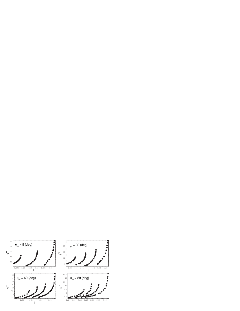
Figure 3: The shock location $r_{sh}$ versus angular momentum $\ell$ for various $E_{1}$ and $\theta_{sh}$ in the case of $a=0.99$ (with prograde flows). The dots represent the obtained shock locations. Each curve corresponds to the respective curves in Figure 2. From top to bottom, $E_{1}=1.005,~{}1.01,~{}1.015$ and $1.02$ except for $\theta_{sh}=5\arcdeg$ where no shock is found for $E_{1}=1.02$.

We find that the non-equatorial shock develops further away as $\ell$ increases for a fixed $E_{1}$ and $\theta_{sh}$, consistent with LY98 in the equatorial case. Both the inner critical point $r^{in}_{c}$ and the outer critical point $r^{out}_{c}$ will shift inward as $\ell$ increases for a fixed $E_{1}$ and $\theta_{sh}$. There exist a minimum $\ell$ ($\ell_{min}$) and a maximum $\ell$ ($\ell_{max}$) for each set of $(E_{1},\theta_{sh})$ for which the physically valid, stable shock formation is possible. In other words, the shock is unable to develop because of the violation of the boundary conditions and/or because of the instability under ceratin $\ell$ with $(E_{1},\theta_{sh})$. This is also commonly found in the equatorial shocks. The relation between the shock location $r_{sh}$ and the angular momentum $\ell$ for $a=0.99$ is seen in Figure 3 where $r_{sh}$ is plotted against $\ell$ for various angle $\theta_{sh}$. $E_{1}=1.005,~{}1.01,~{}1.015$ and $1.02$ from top to bottom except for $\theta_{sh}=5\arcdeg$ where $E_{1}=1.005,~{}1.01$ and $1.015$. Notice that infinitely many shocks do continuously exist between any two consecutive shocks plotted here although only representative shocks are shown (in dots) in this figure.

The range of the non-equatorial shock locations $\Delta r_{sh}$ in general tends to become narrower as $E_{1}$ increases for a fixed $\theta_{sh}$, where $\Delta r_{sh}\equiv r^{max}_{sh}-r^{min}_{sh}$. $r^{min}_{sh}$ and $r^{max}_{sh}$ are the innermost (smallest) shock location and the outermost (largest) shock location in the inner branch, respectively. From Figure 2, such a trend is obvious. For a fixed angle $\theta_{sh}$, the average location of the inner critical point $\bar{r}^{in}_{c}\equiv(r^{in}_{c,min}+r^{in}_{c,max})/2$ seems to be larger while the average location of the outer point $\bar{r}^{out}_{c}\equiv(r^{out}_{c,min}+r^{out}_{c,max})/2$ seems to be smaller as $E_{1}$ increases, where the additional subscript “min” and “max” denote the minimum value and the maximum value of the critical points for a fixed $E_{1}$ and $\theta_{sh}$, respectively. Another interesting feature with regard to the angular dependence is that $\Delta r_{sh}$ roughly becomes larger with decreasing $\theta_{sh}$ for a fixed $E_{1}$. That is, both the innermost shock location $r^{min}_{sh}$ and the outermost shock location $r^{max}_{sh}$ occur farther away from the hole when the accreting flow is nearer the polar region although $r^{max}_{sh}$ shifts outwards more than $r^{min}_{sh}$. This is because the average $r^{in}_{c}$ and the average $r^{out}_{c}$ both tend to become smaller with increasing $\theta_{sh}$. However, the degree of decrease in $r^{out}_{c}$ is much larger than that of $r^{in}_{c}$, which forces $\Delta_{sh}$ to be smaller with larger $\theta_{sh}$. Interestingly, no shocks can form when $E_{1}=1.02$ with $\theta_{sh}=5\arcdeg$ as seen in (d). This is due to the presence of the outer critical points very close to the black hole. With such a small $r^{out}_{c}$ (together with a certain value of $r^{in}_{c}$), there can be only a narrow (radial) region between $r^{in}_{c}$ and $r^{out}_{c}$. In the case of $5\arcdeg$ in (d), this region becomes so narrow that no jump conditions can be met within this range, resulting in no shock formations at all regardless of the angular momentum $\ell$.

As discussed in the earlier section §2.4, the average shock location seems to shift outwards with decreasing $\theta_{sh}$, which is qualitatively predicted as a result of a quick gain of the radial velocity due to smaller angular momentum $\ell$. In general, therefore, if the total preshock energy $E_{1}$ is relatively large when $\theta_{sh}$ is small, the formation of shocks may not necessarily be expected. In other words, the formation of shocks in a polar region may require less energetic hydrodynamic accretion fluid. The characteristic transition of these important locations are summarized in Table 1.

3.2 Properties of Dissipative Shocks

Figure 4 shows a three-dimensional plot where the shock location $r_{sh}$, the shocked fluid angle $\theta_{sh}$ and the shock strength $M_{1}/M_{2}$ are displayed for various $E_{1}$. We take $a=0.99$ (for the prograde flows) with $E_{1}=1.005,~{}1.01,~{}1.015$ and $1.02$ for (a), (b), (c) and (d), respectively. Here, $M_{1}/M_{2}$ is the fluid Mach number ratio just before the shock and just after the shock. For clarity purpose, the range of the plot varies from (a) to (d). Once again, no shock is found for $\theta_{sh}=5\arcdeg$ when $E_{1}=1.02$ (see panel (d)). For a global geometry of the whole shock location, refer to Figure 2.

One of the easily noticeable features in this figure is that $M_{1}/M_{2}$ increases with decreasing $r_{sh}$ down to a certain distance (peak radius $r_{p}$) and then turns to decrease inside $r_{p}$ for a fixed $E_{1}$. This is again the same pattern found in LY98 for $\theta$ = $90\arcdeg$ case. Such a trend can be seen more explicitly as $\theta_{sh}$ increases (compare $5\arcdeg$ and $80\arcdeg$, for instance). However, as $E_{1}$ increases, the rate at which $M_{1}/M_{2}$ increases outside $r_{p}$ seems to become smaller while the rate at which $M_{1}/M_{2}$ decreases inside $r_{p}$ appears to be larger for a fixed $\theta_{sh}$. That is, the slope of the $M_{1}/M_{2}-r_{sh}$ curve tends to become smaller with increasing $E_{1}$ (compare (a)1.005 and (d)1.02, for instance). Therefore, we can conclude that the preshock fluid with a small (large) $E_{1}$ and a large (small) $\theta_{sh}$ is more likely to produce a strong (weak) shock for a fixed shock location $r_{sh}$.

The energy dissipation $E_{sh}/E_{1}$ (or the ratio of the energy released to the preshock energy) from the preshock fluid is shown (in percent) as a function of $r_{sh}$ and $\theta_{sh}$ in Figures 5. The panels (a)-(d) correspond to the same energy $E_{1}$ as in Figure 4. This ratio basically follows the same pattern as the $M_{1}/M_{2}$ except for a specific detail. Since the $E_{sh}/E_{1}-r_{sh}$ curve qualitatively resembles the $M_{1}/M_{2}-r_{sh}$ curve, the energy dissipation $E_{sh}$ becomes larger as the shock occurs closer to the hole until the peak radius $r_{p}$ if it exists at all. The release of the energy from the hot flow tends to be more efficient when $\theta_{sh}$ is large for a fixed energy $E_{1}$, and the variation of $E_{sh}/E_{1}$ can be nearly an order of magnitude if the shock is developed near the disk plane (i.e., $\theta_{sh}\sim 90\arcdeg$) which can be seen in (a) and (b) in Figure 5. This can be qualitatively interpreted in terms of the energy conversion of the fluid, as we predicted in the section §2.4. The Shock developed further away can dissipate only a small gravitational potential energy whereas the shock close to the hole can convert more potential energy for dissipation. The maximum energy release can be as high as $\sim 18\%$ whereas the minimum energy release seems less than $1\%$ in the case of $a=0.99$ (with prograde flows). As another trend, more energy $E_{sh}$ tends to be released from a hot flow with a smaller $E_{1}$. Overall, it can be concluded that more energy release is expected from a low-latitude (i.e., large $\theta_{sh}$) hot flow with a small energy $E_{1}$.

3.3 Angular Dependence

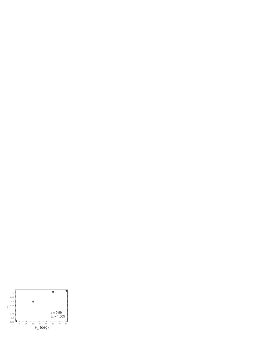
Figure 6: The specific angular momentum of the flow $\ell$ versus the angle $\theta_{sh}$. We take $\theta_{sh}=5\arcdeg,~{}30\arcdeg,~{}60\arcdeg$ and $80\arcdeg$. Each dot is a collection of many smaller dots that correspond to particular angular momentum at different radial shock locations $r_{sh}$. The other parameters are $a=0.99$ and $E_{1}=1.005$.

In order to see the angular dependence of the specific angular momentum of the shocked fluid, $\ell$, Figure 6 shows the $\ell$ versus $\theta_{sh}$ relation. We choose preshock fluid energy and black hole spin at fixed values, $E_{1}=1.005$ and $a=0.99$, respectively, in order to better understand the effects due to $\theta_{sh}$ alone. We find that at each $\theta_{sh}$, $\ell$ ranges from $\ell_{min}$ to $\ell_{max}$ for different radial shock location $r_{sh}$, (although it may be difficult to see this in the figure because $\ell_{mx}-\ell_{min}$ is much smaller than the variation of $\ell$ over $\theta_{sh}$). One can express the angular momentum as a function of $r-{sh}$, as $\ell=\ell(r_{sh})$. Note that LY98 also finds similar behavior (i.e., the $r_{sh}$ dependence of $\ell$). In fact, this is a general behavior found for any other shock-included global solutions. On the other hand, we note that for shock-free global accreting flows the $r$ dependence disappears, and hence a single value of $\ell$ should be determined by specifying $\theta$ alone.

We clearly see (in Figure 6) the general trend that the fluid angular momentum decreases with decreasing $\theta_{sh}$. That is physically consistent with the fact that the centrifugal force (due to the gravitational potential well) decreases towards the polar axis. Thus, the fluid must possess smaller angular momentum in the polar region (i.e., for small $\theta_{sh}$) for accretion to be realized. A similar trend has been found also in the work of the MHD shocks by TRFT02. It may be possible, in principle, to analytically show the dependence of the physically allowed angular momentum $\ell$ as a function of $\theta_{sh}$, for a given value of $r_{sh}$ (i.e., $\ell(r_{sh},\theta_{sh})$). However, that is beyond the scope of our present work. For our computation purposes these two variables ($\ell(r_{sh})$ and $\theta_{sh}$) are, to start with, treated as independent of each other. However, the valid solutions numerically found do indicate that $\ell$ is uniquely determined for a given set of the shock location ($r_{sh},\theta_{sh}$).

3.4 Black Hole Spin Dependance

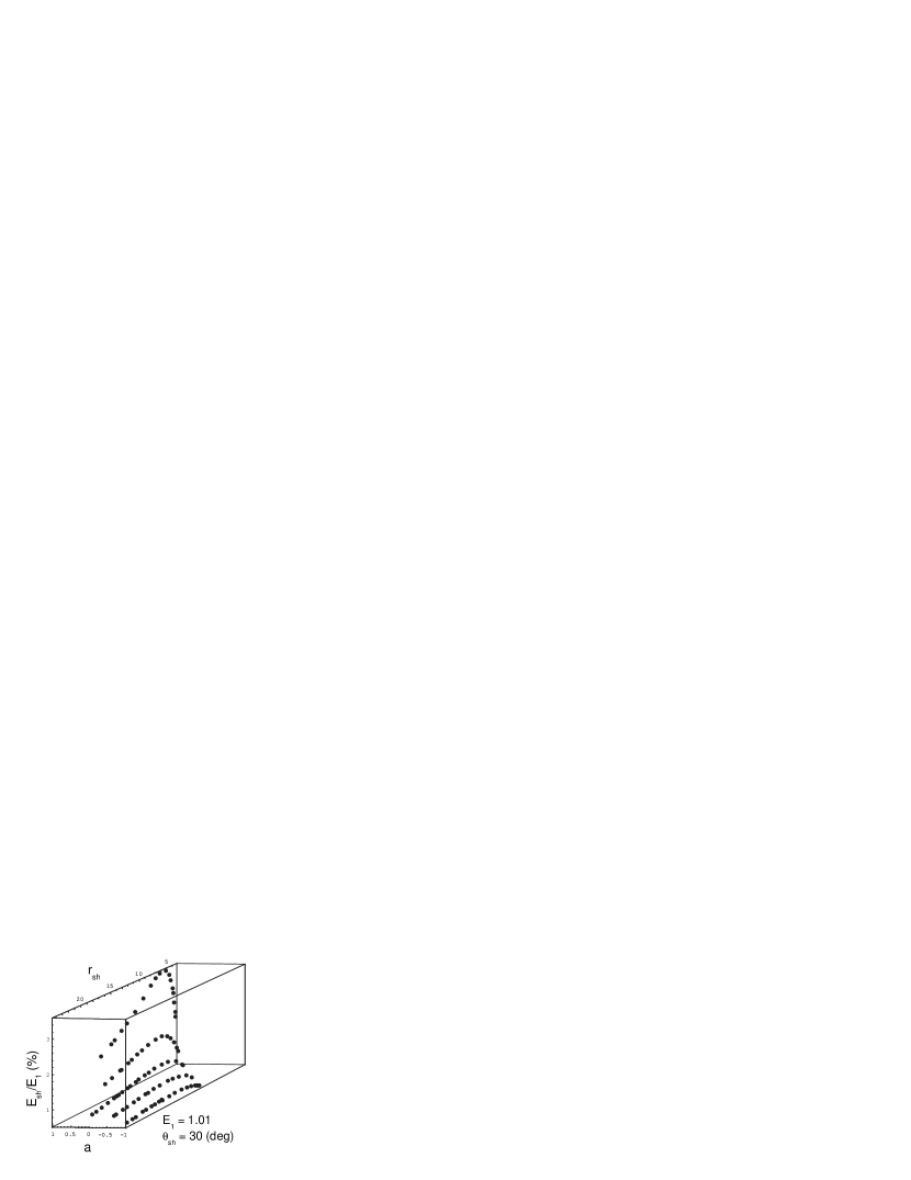
Figure 7: The energy dissipation ratio $E_{sh}/E_{1}$ (in %) as a function of the shock location $r_{sh}$ and the black hole spin $a$ for $E_{1}=1.01$ and $\theta_{sh}=30\arcdeg$. The dots represent the obtained shocks. We choose $a=-0.99,~{}-0.5,~{}0,~{}0.5$ and $0.99$. Negative black hole spin cases are considered to have retrograde flows (i.e., $a\ell<0$).

Here we explore the effect of black hole spin on shock properties. To decouple the effect of the hole spin from the other effects, we hold the fluid energy and the angle at fixed values of $E_{1}=1.01$ and $\theta_{sh}=30\arcdeg$, respectively. Figure 7 demonstrates the energy dissipation $E_{sh}/E_{1}$ (in %) as a function of the spin parameter $a$ and shock location $r_{sh}$. We take $a=-0.99,~{}-0.5,~{}0,~{}0.5$ and $0.99$. Since the fluid angular momentum $\ell$ is always taken to be positive here, the cases $a=-0.99$ and $-0.5$ refer to retrograde flows.

First we note that energy is most efficiently dissipated around a rapidly-rotating black hole in the presence of prograde flows. The retrograde flows with $a=-0.99$, on the other hand, appear to produce the least energy release, which corresponds to small Mach number ratio $M_{1}/M_{2}$. Due to the frame-dragging by the hole, the prograde flows can quickly acquire more velocity (especially the rotational component) in the course of its accretion, as opposed to the retrograde case where the fluid rotation appears even smaller (in the local inertial frame). Therefore, the prograde flows can afford more change in the kinetic motion at a shock location, and thus it may be “easier” for the prograde flows to dissipate more energy using the obtained kinetic motion. This viewpoint can be directly translated into the large Mach number ratio $M_{1}/M_{2}$ that we generally observe in the case of the prograde accretion. This may naturally explain large energy release $E_{sh}/E_{1}$ at shocks that we normally find. On the contrary, the retrograde flows generally cannot afford as much change as the prograde can in terms of the kinetic motion, and therefore only weak shocks can develop with small Mach number ratio (or small energy dissipation).

Keeping in mind that we are only interested in the inner range of the shocks here, the minimum shock location $r^{min}_{sh}$ tends to shift radially outwards with decreasing spin $a$. The maximum shock location $r^{max}_{sh}$ is the greatest when $a=0$. This suggests that in the retrograde flows no shock formations should be expected in a region very close to the hole, as opposed to the prograde case.

We can conclude from Figure 7 that very strong shocks (with more energy release) are expected in the inner region for the prograde flows.

3.5 Global Shock-Included Accreting Flow Solutions

As explained in Section §2.3, in the case of isothermal shocks, the global shock-included transonic solution must pass through the outer critical (sonic) point determined by the preshock parameters and simultaneously goes through the inner critical (sonic) point determined by the postshock parameters. Before looking into the detailed of particular flow dynamics, let us illustrate such a flow topology for a specific example. Figure 8 shows the Mach number $M$ of the transonic flow as a function of the radial distance $r$ (in logarithmic scale) for a shock-included transonic solution with $a=0.99,~{}\ell=1.463$ and $\theta_{sh}=30\arcdeg$. The preshock flow with $(E_{1},\dot{\cal{M}}_{1})=(1.01,5.27\times 10^{-5})$ goes through the outer critical point at $r^{out}_{c}=63.2r_{g}$, then makes the transition via the shock at $r_{sh}=11r_{g}$ into the postshock flow with $(E_{2},\dot{\cal{M}}_{2})=(0.98258,1.06\times 10^{-5})$ passing through the inner critical point at $r^{in}_{c}=2.58r_{g}$ before reaching the horizon. Notice that the preshock flow topology is completely independent of the postshock flow topology (both drawn in dark curves) in that they individually possess their own critical points (i.e., non-mutual points), and the flow transition from the former to the latter is allowed only through the shock (denoted in arrow). The other flows (shown in light gray curves) with different values of $\dot{\cal{M}}$ are unphysical solutions in terms of the fact that the jump conditions are not satisfied and that no critical points exist.

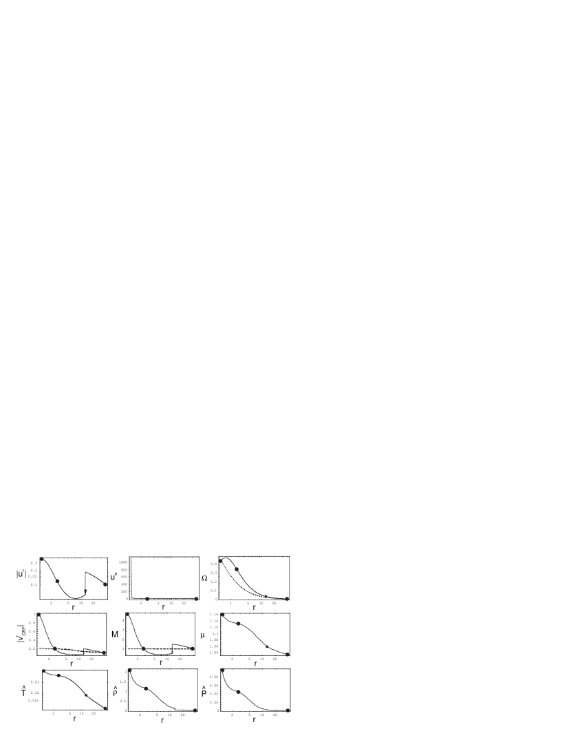
Figure 10: Global shock solutions for an adiabatic fluid (flow 2) with $E_{1}=1.015,\ell=1.4325,r_{sh}=12.75r_{g}$ for $\theta_{sh}=30\arcdeg$. The notations are the same as in Figure 9.

Here, we present three types of global, shock-included, transonic, accreting flow solutions in the case of $a=0.99$ (with prograde flows): Figure 9 for flow 1, Figure 10 for flow 2 and Figure 11 for flow 3. The flow parameters are tabulated in Table 2 for each flow. Each figure displays the radial component $|u^{r}|$ and the azimuthal component $u^{\phi}$ of the four velocity, the angular velocity $\Omega$ (solid curve) with the equatorial Keplerian velocity $\Omega_{kep}$ (dotted curve), the radial three-velocity in CRF $|v^{r}|$ (solid curve) with the local sound velocity $c_{s}$ (dotted curve), Mach number $M$, specific enthalpy $\mu$, flow temperature $\hat{T}$, local density $\hat{\rho}$ and thermal pressure $\hat{P}$ respectively. The enthalpy here is also normalized by the fluid rest-mass energy $m_{p}c^{2}$. The outer/inner critical (sonic) point is denoted by a large dot. The value at the event horizon is shown by another large dot. Either a vertical arrow or a small dot shows the transition from a preshock flow to a postshock flow through a stable isothermal shock. Note that $r_{hor}<r^{in}_{c}<r_{sh}<r^{out}_{c}$ for physically acceptable shocks. In Table 3, some representative fluid quantities for each flow is displayed in physical units. To make concrete calculations, we adopt the following relation between the (dimensionless) mass accretion rate for the non-equatorial hot gas ($\dot{m}_{hot}$) and the observed net accretion rate ($\dot{m}_{net}$) in the units of the Eddington mass accretion rate ($\sim 1.4\times 10^{25}$ g/s) for a $10^{7}M_{\sun}$ black hole mass. Here, we take $\dot{m}_{hot}\sim 0.01\dot{m}_{net}$ and $\dot{m}_{net}=0.1$ (relevant for radio-quiet AGNs) based on the assumption that the most of the accretion rate (99%) is contributed from the cool accreting gas in the accretion disk, whereas only a fraction of the net accretion rate ($\sim$ 1%) is due to the hot non-equatorial accreting fluid.

As seen in the earlier sections, flow 1 in Figure 9 goes through a relatively strong shock ($M_{1}/M_{2}\sim 5.4$) as a consequence of the dramatic increase in the density $\hat{\rho}$ and the pressure $\hat{P}$. The flow temperature $\hat{T}$ seems to be monotonically rising up to a peak point $r_{p}$ where the local sound speed is the maximum. In fact, all the thermodynamic quantities, such as $\mu$, $\hat{T}$ and $\hat{\rho}$, are all correlated to the sound speed. Notice that the local sound speed $c_{s}$ is continuous across the isothermal shocks because the flow temperature $\hat{T}$ is by definition continuous. Passing through $r_{p}$, the sound velocity starts decreasing which triggers a relatively large decrease in the thermodynamic properties such as $\mu$, $\hat{\rho}$, $\hat{P}$ and $\hat{T}$. The angular velocity $\Omega\equiv u^{\phi}/u^{t}$ roughly follows the Keplerian value (in the equator) almost all the way down to the horizon. The radial three-velocity $|v^{r}|$ appears to become maximum just before the shock and then transits through a strong shock, rising up again rapidly to become supersonic before entering the horizon. It is seen that, as expected, $|v^{r}|=1$ at the horizon.

Flow 2 in Figure 10 shows somewhat different behaviors compared to flow 1. First, the shock strength is weaker ($M_{1}/M_{2}\sim 3.0$). In terms of the kinematics, the angular velocity reaches a maximum value at some point and then slows down in the azimuthal direction from this point on. Notice that $\Omega(r)>\Omega_{k}$ for its entire trajectory. An interesting difference here is that the radial velocity is still decreasing after the shock for about $\sim 5r_{g}$ and then turns to pick up the (radial) speed. This is probably due to a relatively large shock location ($r_{sh}\sim 13r_{g}$). Thermodynamic quantities also behave in different ways here. After the shock, the flow temperature does not drop in this case. Instead, it continues to rise gradually just after the shock and the rate of the change becomes larger towards the horizon. This behavior is originating from the sound speed $c_{s}(r)$. The rest of the thermodynamic quantities ($\hat{\rho},~{}\mu$ and $\hat{P}$) also follow the same pattern.

The shock strength for flow 3 in Figure 11 is somewhere between flow 1 and flow 2 ($M_{1}/M_{2}\sim 4.8$). An outstanding feature in this case is a large deviation of $\Omega(r)$ from the Keplerian angular velocity in the equator. Since the shock location is relatively close to the hole, the postshock (radial) speed increases immediately after the shock. In both temperature and density profiles, a strange behavior can be seen after the shock. In temperature profile, the postshock fluid temperature appears almost constant producing a plateau-like pattern, whereas density profile $\hat{\rho}$ shows a step-like change in $\hat{\rho}$. Again, such a feature of these thermodynamic quantities can be explained by the sound speed $c_{s}(r)$.

It appears in general from the above three cases that the postshock fluid does not become supersonic right away if the shock is formed at a relatively distant location (say, $r_{sh}\gtrsim 10r_{g}$), in which case the radial velocity can be still slowing down. It turns out, however, that it is not easy to classify all the possible shock-included flows according to the angle $\theta_{sh}$ because the flow energy $E_{1}$ as well as the angular momentum $\ell$ are all certainly related to the flow dynamics, which allows a varieties of flow dynamics even for a fixed $\theta_{sh}$. For this reason, we will not try to simply attribute the above hydrodynamic/thermodynamic features in each flow to just one parameter out of ($E_{1},\ell,\theta_{sh}$).

4 Discussion & Concluding Remarks

Although our current work is partially motivated by the work of LY98, it also originates, in important ways, from our very recent work on black hole magnetospheres in accretion-powered AGNs - TRFT02 and Rilett et al. (2004, in preparation), where we explored adiabatic, relativistic MHD shocks produced in the black hole magnetosphere. We showed that strong shocks can indeed be formed in such flows for various relevant choices of flow parameters. In the current paper we extended these previous studies to explore the relativistic hydrodynamic flows which should apply to the case of weak magnetization. The reason is that the physics involved in the exact MHD case would be far more complicated, as noted already by TRFT02. Owing to these complexities, it was not straightforward for us to study the exact global shock-included MHD accretion flow solutions further in detail in a wider parameter/solution space.

As our next step, in the current paper we assumed a simple model of conical accretion flows, due to the fact that modelling more realistic flows (such as the ones in hydrostatic equilibrium) would be very complicated, especially in the framework of the relativistic non-equatorial accretions considered here. An appropriate force balance under the general relativistic geometry should be taken into account in more sophisticated models, but that is beyond the scope of our present work. We, however, would like to stress that our results still represents (at least qualitatively) important physical characteristics of shock formation in non-equatorial accretion flows. Also, in the presence of the magnetosphere, the fluid particles would be frozen-in to the field and hence flow along the field lines. For such a situation, application of conventional thick accretion disk (or torus) models is not appropriate.

We considered only the inner range of the shock formations in regions relatively close to the central engine, because of our interests in some X-ray observations of the reprocessed emission, such as the iron fluorescence lines, from some AGNs. Our results may offer the possibility of a high energy source in various broad regions ($0\arcdeg<\theta_{sh}<90\arcdeg$) above the disk plane. However, we find that the strongest shocks (high $M_{1}/M_{2}$ with large $E_{sh}$) should develop near the equator (large $\theta_{sh}$), although the quasi-polar shock (small $\theta_{sh}$) is also possible. We find no shocks in the polar region ($\theta_{sh}=5\arcdeg$) when the preshock fluid energy is relatively large although the shock-free accretion is physically allowed. The magnitude of the energy release from the shock roughly increases as the shock location gets closer towards the black hole, as already found by LY98 by their 1D studies. In addition, however, we further find, from our 2D calculations, that the shock-induced energy release $E_{sh}$ greatly depends, not only on the fluid energy $E_{1}$ and angular momentum $\ell$, but also on the angle of the shock location $\theta_{sh}$. The average shock strength (thus energy release) tends to be weaker towards the polar region.

Although TRFT02 considered adiabatic shocks and hence no energy dissipation, in the current paper we adopted the isothermal shocks because that ensures a substantial amount of energy release at the shock locations. Also, through the stability analysis our energy source (i.e., the shock) is found to be stable. Although we adopted adiabatic flows in our current work, it may be noted that Das, Pendharkar, & Mitra (2003) recently explored the isothermal shock formations in the isothermal flows, by adopting pseudo-Schwarzschild gravitational potentials and 1D equatorial flows. These authors concluded that their shocks also will release substantial amount of energy, which could be physically sufficient to become a radiation source for a strong X-ray flare.

In the present work, it is argued that a single isothermal shock formation between the two sets of accreting flows (preshock/postshock flows) is very likely with a substantial amount of energy dissipation. One may also ask whether it is possible to have a sequence of shock formations one after another in the course of the accretion. For example, a preshock flow with energy $E_{1}$ gets shocked at a shock location $r_{sh,1}$ becoming a subsonic postshock flow with energy $E_{2}$. The same flow with energy $E_{2}$ then becomes supersonic and develops another shock at $r_{sh,2}$ where $r_{sh,2}<r_{sh,1}$, making the transition to another subsonic postshock flow with energy $E_{3}$ where $E_{3}<E_{2}<E_{1}$. Such a sequential shock formation (namely “shock cascade” or “shock avalanche”) could be a very interesting phenomenon. Although discussion of such a possibility is beyond the scope of the present work, it is interesting, in a future work, to investigate such a possibility in relation to some observational applicability.

Before closing, we emphasize that a major justification for the choice of our version of a conical flow geometry follows from our recent work of TRFT02 on magnetospheric MHD accretion flows. However, here we adopted the hydrodynamic flows, as a limiting case of weak magnetization, in order to take advantage of the current fortunate situation that the relativistic hydrodynamic (equatorial) shocks in 1D accreting flows have already been extensively studied by many authors (e.g., Chakrabarti, 1989; Abramowicz & Chakrabarti, 1990; Lu et al., 1997; Lu & Yuan, 1997, and LY98). Our current investigation, however, is new and valuable in the sense that we have explored 2D non-equatorial shocks in a fully relativistic manner, with a possible application, for instance, to offer an attractive definite source for the energy dissipation in regions very close to the black hole.

Figure 4: Shock strength (Mach number ratio) $M_{1}/M_{2}$ as a function of the shock location $r_{sh}$ and the angle $\theta_{sh}$ for the same shocks as in Figure 2 ($r^{min}_{sh}\leq r_{sh}\leq r^{max}_{sh}$). The dots represent the obtained shocks. $E=1.005,~{}1.01,~{}1.015$ and $1.02$ for (a), (b), (c) and (d), respectively. We take $a=0.99$ with prograde flows.

Figure 5: The ratio of the energy dissipation to the preshock energy $E_{sh}/E_{1}$ (in %) for the same shocks as in Figure 2.

Figure 8: A flow topology of a global shock-included accreting flow with $E_{1}=1.01$ and $\theta_{sh}=30\arcdeg$ for $a=0.99$. A preshock transonic flow with $(E_{1},~{}\dot{\cal{M}}_{1})$ passing through an outer critical point $r^{out}_{c}$ develops an isothermal shock at $r_{sh}$ and becomes a subsonic postshock flow with $(E_{2},~{}\dot{\cal{M}}_{2})$. The flow then passes through an inner critical point $r^{in}_{c}$ becoming supersonic again before reaching the horizon. The physically valid preshock/postshock flows through the critical points are denoted by dark curves, while light grey curves refer to unphysical flows.

Figure 9: Global shock solutions for an adiabatic fluid (flow 1) with $E_{1}=1.02,\ell=2.104,r_{sh}=2.005r_{g}$ for $\theta_{sh}=80\arcdeg$. The horizon, inner and outer critical (sonic) points are respectively denoted by large dots from left to right in each figure. The shock is represented by either a small dot or a vertical arrow. From the upper-left panel to the upper-right panel, the radial component $|u^{r}|$ of the flow, the azimuthal component $u^{\phi}$ of the flow and the angular velocity $\Omega$ (solid curve) with the Keplerian value $\Omega_{kep}$ (dotted curve) are shown. From the middle-left panel to the middle-right panel, the radial three-velocity $|v^{r}|$ of the flow in the corotating reference frame (CRF) (solid curve) with the local sound velocity $c_{s}$ (dotted curve), the Mach number $M$ and the relativistic enthalpy $\mu$ are displayed. From the lower-left panel to the lower-right panel, the fluid local temperature $\hat{T}$, the density $\hat{\rho}$, and the thermal pressure of the flow $\hat{P}$ are plotted. For details, see Tables 2 and 3.

Figure 11: Global shock solutions for an adiabatic fluid (flow 3) with $E_{1}=1.005,\ell=0.2958,r_{sh}=6.95r_{g}$ for $\theta_{sh}=5\arcdeg$. The notations are the same as in Figure 9.

Table 1: Some Important Locations as a Function of $E_{1}$ and $\theta_{sh}$.

$E_{1}$	$\theta_{sh}$	$r^{min}_{sh}$	$r^{max}_{sh}$	$\Delta r_{sh}$	$\bar{r}^{in}_{c}$	$\bar{r}^{out}_{c}$
1.005	$5\arcdeg$	6.950	30.50	23.55	3.868	132.7
1.005	$60\arcdeg$	4.970	21.00	16.03	1.377	144.3
1.005	$80\arcdeg$	3.625	18.00	14.38	1.262	146.0
1.01	$5\arcdeg$	6.188	20.32	14.13	4.238	57.71
1.01	$60\arcdeg$	4.050	12.85	8.810	1.420	69.28
1.01	$80\arcdeg$	3.330	10.80	7.471	1.278	71.05
1.02	$30\arcdeg$	5.062	10.62	5.559	3.048	25.62
1.02	$60\arcdeg$	2.060	7.800	5.741	1.515	31.77
1.02	$80\arcdeg$	1.650	7.000	5.352	1.316	33.56

Note. — The length (or distance) is in the unit of $r_{g}$. See text for notations. $a=0.99$ for all cases.

Table 2: Global Shock-Included, Transonic, Non-Equatorial Accretions for Various Flow Parameters.

Flow	$E_{1}$	$\ell$	$\theta_{sh}$	$r_{sh}/r_{g}$	$r^{in}_{c}/r_{g}$	$r^{out}_{c}/r_{g}$	$M_{1}/M_{2}$	$\dot{\cal{M}}_{1}(10^{-5})$	$\dot{\cal{M}}_{2}(10^{-5})$	Figure
1	1.02	2.104	$80\arcdeg$	2.005	1.347	33.65	5.398	15.43	2.551	9
2	1.015	1.4325	$30\arcdeg$	12.75	2.697	37.85	2.987	9.265	3.046	10
3	1.005	0.2958	$5\arcdeg$	6.95	4.059	133.3	4.761	1.906	0.3896	11

Note. — $a=0.99$ for all cases. The black hole mass $M$ is $10^{7}M_{\sun}$.

Table 3: Thermodynamic Properties of Accreting Hot Flows at the Shock Location.

Flow	$E_{1}$	$\theta_{sh}$	$r_{sh}/r_{g}$	$c_{s}/c$	$n_{1}(10^{10}$)	$n_{2}(10^{10})$	$P_{1}(10^{5})$	$P_{2}(10^{5})$	Figure
1	1.02	$80\arcdeg$	2.005	0.2420	12.06	73.00	79.67	482.0	9
2	1.015	$30\arcdeg$	12.75	0.1351	0.4051	1.232	0.8335	2.535	10
3	1.005	$5\arcdeg$	6.95	0.1258	1.253	6.129	2.235	10.93	11

Note. — The subscripts “1” and “2” denote the preshock and postshock quantities, respectively. We adopt black hole mass $M=10^{7}M_{\sun}$, and $\dot{m}_{hot}=0.01\dot{m}_{net}=10^{-3}$. See the text for notations.

References

- Abramowicz & Chakrabarti (1990) Abramowicz, M. A., & Chakrabarti, S. K. 1990, ApJ, 350, 281
- Blandford & Znajek (1977) Blandford, R. D. & Znajek, R. L. 1977, MNRAS, 179, 433
- Chakrabarti (1989) Chakrabarti, S. K. 1989, PASJ, 41, 1145
- Chakrabarti (1990a) Chakrabarti, S. K. 1990a, Theory of Transonic Astrophysical Flows (World Scientific, Singapore)
- Chakrabarti (1990b) Chakrabarti, S. K. 1990b, ApJ, 350, 275
- Chakrabarti (1996a) Chakrabarti, S. K. 1996a, MNRAS, 283, 325
- Chakrabarti (1996b) Chakrabarti, S. K. 1996b, ApJ, 471, 237
- Das, Pendharkar, & Mitra (2003) Das, T. K., Pendharkar, J. K., & Mitra, S. 2003, ApJ, 592, 1078
- Fabian et al. (1989) Fabian, A. C., Rees, M., Stella, L., & White, N.E. 1989, MNRAS, 238, 729
- Fukue (1987) Fukue, J. 1987, PASJ, 39,309
- Iwasawa et al. (1996a) Iwasawa, K., Fabian, A. C., Mushotzky, R. F., Brandt, W. N., Awaki, H., & Kunieda, H. 1996a, MNRAS, 279, 837
- Iwasawa et al. (1996b) Iwasawa, K., Fabian, A. C., Reynolds, C. S., Nandra, K., Otani, C., Inoue, H., Hayashida, K., Brandt, W. N., Dotani, T., Kunieda, H., Matsuoka, M., & Tanaka, Y. 1996b, MNRAS, 282, 1038
- Kato et al. (1996) Kato, S., Inagaki, S., Mineshige, S., & Fukue, J. 1996, Physics of Accretion Disks (Gordon & Breach, New York)
- Kato, Fukue, & Mineshige (1998) Kato, S., Fukue, J., & Mineshige, S. 1998, Black-Hole Accretion Disks (Kyoto University Press)
- Lu, Yu, & Young (1995) Lu, J.-F., Yu, K. N., & Young, E. C. M. 1995, A&A, 304, 662
- Lu et al. (1997) Lu, J.-F., Yu, K. N., Yuan, F., & Young, E. C. M. 1997, A&A, 321, 665
- Lu & Yuan (1997) Lu, J.-F., & Yuan, F. 1997, PASJ, 49, 525
- Lu & Yuan (1998) Lu, J.-F., & Yuan, F. 1998, MNRAS, 295, 66 (LY98)
- Nandra & Pounds (1994) Nandra, K., & Pounds, K. A. 1994, MNRAS, 268, 405
- Paczynski & Wiita (1980) Paczynski, B. & Wiita, P. J. 1980, A&A, 88, 23
- Phinney (1983) Phinney, E. S. 1983, Ph.D.thesis, Univ. Cambridge
- Sponholz & Molteni (1994) Sponholz, H., & Molteni, D. 1994, MNRAS, 271, 233
- Takahashi et al. (1990) Takahashi, M., Nitta, S., Tatematsu, Y., & Tomimatsu, A. 1990, ApJ, 363, 206
- Takahashi (2000) Takahashi, M. 2000, in Proceedings of the 19th Texas Symposium on Relativistic Astrophysics and Cosmology, ed. E. Aubourg, T. Montmerle, L. Paul, & P. Peter (CD-ROM 01/27; Amsterdam:North-Holland)
- Takahashi (2002) Takahashi, M. 2002, ApJ, 570, 264
- Takahashi et al. (2002) Takahashi, M., Rilett, D., Fukumura, K., & Tsuruta, S. 2002, ApJ, 572, 950 (TRFT02)
- Tomimatsu & Takahashi (2001) Tomimatsu, A. & Takahashi, M. 2001, ApJ, 552, 710
- Wilms et al. (2001) Wilms, J., Reynolds, C. S., Begelman, M. C., Reeves, J., Molendi, S., Staubert, R., & Kendziorra, E. 2001, MNRAS, 328, L27
- Yang & Kafatos (1995) Yang, R., & Kafatos, M. 1995, A&A, 295, 238