Photoionization Modeling and the K Lines of Iron

Abstract

We calculate the efficiency of iron K line emission and iron K absorption in photoionized models using a new set of atomic data. These data are more comprehensive than those previously applied to the modeling of iron K lines from photoionized gases, and allow us to systematically examine the behavior of the properties of line emission and absorption as a function of the ionization parameter, density and column density of model constant density clouds. We show that, for example, the net fluorescence yield for the highly charged ions is sensitive to the level population distribution produced by photoionization, and these yields are generally smaller than those predicted assuming the population is according to statistical weight. We demonstrate that the effects of the many strongly damped resonances below the K ionization thresholds conspire to smear the edge, thereby potentially affecting the astrophysical interpretation of absorption features in the 7-9 keV energy band. We show that the centroid of the ensemble of K$\alpha$ lines, the K$\beta$ energy, and the ratio of the K$\alpha_{1}$ to K$\alpha_{2}$ components are all diagnostics of the ionization parameter of our model slabs.

1. Introduction

Iron K lines are of indisputable importance in astronomical X-ray spectra. They are unique among commonly observed X-ray lines in that they can be emitted efficiently by gas over a wide range of temperatures and ionization states. Their location in a relatively unconfused spectral region gives impetus to their use as plasma diagnostics. They were first reported in the rocket observations of the supernova remnant Cas A Serlemitsos et al. (1973), in X-ray binaries Sanford et al. (1975); Pravdo et al. (1977) and in clusters of galaxies Serlemitsos et al. (1977), the latter revealing the presence of extra galactic nuclear processed material. With the advent of orbiting X-ray detectors they were observed from almost all classes of astronomical sources detected in the 5-10 keV energy band. Further impetus for the study of these lines comes from observations of Seyfert galaxies and galactic black hole candidates, some of which show relativistically broadened and red-shifted lines attributed to formation within a few gravitational radii of a black hole Tanaka et al. (1995).

Recent improvements in the spectral capabilities and sensitivity of satellite-borne X-ray telescopes (Chandra, XMM–Newton) have promoted the role of Fe K lines as diagnostics, a trend that will continue with the launch of future instruments such as Astro-E2 and Constellation-X. Such plasma diagnostics ultimately rely on the knowledge of the micro physics of line formation and hence on the accuracy of the atomic data. In spite of the line identifications by Seely et al. (1986) in solar flare spectra and the laboratory measurements of Beiersdorfer et al. (1989, 1993), Decaux & Beiersdorfer (1993) and Decaux et al. (1995, 1997), the K-vacancy level structures of Fe ions remain incomplete as can be concluded from the critical compilation of Shirai et al. (2000). With regards to the radiative and Auger rates, the highly ionized members of the iso-nuclear sequence, namely Fe xviii–Fe xxv, have received much attention Jacobs et al. (1989), and the comparisons by Chen (1986) and Kato et al. (1997) have brought about some degree of data assurance. For Fe ions with electron occupancies greater than 9, Jacobs et al. (1980) and Jacobs & Rozsnyai (1986) have carried out central field calculations on the structure and widths of various inner shell transitions, but these have not been subject to independent checks and do not meet current requirements of level-to-level data and the needs for spectroscopic accuracy implied by recent and future astronomical instruments.

The spectral modeling of K lines also requires accurate knowledge of inner shell electron impact excitation rates and, in the case of photoionized plasmas, of partial photoionization cross sections leaving the ion in photoexcited K-vacancy states. In this respect, Palmeri et al. (2002) have shown that the K-threshold resonance behavior is dominated by radiative and Auger damping which induce a smeared edge. That is, photons at energies below the threshold for K shell ionization can excite from the ground state into np (3p, 4p, etc.) K-vacancy states. These then decay with a high probability by spectator Auger channels, in which the K vacancy is filled, and an ionization occurs, by electrons from the L shell. The excitation is a resonance with a width determined by the Auger and radiative lifetimes of the upper level, which can be quite short. This leads to multiple broad and overlapping resonances below the K edge, with combined strength which equals the K photoionization cross section. Spectator Auger decay has been omitted from many previous close-coupling calculations of high-energy continuum processes in Fe ions Berrington et al. (1997); Donnelly et al. (2000); Berrington & Ballance (2001); Ballance et al. (2001). An exception is the recent $R$-matrix computation of electron excitation rates of Li-like systems by Whiteford et al. (2002) where it is demonstrated that Auger damping is important for low-temperature effective collision strengths.

The present report is part of a project to systematically compute atomic data sets for the modeling of the Fe K spectra. The emphasis of this project is on both accuracy and completeness. For this purpose we make use of several state-of-the-art atomic physics codes, together with experimentally measured line wavelengths when available, to deliver for the K shell of the entire Fe isonuclear sequence: energy levels; wavelengths, radiative and Auger rates, electron impact excitation and photoabsorption cross sections. Most of this work has already been reported in a series of papers, organized loosely in order of descending ionization state: energy levels, transition probabilities and photoionization cross sections for Fe xxiv were reported by Bautista et al. (2003) (hereafter paper 1); energy levels and transition probabilities for the rest of the ’first row ions’ Fe xviii–Fe xxiii were reported by Palmeri et al. (2003a) (hereafter paper 2); energy levels and transition probabilities for the ’second row ions’ Fe x–Fe xvii were reported by Mendoza et al. (2004) (hereafter paper 3); properties of the photoionization cross sections and the role of damping by spectator Auger resonances were presented by Palmeri et al. (2002) (hereafter paper 4); energy levels and transition probabilities for the ’third row ions’ Fe ii–Fe ix were reported by Palmeri et al. (2003b) (hereafter paper 5); photoionization and electron impact cross sections were presented for the first row by Bautista et al. (2003) (hereafter paper 6); and photoionization cross sections for the second row by Bautista et al. (2004) (hereafter paper 7).

In the present paper we present a synthesis of all the data in the series and illustrate the application of these data to calculations of opacity and emission spectra of equilibrium photoionized plasmas. We explore the systematic behavior of the emission line profile shapes as a function of ionization parameter, the line emissivity as a function of gas density, column density and optical depth, and the absorption line and continuum properties as a function of ionization parameter. We show that the line profiles, although rich with detail, obey certain systematic behaviors. The K shell opacity also contains many features which depend on the ionization balance in the gas. Much of the data used for iron K shell which had been incorporated into previous models for the X-ray spectrum is shown to be overly simplified, and in some cases incomplete. All of the ingredients and results of the calculations published here are publicly available as part of the xstar photoionization code.

The models presented here are simple uniform slab models, but include an extensive suite of atomic data together with self-consistent ionization, excitation, and thermal balance. The resulting synthetic spectra are somewhat idealized, since they omit any density or pressure gradients and assume normal incidence for the illuminating radiation. They also use an approximate treatment of continuum Compton scattering, which is likely to be important at the large columns where iron K is emitted efficiently. Therefore they serve primarily as illustrations of the relative importance of various physical effects. These include the relative prominence of spectral features associated with damped lines, both in emission and absorption, and dependence of these quantities on ionization parameter and optical depth. More realistic synthetic spectra, involving accurate Comptonization in static atmospheres and winds, will be presented in a subsequent paper.

2. Model Ingredients

2.1. Atomic Data

The atomic data used in this are compiled from the data sets reported in the previous papers in the series, so we provide here only a brief summary of the assumptions and procedures used in the calculations. For the purposes of discussion, both here and elsewhere, the ions in the iron isonuclear sequence can be loosely classified according to the row in the periodic table associated with the various isoelectronic sequence. We emphasize, here and in what follows, that our goal is the treatment of the transitions and spectral features associated with the K shell of iron, so we have greatly simplified and omitted much of the physics associated with the outer shells in our calculations. We are confident that this does not significantly affect the accuracy of the results for the K shell, and we discuss reasons for this in what follows.

Computation of the atomic parameters for the iron ions requires taking into account the electron correlation and the relativistic corrections together. In our different studies detailed in papers 1–7, the approach we took is based on the use and comparison of results of several computational platforms, all of them publicly available, namely autostructure Badnell (1997)), hfr Cowan (1981), and the Breit–Pauli R-matrix package (bprm) based on the close-coupling approximation of Burke & Seaton (1971). While the latter was preferred for calculating the electron and photon scattering properties due to its accurate inclusion of the continuum channel coupling, the former two were chosen for their semi-empirical options which can utilize experimentally measured energy level spacings to improve the theoretical level separations for which the inter-system transition rates are sensitive. Although all these codes include relativistic effects and configuration interactions, autostructure has the most complete Breit Hamiltonian, i.e. the two-body part of the magnetic interactions. The Breit interaction plays a key role in the highly charged ions of the first row in particular for transitions with small rates and for those involving states subject to strong relativistic couplings. It was found that the energies and rates are also affected by core relaxation effects (CRE) and that these effects are more important than the higher order relativistic interactions for the spectator inner shell processes that dominate in the second and third row ions. Since, among the platforms used at the time this project was initiated, hfr handled CRE more efficiently in ab initio calculations (autostructure has since been updated to treat this process efficiently), it was used for data production in cases where no experimental level energies were available for the semi-empirical corrections, i.e. in the second and third row ions.

For the first row, a complete set of level energies, wavelengths, $A$-values, and total and partial Auger rates have been computed for the K-vacancy states within the $n=2$ complex. The experimental level energies listed in the compilation by Shirai et al. (2000) are used in semiempirical adjustment procedures. It has been found that these adjustments can lead to large differences in both radiative and Auger rates of strongly mixed levels. Several experimental level energies and wavelengths have been questioned as a result, and significant discrepancies are encountered with previous decay rates. These have been attributed to numerical problems in the older work. The statistical accuracy of the level energies and wavelengths is ranked at $\pm 3$ eV and $\pm 2$ mÅ, respectively, and that for $A$-values and partial Auger rates greater than $10^{13}$ s^-1 at better than 20%. Photoabsorption cross sections across the K edge and electron impact K-shell excitation effective collision strengths have also been calculated. The target models are represented with all the fine-structure levels within the $n=2$ complex, and the effects of radiation and spectator Auger dampings are taken into account by means of an optical potential Gorczyca & Badnell (2000). In photoabsorption, these effects cause the resonances converging to the K thresholds to display symmetric profiles of constant width that smear the edge with important implications in spectral analysis. In collisional excitation, they attenuate resonances making their contributions to the effective collision strength practically negligible.

Regarding the second-row ions, the K$\alpha$ and KLL Auger widths are found to be nearly independent of both outer electrons and electron occupancy keeping a constant ratio of $1.53\pm 0.06$. By comparing with previous theoretical and measured wavelengths, we estimate the accuracy of the reported wavelengths to be within 2 mÅ. Also, the good agreement found between the radiative and Auger data sets that are computed with different platforms allow us to propose with confidence an accuracy rating of 20% for the line fluorescence yields greater than 0.01. The predicted emission and absorption spectral features seem to be in good correlation with measurements in both laboratory and astrophysical plasmas. For computer tractability, photoionization cross sections across both the L and K edges have been computed in $LS$ coupling and later split among fine structure levels according to the formula of Rau (1976). Targets are modeled with all the singly excited terms within the $n=3$ complex. In similar fashion as for the first-row ions, the effects of radiative and Auger dampings are taken into account. Decaux et al. (1995) have published the only experimental study of the K-line spectrum of the Fe second row, and they found that the only ion for which the K lines are sufficiently unblended to derive accurate wavelengths is for Fe x. Their wavelengths for the doublet in the latter are approximately consistent with the ab-initio values computed by us and by Decaux et al. (1995).

There are no experimental data for Fe ions of the third row other than for Fe ii. For this ion, measurements have been made in the solid, and good agreement is found with our calculations. Level energies, wavelengths, $A$-values, Auger rates, and fluorescence yields have been obtained for the lowest fine-structure levels populated by photoionization of the ground state of the parent ion. Due to the complexity and size of level-to-level Auger calculations, we have employed a compact formula to compute Auger widths from hfr radial integrals Palmeri et al. (2001). An accuracy of $\sim$10% is estimated for the transition probabilities as a result of a comparison of K$\beta$/K$\alpha$ branching ratios taken from different theoretical and experimental data sets in the literature. Concerning the photoabsorption cross sections, a model similar to the one used in Paper 4 has been constructed whereby a single 1s $\rightarrow$ $n$p Rydberg series of Lorentzian resonances converging to each K threshold has been considered in each ionic species. The partial photoionization cross sections connecting the ground state of the parent ions to the different K-vacancy states have been calculated by autostructure in a single-configuration approximation.

In the present self-consistent photoionization model, we have incorporated all our published K-vacancy levels for the first-row ions and those populated by photoionization of the parent-ion ground state according to the selection rules of Rau (1976) in the case of species of the second and third rows. These are the levels whose populations are calculated explicitly and for which the transition rates given in our previous papers have been adopted. In addition superlevels are included that are associated with the photoabsorption features near the inner-shell edges using the bprm cross sections of Papers 6–7. The populations of these superlevels are also calculated, and their effects on the ionization and thermal balances are taken into account. Superlevel decays are treated as ‘fake’ transitions, i.e. lines with wavelengths much longer than any of interest to the model results. Such fake transitions are also used to treat the decays of other levels for which we do not explicitly treat the line wavelengths such as the decays of L-vacancy levels in the second and third row ions. Figure 1 shows two examples of energy-level diagrams: in Fe xviii, a typical case of a first row ion, and in Fe x which is representative of a second-row ion. In Fe xviii, the $[{\rm 1s}]{\rm 2p}^{6}\ {}^{2}{\rm S}_{1/2}$ K-vacancy state is populated by photoionization of the ${\rm 2p}^{6}\ {}^{1}{\rm S}_{0}$ ground state of Fe xvii. It then decays to or can be populated from the ground term ${\rm 2p}^{5}\ {}^{2}{\rm P}^{\rm o}$ through K$\alpha$ transitions. It can also decay via KLL Auger transitions or be populated by the inverse process, i.e. KLL dielectronic recombination from the ground configuration ${\rm 2p}^{4}$ of Fe xix. Photoabsorption near the K threshold is considered through a transition from the ground state to the [K] superlevel. That is, the full complexity of the energy dependent absorption cross section is calculated at all energies, but the portion below the K ionization threshold is used to calculate the photoexcitation rate into the [K] superlevel rather than as direct ionization. This $[K]$ superlevel can then decay to the ground or autoionize.

In the case of Fe x, the $[{\rm 1s}]{\rm 3p}^{6}\ {}^{2}{\rm S}_{1/2}$ K-vacancy state is populated by photoionization of the ${\rm 3p}^{6}\ {}^{1}{\rm S}_{0}$ ground state of Fe ix. It then decays either to the ${\rm 3p}^{5}\ {}^{2}{\rm P}^{\rm o}$ ground term through the K$\beta$ channel or to the $[{\rm 2p}]{\rm 3p}^{6}\ {}^{2}{\rm P}^{\rm o}_{1/2,3/2}$ L-vacancy states via the K$\alpha$ channel. It can also decay through Auger transitions, but here we neglect the dielectronic recombination channels from the ${\rm 3p}^{4}$ ground configuration of Fe xi because they involve only KMM autoionization rates which are orders of magnitude weaker than those of the main KLL Auger decay channels. We do not treat the cascade from L-vacancy states, and therefore the $[{\rm 2p}]{\rm 3p}^{6}\ {}^{2}{\rm P}^{\rm o}_{1/2,3/2}$ levels are connected to the ground levels with fake transitions. Photoabsorption near the K and L thresholds is considered via transitions that connect the [K] and [L] superlevels to the ground level. That is, we take the full absorption cross section including resonance structures from the $R$-matrix calculations, and attribute this part of it to photoexcitation into these superlevels. The photoionization transition to the [L] superlevel is associated with small contributions of L-shell channels to the cross section near the K edge. These contributions cascade through Auger decays to the ground level of the neighboring ion, here Fe xi. In the third row, the K-vacancy states decay to L-vacancy states (K$\alpha$ lines) and to 3p subshell vacancy states (K$\beta$ lines). The former are populated exclusively by photoionization from the ground level of the parent ion. We have applied the same treatment of the cascade as for the second-row ions. The L-vacancy and 3p-vacancy levels decay to the ground level through fake transitions. The photoabsorption near the K edge is described in terms of a single 1s $\rightarrow$ $n$p Rydberg series converging to the different K thresholds.

Figures 2–3 plot the energies of the lines and K edges in our data set as a function of ionization stage which can be compared with those presented by House (1969) and by Makishima (1986). For each ion the energies of all the components of a line or a K photoionization edge are plotted with equal weight and without accounting for broadening due to damping or blending into an unresolved transition array (UTA). So the dispersion in the line or photoionization threshold-energy for each ion represents the range in centroid energies of various lines or continua. This does not take into account the broadening due to damping or the relative strengths of the various components arising from the distribution of upper-level populations and transition probabilities. In Section 2.2 synthetic profiles are presented which take these factors into account. The distinction between the low and high ionization stages is apparent: for the third row the dispersion in line and K-threshold energies within a given ion can be comparable to the difference in these quantities between adjacent stages although the K$\beta$ line provides a sensitive diagnostic of the charge state. For example, the K$\alpha$ energies are in the range 6385–6403 eV in Fe ii–vii. For Fe viii–xi, the K$\alpha$ energy interval actually decreases slightly to 6381–6403 eV. This is somewhat counter-intuitive since generally binding energies increase with increasing ionization causing all line energies to increase. However, the K$\alpha$ lines are sensitive to both the 1s and 2p electron binding energies. The former does increase with increasing ion stage while the 2p energy decreases slightly due to the changing interaction with the 3d shell electrons. Further evidence for this comes from the fact that the K$\beta$ line energy increases between Fe i and Fe xi as the K$\alpha$ energy decreases. For Fe xii–xiii the line intervals increase to 6380–6415 eV, for Fe xiv–xv increasing by approximately 3 eV per ion from 6385–6422 eV to 6391–6428 eV. Fe xvi has a particularly simple structure owing to its Na-like configuration, with lines at 6414 eV and 6426 eV. For the first row, K$\beta$ is unimportant, and there is much greater separation between various ion stages. Each ion stage has line energies ranging over $\sim$200 eV. Note that some first-row ions can emit lines at energies below 6.4 keV; for example, transitions such as ${\rm 1s2s}^{2}{\rm 2p}^{4}-{\rm 1s}^{2}{\rm 2p}^{5}$ in Fe xix produce lines near 1.99 Å (6.23 keV). These transitions are strongly affected by configuration interaction with, for instance, ${\rm 1s}^{2}{\rm 2s}^{2}{\rm 2p}^{3}$ and have relatively small $A$-values ($\sim$10¹² s^-1).

Each bprm cross section in Papers 6–7 (first and second row ions) is tabulated on an energy grid containing several thousand points. In order to include these data into the xstar database, compression is invoked using the resonance-average photoionization (RAP) method and the numerical representation of RAP cross sections proposed by Bautista et al. (1998). The choice of the accuracy parameter ($\Delta\equiv\delta E/E$) is guided by the instrumental resolution of the XRS on board ASTRO-E2 at the energies of the iron K lines, i.e. $\Delta=0.0001$ (10 times the XRS resolving power at 6.4 keV). Figure 4 plots the photoabsorption cross sections for the various ions, and in Table 2 we give the strongest near K-edge absorption features that can be resolved by the XRS (resolving power of 1000). Each feature can be due to a superposition of several resonances; the feature parameters, namely wavelength, oscillator strength, and full width at half maximum, are fitted values extracted from Gaussian profiles using RAP cross sections with $\Delta=0.001$.

Examination of Figure 4 shows a variety of different cross-section behaviors, depending crudely on ionization stage (i.e. first, second, or third row) and on the fine structure of both the valence- and inner-shell electron configurations. In the third row, resonance features are close to the threshold often overlapping and K$\alpha$ and K$\beta$ do not appear. The second row shows more complex behavior, and K$\beta$ also appears in absorption. In the first row both K$\alpha$ and K$\beta$ appear in absorption, along with a very rich and distinct resonance spectrum below threshold. More details of the resonance features and a description of the level scheme adopted for each ion are given in the Appendix.

2.2. xstar

Results in the following section were calculated by incorporating the K vacancy energy levels, and the transitions connecting them to other states of the ions of iron, into the xstar modeling code (Kallman and Bautista 2001). xstar calculates the level populations, ion fractions, temperature, opacity and emissivity of a gas with specified elemental composition, under the assumption that all relevant physical processes are in a steady state. The calculation is a full collisional-radiative model in the sense that all level populations are explicitly calculated, and the LTE balance is attained under the conditions of high gas density or Planckian radiation field. Radiative equilibrium is achieved by calculating the integral over the net emitted ($C$) and absorbed energy ($H$) in the radiation field and varying the gas temperature until the integrals satisfy the criterion $(H-C)/(H+C)\leq 10^{-4}$. Radiative transfer of the ionizing continuum is treated with a simple two stream approximation, and diffusely emitted lines and continua are subject to trapping according to an escape probability formalism. Expressions for escape probabilities are given in Kallman & Bautista (2001), and these are applied uniformly to all emitted photons using optical depths which are calculated self-consistently at each point in the model slab based on the database oscillator strengths, Voigt profiles accounting for thermal Doppler broadening and natural broadening, and the column density of the relevant lower level integrated over the slab. xstar by itself does not allow accurate treatment of elastic scattering due to Compton scattering. This process is treated in the same way as absorption, which will tend to overestimate the attenuation at large column densities, $N\geq 10^{24}$ cm^-2. Models which incorporate a more accurate treatment will be presented in a subsequent paper.

In the models presented here we have not included the effects of resonant photoexcitation on the line emission. This process affects K$\alpha$ lines only from the first row ions, and it depends on the geometry assumed for the line emitting gas: if the emitting gas is spherically symmetric surrounding the continuum source, and stationary, then photoexcitation is negligible. Fluorescence emission is not affected by this assumption.

Previous versions of xstar had a limited treatment of the iron K shell, utilizing the photoionization cross sections of Verner and Yakovlev (1986) for the K shell photoionization, together with the line energies and fluorescence and Auger yields from Kaastra & Mewe (1993). In order to incorporate the new atomic data rates we have added our chosen subset of the K vacancy levels and line transitions connecting them with L- and M-shell levels. We account for the full radiative-Auger cascade following a K-shell photoionization event in any first row ion. For the intermediate and low charged ions, i.e. the second and third row ions, multiple ionization following the ejection of a K-shell photo electron is incorporated by adding non-radiative decays of the K-vacancy levels into the ground levels of the neighboring ions. The rates used for these transitions are obtained by multiplying the Auger widths of the K-vacancy upper level by the branching ratios given by Kaastra & Mewe (1993). In these cases, we do not treat L- and M-fluorescence line emission during Auger cascade, since our atomic calculations do not include decays of L shell vacancy levels. This omission has a small effect on our ionization balance since the rates for valence shell photoionization always exceed the rate for K shell ionization by large factors.

The treatment of K shell photoionization and the associated opacity is divided into two parts. Absorption events which result in direct ionization, i.e. photons with energies above the threshold for photoionization, are treated using the conventional expression (eg., Osterbrock 1978) integrating the product of the photoionization cross section and ionizing photon flux over energy. Absorption by photons just below threshold are treated differently depending on the type of ion, i.e. first, second, or third row ion. For a first row ion, the resonant photoabsorption events that connect the ground state to excited $[{\rm 1s}]n{\rm p}$ states lying just below the K threshold are lumped together into a superlevel [K] which decays back to the ground state through a fake radiative transition. The rate for excitation into these levels, and the associated opacity, are treated in a manner analogous to photoionization, i.e. with a continuous opacity distribution convolved with the radiation field. In the second row, another superlevel is added, superlevel [L], in order to incorporate the photoabsorption structure near the L edge. The contribution of the L-shell photoionization to the K-shell photoabsorption cross section near the K threshold is treated as a transition from the ground level of the parent ion to the superlevel [L] which can auto ionize to the ground level of the next charge stage. Concerning the third row ions, the photoabsorption features near threshold are implemented as photoionization transitions that connect the ground level of the parent ion to the K-vacancy levels. The photoabsorption cross section for each ion then can be divided into contributions from bound-bound transitions into explicitly treated levels (the K$\alpha$ and K$\beta$ lines are examples), bound-bound transitions into resonances near thresholds which are lumped together into a superlevel or into photoionization transitions into inner shell thresholds, and direct photoionization by the various sub shells.

The ionization balance of iron, and temperature structure of our models, are shown in figures 5 and 6. These were calculated using a simple $F_{\varepsilon}\propto\varepsilon^{-1}$ ionizing spectrum and cosmic abundances Grevesse & Sauval (1998). As a rule of thumb, this figure shows that first row ions predominate for log($\xi$)$\geq$ 2, second row ions are important 1 $\leq$ log($\xi$)$\leq$ 2, and third row ions for log($\xi$)$\leq$ 1.

3. Results

3.1. Analytic Behavior

For the purpose of illustrating the behavior of K lines in photoionized gas, we consider line emission and absorption in a spherical shell of gas surrounding a point source of continuum radiation. We assume cosmic element abundances Grevesse & Sauval (1998), constant gas density, and an $F_{\varepsilon}\propto\varepsilon^{-1}$ power law ionizing spectrum. In such a cloud the emissivity of the K lines is given by

$$j=\varepsilon_{K}\int_{\varepsilon_{Th}}^{\infty}{F_{\varepsilon}\sigma_{K}(\varepsilon){{d\varepsilon}\over{\varepsilon}}}\omega_{K}ny_{Fe}x_{l}~{}~{}~{}~{}(1)$$

where $\varepsilon_{Th}$ is the photoionization threshold energy, $F_{\varepsilon}$ is the local flux, $\sigma_{K}(\varepsilon)$ is the K shell photoionization cross section, $\omega_{K}$ is the fluorescence yield, $n$ is the gas density, $y_{Fe}$ is the iron elemental abundance, and $x_{l}$ is the population of the lower level. This can be rewritten in terms of the local specific luminosity, $f_{\varepsilon}={{4\pi R^{2}}\over{L}}F_{\varepsilon}$, where $R$ is the distance from the source of ionizing radiation to the inner shell surface, and $L$ is the ionizing luminosity of the continuum source. We define the emissivity per particle:

$${{j}\over{n^{2}}}=\varepsilon_{K}{{\xi}\over{4\pi}}\omega_{K}y_{Fe}x_{l}\int_{\varepsilon_{Th}}^{\infty}{f_{\varepsilon}\sigma_{K}(\varepsilon){{d\varepsilon}\over{\varepsilon}}}~{}~{}~{}~{}(2)$$

and $\xi=L/nR^{2}$ is the ionization parameter (Tarter Tucker and Salpeter, 1969). This shows that the line emissivity is proportional to the ionization parameter. The line luminosity emitted by a thin spherical shell of uniform ionization, composition and density is then

$$L_{line}=NL\omega_{K}y_{Fe}x_{l}\int_{\varepsilon_{Th}}^{\infty}{f_{\varepsilon}\sigma_{K}(\varepsilon){{d\varepsilon}\over{\varepsilon}}}~{}~{}~{}~{}(3)$$

and the line equivalent width is

$$EW_{line}={{N\omega_{K}y_{Fe}x_{l}}\over{f_{\varepsilon K}}}\int_{\varepsilon_{Th}}^{\infty}{f_{\varepsilon}\sigma_{K}(\varepsilon){{d\varepsilon}\over{\varepsilon}}}~{}~{}~{}~{}(4)$$

where $N$ is the radial column density of the shell. If $f_{\varepsilon}\propto\varepsilon^{-1}$, $\sigma_{K}(\varepsilon)\propto\varepsilon^{-3}$, $x_{l}$=1, $\omega_{K}$=0.34, and cosmic iron,

$$EW_{line}={{N\omega_{K}y_{Fe}\sigma_{Th}\varepsilon_{K}}\over{4}}\simeq 0.3{\rm keV}N_{24}~{}~{}~{}~{}(5)$$

and $N_{24}$ is the column in units of $10^{24}$ cm^-2, and we have adopted the hydrogenic value for the threshold cross section.

Equations (3)-(5) show that the line luminosity depends on factors related to atomic rates, the ionization balance, the intensity of the ionizing radiation, the amount of emitting gas (here parameterized by the cloud column density). In what follows we present the dependence of the emission line properties on various of these factors: ionization parameter, gas density, line optical depth, and column density.

3.2. Fluorescence Yields

As a check on our results we have calculated fluorescence yields for each line, and for each ion averaged over all the K lines. We do this by calculating the ratio of the net radiative rate out of the upper level for each K line by the net rate into the level. The average over the ion is calculated by taking the ratio of the total line emission rate to the total excitation rate for all the levels of the ion. These are summarized in table 2. The first column is the ion stage, the second column is the average per-ion fluorescence yield calculated using the above procedure, which is equivalent to weighting the individual lines according to the excitation rate when calculating the average. The third column shows the average per-ion yield calculated by assuming the levels are populated according to statistical weights. This is the assumption intrinsic to the configuration average values quoted by most previous authors, such as Jacobs & Rozsnyai (1986) and Kaastra & Mewe (1993).

Table 2 shows that the yield is generally a slowly varying function of the ion charge state, increasing from the classical value of 0.34 for Fe II through the third and second row, and then decreasing beyond Fe XIX. Comparison of the the second and third columns shows that the averaging makes little difference for ions Fe II – Fe XVII, i.e. the second and third rows of the periodic table. This is due to the fact that the Auger and radiative probabilities are independent of the valence shell structure for the these ions, a point which has been made in our previous papers. This means that the yields for all the K line upper levels are approximately constant for these ions, although we find variations by $\simeq 20\%$ for some ions. In the ions of the first row of the periodic table, Fe XVII – XXIV, the individual level yields can differ by large factors (see paper 2), and the averaging scheme is important. Thus we find that for Fe XXII and Fe XXIII the average yield is considerably lower than that found by Jacobs & Rozsnyai (1986), owing to the fact that photoionization from the ground state of the parent ion tends to select K vacancy levels which have lower yields. The value for Fe XXIV is affected by the fact that there is no dipole-allowed decay of the most probable final state of a K shell photoionization event.

3.3. Ionization Parameter Dependence

In figure 7 we plot the ratio of the emissivity per particle for K line production to the ionization parameter for a sequence of model slabs with column density $N=10^{17}$ cm^-2 as a function of ionization parameter, $\xi$. The various curves correspond to the contribution from the ions of iron, summed over the K lines of each ion.

These curves were calculated using a set of xstar models of thin spherical shells illuminated by the same $f_{\varepsilon}\propto\varepsilon^{-1}$ spectrum as was used in deriving equation (5). Using the same fluorescence yield, cross section, abundance, etc., in equation (2) as was used in equation (5), we predict ${\rm log}(j/n^{2})\simeq-27.3\xi$, while figure 7 gives ${\rm log}(j/n^{2})\simeq-27.6\xi^{1.2}$.

Figure 7 shows that the emissivities of the various ions peak close to the ionization parameter where the corresponding ion fraction peaks. Differences between the curves are due to differences in the ionization balance, K shell photoionization rate, and Auger yield. Comparison with figure 5, the ionization distribution, shows that the contribution of a given ion to the line emissivity is shifted down in ionization parameter to the value where the parent ion dominates the ionization distribution, thus Fe XIX dominates the line emission near log($\xi$)=2, where Fe XVIII dominates the ionization balance. Also, ions which appear prominently in the line emissivity distribution are generally not those which dominate the ionization balance, but rather their ionization products. Thus Fe XVIII and XIX appear more prominently in the line emissivity plot than does Fe XVII, although the converse is true in the ionization balance. Similar behavior occurs for Fe X vs. Fe IX. This is of interest because ions such as Fe X and Fe XVIII have nearly filled atomic shells (K-like and F-like) and therefore simpler level structure than ions with half-filled subshells. This may aid in interpretation of spectra.

3.4. Density Dependence

Essentially all the K lines of observational interest have transition probabilities which are greater than 10¹⁵ s^-1. As a result, very high densities are required for collisional suppression of K lines under astrophysical conditions. At lower densities collisions can play a role in determining the populations of the lower levels for some K lines. This is because many of the valence shells have fine structure levels with critical densities less than 10¹² cm^-3. The populations of these levels determine the relative strengths of the various components of the K lines. These populations can also affect the dependence of line strengths on optical depth, which will be discussed in the following section.

Density dependence arises because of mixing of the fine structure levels of the ground term Such mixing can either enhance or suppress the net line emission from a given ion, depending on whether the excited sublevels can ionize to K vacancy levels with larger or smaller fluorescence yields. In either case, the spectrum will be changed, as line components of different energy are emitted. Our treatment of the photoionization and excitation accounts for all the photoionization channels, and the fluorescence and Auger decays of the K vacancy levels they produce, for all the levels of the first row ions which may be of interest in photoionization. That is, we consider K shell photoionization from all the levels within $\simeq$50 eV of the ground level, which includes all the levels of the ground terms of these ions. For the second and third row, our treatment does not accurately account for differences in the K line excitation properties of excited levels. That is, we include photoionization and the subsequent line emission processes for the excited levels of the ground term, but these rates are duplicates of rates for the ground level. So for these ions we cannot accurately predict density dependent effects.

Figure 8 shows the ratio of the line emissivity at a given density to that at a density 10⁸ cm^-3 from a series of model slabs with ionization parameter log($\xi$)=2 and column density 10¹⁷ cm^-2. In preparing this figure we have also corrected for the fact that the ionization balance depends (weakly) on the density, by dividing the line emissivity by the fractional abundance of the parent ion at each density. Since density acts to mix the levels of the ground term, the effect of increasing density is to redistribute the population from the ground level to the other levels in the term. The net effect summed over the lines of a given ion is small for many ions, since the line fluorescence efficiency is similar for K shell ionization of the various levels of the ground configuration. On the other hand, some ions show a strong density effect, and this can act either to enhance or suppress the total K line emission for that ion. For Fe XXII, the line emission is enhanced at density great than $\sim 10^{12}$ cm^-3, due to mixing of population into the J=1 level of the ground term of the parent ion, Fe XXI. This level has a larger photoionization cross section than the ground level, leading to enhanced line emission. For Fe XXI, which is produced by photoionization of Fe XX, the effect is opposite; the excited levels of the ground term have lower photoionization cross section than ground. The magnitude of this effect is a factor $\sim$2 – 3. This figure also shows onset of collisional suppression which affects all the K lines at density $\geq 10^{15}$ cm^-3.

3.5. Optical Depth Dependence

K lines from second and third row ions are not subject to resonance scattering because their lower levels are inner shell vacancy states, and so do not exist in significant populations in astrophysical plasmas. In first row ions the partially filled L shell allows resonance absorption of K line photons. As has been pointed out by Ross et al. (1996) and others, this can lead to efficient destruction of these lines since there is a significant ($\geq$10$\%$) probability of Auger decay for the upper levels each time a line photon scatters. This Auger destruction has been suggested as an explanation for the apparent absence of K lines from first row ions in some astrophysical sources. On the other hand, the existence of multiple lower levels for the K lines from many of these ions allows for alternate radiative decays of some of the upper levels of these resonantly absorbed K lines. As pointed out by Liedahl (2003), this may limit or negate the effectiveness of Auger destruction. In addition, the presence of alternate decays may increase the total K line flux from a given ion, since it provides a channel for the escape of line photons which may be less optically thick than the main channel.

This effect is displayed in figure 9, which shows the dependence of the line formation efficiency on line optical depth. This figure was calculated by taking a model slab calculated with xstar, initially chosen to have log($\xi$)=2. and column density 10²¹ cm^-2, and progressively increasing the optical depths of all the lines by a multiplicative factor which is displayed as the horizontal axis of the figure. This shows that, for the first row ions which dominate the ionization distribution under these conditions, Auger destruction does result in a net suppression of most lines over the range of multiplication factors shown here. However, the effect requires large enhancements in the optical depth beyond what is found in this fiducial slab model. The reason for this is that the K line optical depth for the strongest lines of each ion in the slab is $\tau={{\pi e^{2}}\over{m_{e}c}}{{f}\over{\Delta\nu}}Nx_{l}y_{Fe}\simeq 0.08N_{21}$, for a line width $\Delta\nu\simeq 10^{14}$ s^-1 (comparable to the natural radiative width for strong K lines and to the Doppler width at 10⁵K), $f=0.1$, $x_{l}=0.1$, $y_{Fe}=3\times 10^{-5}$, and $N_{21}=N/10^{21}$. But this neglects the fact that most of the ground terms have multiple levels, and hence at least two K line components. Increasing the optical depth has the effect of shifting the emitted line energy from the dominant component into the weaker one, such that the sum remains approximately constant. Auger destruction does not become important until the optical depths in both components are greater than unity. Since the fiducial slab has very small population in the lower levels of many of the components, very large enhancements in the optical depths are needed in order to suppress the net emitted K line flux.

A more realistic estimate of the importance of Auger destruction comes from the results of a family of model slabs calculated as a function of column density. Results of such a calculation are shown in figure 10, which displays the line emissivity per ion summed over the lines of various ions. This figure shows that at the largest columns there is a net decrease in the line emissivity, particularly for the first row. But in this case the effect is primarily due to the change in the ionization balance of the slab; at high columns the average ionization of the slab decreases owing to the shielding of the deeper regions. Evidence for this comes from the fact that the K lines due to the second and third row ions increase at large columns, as the first row ion lines decrease. The total emissivity of the slab, summed over all ions, does decrease at the highest ionization parameters, by a factor of order unity. This suggests that ionization balance effects are more important than Auger destruction in determining the strengths of the K lines from first row ions in real slabs. However, this conclusion depends on the details of the conditions in the emitting gas. If the temperature and density were greater than what we consider, then the populations of all the K line lower levels can be comparable. If so, Auger destruction may have a comparable effect on all the K lines of a given ion.

3.6. Model Emission Spectra

Figure 11 shows model emission spectra calculated for model slabs with various ionization parameters in the range -2 $\leq$ log($\xi$) $\leq$ 3. All the slabs are geometrically thin, in the sense that the physical thickness of the slab is small compared with the distance from the continuum source. In this case we plot the specific line emissivity, $j_{\varepsilon}/n^{2}$ in erg cm³ s^-1 erg^-1 as a function of energy. Slabs with ionization parameters log($\xi$)$\leq$1 have ionization balance dominated by the third row ions and display K line spectra consisting of the K$\alpha_{1}$ and K$\alpha_{2}$ lines. Second row ions, important at ionization parameters greater than log($\xi$)=1, cause a blue wing on the line and narrow emission components at 6.45 - 6.5 keV. First row ions produce lines from 6.5 - 7 keV.

For log($\xi$)=-2 the ionization balance is dominated by Fe III and Fe II. The K$\alpha$ lines from these two ions are apparent in the figure, K$\alpha_{1}$ at 6.406 keV (1.936 $\AA$) from Fe III and at 6.404 keV (1.936 $\AA$) from Fe IV are indistinguishable at this scale and are of comparable intensity. The K$\alpha_{2}$ at 6.39 keV is dominated by Fe IV (1.940 $\AA$). The ratio K$\alpha_{2}$/K$\alpha_{1}$ is 0.65 for Fe IV, and 0.40 for Fe III. The K$\beta$ complex is dominated by the 7.061 keV (1.755 $\AA$) K$\beta_{1}$ line of both ions, with smaller contributions from K$\beta_{2}$ at 7.055 keV (1.757 $\AA$). At this ionization parameter there are also contributions from Fe IV, which has line energies which are indistinguishable from those of lower ionization stages at this resolution. Also apparent in this panel is the set of lines at 6.402 keV (1.937 $\AA$) from Fe V, which are distinct from the complex produced by lower ion stages. Fe V also has component of K$\alpha_{2}$ which appear at 6.391 keV (1.940 $\AA$), producing a high energy component of this complex, and other components near 6.387 keV, which is lower than the energy of the Fe II-IV K$\alpha_{2}$. For Fe V the ratio K$\alpha_{2}$/K$\alpha_{1}$ is 0.53. The K$\beta$ line of this ion makes a high energy shoulder on the complex at 7.066 KeV (1.755 $\AA$). The profiles shown in figure 11 are scaled in the vertical direction for ease in viewing, so the panels have differing vertical axis scales. These reflect the approximate factor of 2-3 range in the line emissivity for various ions (as shown in figure 7) and also the differing spread in energy of the emissivity across the panels.

For log($\xi$)=-1.55, the ionization balance is dominated by Fe IV and by Fe V. As a result the components due to Fe V, which are discernibly different from Fe IV and below, become more apparent than at lower ionization parameters. This includes the 6.402 keV K$\alpha_{1}$ component, the 6.387 keV K$\alpha_{2}$ component, and the 7.04 and 7.061 keV K$\beta$ components. For log($\xi$)=-1.1 the ionization balance is dominated by Fe V and VI, and the line centroids remain almost unchanged. The lines are all slightly narrower in these panels, owing to the reduced blending of line components of different energy. For log($\xi$)=-0.65 The contribution of Fe IX results in K$\alpha_{1}$ components near 6.398 keV and Fe VIII produces distinct K$\alpha_{2}$ components at 6.387 keV. Fe VIII also produces a broader distribution of narrow K$\alpha_{2}$ components than lower ion stages. K$\beta$ components at 7.081 and 7.086 keV are present in addition to those produced by Fe V, VI. At log($\xi$)=-0.2 the K$\alpha$ line is dominated by Fe IX at 6.396 and 6.388 keV. The centroid has the lowest energy of the models shown in figure 11, and is broader than at lower ionization parameters due to blending with higher energy components from Fe XIII and Fe X. The K$\beta$ line shows components at higher energy than in the previous panels, due to emission from Fe IX. Thus Fe IX simultaneously has lower energy K$\alpha$, and higher energy K$\beta$ than the lower ion stages of the third row. Fe IX and X have K$\alpha$ energies which are indistinguishable and they continue to dominate the line emission at log($\xi$)=0.25. The result is that the K$\alpha$ complex changes little through this range of ionization parameter. The K$\beta$ increases in energy from 7.085 to 7.098 (Fe XI) and 7.110 keV (Fe XII). At log($\xi$)=0.2 the strongest K$\alpha$ component is still Fe X at 6.388 keV, but there is a significant contribution from higher energies: Fe XII at 6.408, Fe XIII at 6.411 keV, Fe XIV at 6.416 keV. Throughout the region of parameter space where third row ions dominate, the total width of the K$\alpha$ blend is $\sim$20 eV. This corresponds to a Doppler velocity (FWHM) of $\sim$900 km s^-1, and represents the minimum width that can be expected from fluorescence by low ionization iron.

At ionization parameters where the second row ions dominate the ionization balance, the character of the line profile undergoes a qualitative change. The relatively simple K$\alpha_{1}$/K$\alpha_{2}$ shape is replaced by a blend of narrow lines which is generally broader, which lacks a regular universal shape, but where blending often makes identification of all the lines impossible at the resolution we display. The onset of this behavior begins at log($\xi$)=0.7, where lines from second row ions are comparable in prominence with lines from third row ions. At log($\xi$)=1.15 – 1.45 second row ions dominate, with varying intensity ratios: Fe XVI at 6.426 keV (1.929 $\AA$), Fe XVII 6.430 keV (1.928 $\AA$), Fe XVI 6.414 keV (1.933 $\AA$), and Fe XVIII 6.435 keV (1.927 $\AA$). The K$\beta$ spectrum is nearly constant in this range of ionization parameter, and is dominated by Fe XV 7.158 keV (1.732$\AA$).

When the first row ions dominate, it is generally possible to descriminate individual line components, and the spread in energy is greater than at lower ionization parameter. For log($\xi$)=1.75 and greater the ionization balance is dominated by first row ions: Fe XIX 6.466, 6.47 keV (1.916, 1.918 $\AA$). At log($\xi$)=2.2 the Fe XX complex near 6.5 keV is apparent, and at log($\xi$)=2.35 and above lines due to Fe XXI near 6.55 keV (1.894 $\AA$), Fe XXII near 6.58 keV (1.882 $\AA$), and Fe XXIII near 6.63 keV (1.870 $\AA$). At ionization parameters log($\xi$)$\geq$2.8 the emission is dominated by the lines of Fe XXV near 6.7 keV.

To summarize the results of this section: The behavior of the line profile can be crudely divided into 3 ionization parameter ranges, depending on which ions dominate the ionization balance. These are distinct in their character, and thus provide potential diagnostics of the ionization parameter in observed spectra. At low ionization parameter, log($\xi$)$\leq$1, the line profile has a characteristic shape consisting of the K$\alpha_{1}$ and K$\alpha_{2}$ components. The separation of these two components is approximately constant at $\simeq$13 – 15 eV, and the ratio varies slowly with ion stage, from 2:1 for Fe II to 1.7:1 for Fe IX. The energies of the K$\alpha$ components moves down with increasing ionization, by $\simeq$5 eV, across the third row, due to the interaction between the 2p and the 3d orbitals. The K$\beta$ energy increases monotonically with increasing ionization. The character of the profile changes qualitatively at log($\xi$)$\geq$1, where the second row ions cause the line centroid to move up in energy by a significant amount. The line shape consists of a blend of narrow components with total width 20-30 eV, which may still appear as a single line if observed by an instrument with moderate spectral resolution or statistics. If represented by a single broad line component, these blends would have an apparent width $\sim$1000 – 1500 km s^-1. The profile changes qualitatively again at log($\xi$)$\geq$2, where the first row ions dominate. Here distinct contributions to the line from the various ionization stages are separated in energy by $\sim$ 50 – 75 eV, and are less likely to be interpreted as part of a single feature.

3.7. Model Absorption Spectra

Figure 12 shows the results of model slab calculations for absorption. These are calculated from a family of model slabs with varying ionization parameter and a column density of 10^23.5 cm^-2. Since these model slabs are all optically thick, they do not contain gas with a constant ionization balance throughout. In this sense the results are different from those shown in the previous subsection for emission. As a result, features due to low ionization iron are present in the spectra even when the ionization parameter is greater than the value where these ions would occur in an optically thin situation.

The absorption spectra are dominated by resonance structure due to 1s-np auto ionizing transitions. Few instances of detectable edges are seen, in the sense of sharp step functions in the opacity above a threshold energy. At low ionization parameter, where the third row ions dominate, the resonances are due to 1s-4p transitions. At the lowest ionization, the edges of adjacent ion stages have threshold energies separated by $\sim$20-30 eV. The ionization balance results in a mix of 3-5 adjacent ionization stages at a given ionization parameter, so the edge is broadened to $\sim$50-60 eV. As ionization parameter increases above log($\xi$)=-2 the edge and resonance structure gradually broadens above 7.14 keV, the resonances become more prominent and more widely spaced. The K$\alpha$ line is absent, since these ions have closed 2p sub shells. As the ionization parameter increases in progressing panels of figure 12, the depth of the resonance feature near 7.1 keV increases, and the resonance structure above 7.2 keV becomes more pronounced. Owing to the absorption by nearly neutral iron in the shielded parts of the clouds, the features due to near-neutral Fe II and Fe III remain prominent for log($\xi$)$<$1.

For log($\xi$)$>$1 features from second row ions become prominent, notably K$\alpha$ absorption, along with more resonance structure above 7.2 keV, and for log($\xi$)$>$2 the edge structure is dominated by resonances spread over $\Delta\varepsilon\simeq 500$eV and the sharp neutral edge is not discernible. At log($\xi$)=1.5 the ionization is dominated by 2nd row ions, Fe XVI, XV, XIV, and the structure looks like a K edge near 7.2 keV, with structure due to range of ionization states, plus K$\beta$ below near 7.1 keV. At log($\xi$)=1.75 there is structure in both the K edge and K$\beta$ K$\alpha$ is apparent near 6.5 keV, due to to a small admixture of first row ions. For log($\xi$)=2.0 the ionization balance is dominated by Fe XVIII and neighboring ions. Therefore, there are resonances at 7.15, 7.2, 7.3, 7.42, 7.52, 7.65, 7.73, corresponding to K$\beta$ from Fe XVII, XVIII, XIX, and 1s-4p for Fe XVIII and XIX, respectively. Notice also the structure in the K$\alpha$ line. For log($\xi$)=2.5, the ionization balance is dominated by Fe XX and neighboring ions. Therefore the spectrum shows absorption near 7.55 keV, the Fe XXI K$\beta$, plus the other strong resonances of this ion near 7.85 keV. In addition, there are features at 7.60 KeV due to Fe XXII K$\beta$, 7.75 KeV due to Fe XXIII K$\beta$. At log($\xi$)=3 the Fe XXV K edge is present at 8.8 keV, and the lower energy features are due to Fe XXIII and Fe XXII. The Fe XXVI L$\alpha$ line is apparent at 6.97 keV.

In analogy with the previous section, the behavior of the opacity can be crudely divided into distinct ionization parameter ranges which are diagnostic of the ionization parameter in observed spectra. At low ionization parameter, log($\xi$)$\leq$1, the resonances are close to threshold. The K edge opacity has the character of an edge smeared by $\sim$10 – 30 eV. The character of the opacity changes qualitatively at log($\xi$)$\geq$1, where the second row ions cause the edge to be smeared by $\sim$300 – 500 eV. K $\beta$ appears in absorption in these ions. The distribution changes qualitatively again at log($\xi$)$\geq$2, where the first row ions dominate. Here the edge is smeared by $\geq$500 eV, and K$\alpha$ line appears in absorption. At very high ionization parameters, which we do not model in detail here (log($\xi$)$\geq$3), the opacity is dominated by ions which have a comparatively simple structure, H- and He-like Fe, and the opacity is described by Lyman-series absorption plus a few sharp K edges.

3.8. Simulated Observations

Many of the features that appear in the model spectra presented so far are on an energy scale which is finer than can be resolved with instruments which use, eg. CCD detectors. This is illustrated in Figure 13a, in which we display a simulated observation using the PN detector on the XMM satellite, for an assumed source flux of 1.5 $\times 10^{-9}$ erg cm^-2 s^-1 and observing time of 10⁵ seconds. The absorber is assumed to be the same as shown in figure 10, i.e. log($\xi$)=2, N=10²³ cm^-2. This shows that the K$\alpha$ line is not resolved, but appears as a single broad feature. The K edge is not readily apparent to the eye, but does cause a significant deviation from the continuum power law. This cannot be distinguished from a superposition of sharp edges corresponding to the first row ions. We show in figure 13b what the XRS on Astro-E would observe with the same source spectrum, flux, and observing time. Much of the complexity of the models in figure 12 is apparent. In order to underscore this, we show in Figure 13c what the XRS would observe if the spectrum were simply a superposition of sharp edges, assuming the same flux, observing time, etc. This model is what was predicted by early versions of xstar (version 2.1d and before), and the simulated spectrum is similar to that observed by the XMM PN in panel a. using the new data and models presented in the previous subsection This demonstrates that many features will be detectable using such an observation. The distinction between the new data and that which was previously in use is readily apparent, and the level of complexity which is accessible can constrain the ionization of the gas, for example, and likely other properties such as gas flows, relativistic effects, and multiple components.

4. Summary

We have calculated the efficiency of iron K line emission and iron K absorption in photoionized models using a new and comprehensive set of atomic data. We have shown that:

$\bullet$ The average fluorescence yield for each ion in the first row is sensitive to the level population distribution produced by photoionization, and these yields are generally smaller than those predicted assuming the population is according to statistical weight.

$\bullet$ The presence of multiple levels in the ground term can lead to density dependence of the ratios of various K emission line components from a given ion for densities greater than $\sim 10^{12}$ cm^-3. This is due to the effect of electron collisions in mixing the population into levels with differing fluorescence yields.

$\bullet$ The presence of multiple line components of disparate optical depths reduces the influence of optical depth because it allows energy to shift from one line component to another within an ion as optical depth increases, while maintaining the total emitted line energy approximately constant.

$\bullet$ The K line spectrum in emission has a high degree of complexity, particularly for first and second row ions. Third row ions show a shift in the centroid of the K$\alpha$ feature with ionization stage, in the sense that the centroid shifts to lower energies as the ion stage increases from neutral, and then back to higher energies in the second row. This can be used as an observational diagnostic for relatively bright objects viewed with high resolution instruments.

$\bullet$ The K shell opacity is dominated by the strongly damped resonances at energies below the K ionization threshold. These conspire to smear and weaken the change in opacity at the edge, and also present numerous narrow features in the absorption spectrum.

All of the atomic data used in this calculation is available on line through electronic tables associated with the earlier papers in this series, and as part of the topbase electronic database (http://heasarc.gsfc.nasa.gov/topbase/topbase.html). The results shown in this paper are incorporated into the publicly available photoionization and spectrum synthesis code xstar and the associated xspec tables (http://heasarc.gsfc.nasa.gov/docs/software/xstar/xstar.html).

Appendix A Appendix: Description of Level Scheme and Photoabsorption features

Since each ion has, in principle, an infinity of K lines associated with the excited levels of the valence shell in addition to transitions to levels with L and M shell vacancies, it is necessary to limit the selection of levels and lines in order to make a calculation of the line spectrum feasible. In doing so, we assume that all the K vacancy levels are populated by photoionization from the next lower ion stage. Then it is only necessary to include K vacancy levels which satisfy the selection rules of Rau (1976), namely $\Delta$J=${}^{+}_{-}$1/2,${}^{+}_{-}$3/2 and $\Delta$S=${}^{+}_{-}$1/2. The valence shell excitation levels are the same as those included in the standard xstar code, namely the levels of the ground term plus as many of the levels with the same principle quantum number as the ground, plus the next greater, as is feasible. The L- and M-vacancy levels are chosen in order to include all of the strongest K lines. A detailed list of the numbers of these levels and the associated edge energies follows.

Fe  ii has 51 metastable levels grouped within 4 eV of the ground level from which K-vacancy levels of Fe iii can be populated by photoionization. We consider 53 K lines, 7 3p-vacancy levels, 26 L-vacancy levels, 3 K-vacancy levels. The absorption spectrum is dominated by a sharp K edge at 7.136 keV, although there is one strong resonance very close to the K threshold, corresponding to the 1s-4p unresolved transition array (UTA). Fe  iii has 23 metastable levels within 5 eV of the ground level from which K-vacancy levels can be populated by photoionization. We consider 63 K lines, 13 3p-vacancy levels, 31 L-vacancy levels, 3 K-vacancy levels. The absorption spectrum is dominated by the 1s-4p resonance below the K edge at 7.14 keV. Fe iv has 32 metastable levels within 10 eV of the ground level from which K-vacancy levels can be populated by photoionization. We consider 50 K lines, 10 3p-vacancy levels, 22 L-vacancy levels, 3 K-vacancy levels. The absorption spectrum is dominated by the 1s-4p,5p UTAs below the K edge at 7.158, 7.160 keV. For Fe v we consider 35 K lines, 8 3p-vacancy levels, 20 L-vacancy levels, 2 K-vacancy levels. The absorption spectrum is dominated by 1s-$n$p resonances between 7.17-7.19 keV. Fe vi has 18 metastable levels within 9 eV of the ground level from which K-vacancy states can be populated by photoionization. We consider 38 K lines, 11 3p-vacancy levels, 21 L-vacancy levels, 2 K-vacancy levels. The absorption spectrum is dominated by 1s-$n$p resonances between 7.19-7.21 keV. Fe vii has 8 metastable levels within 9 eV of the ground level from which K-vacancy levels can be populated by photoionization. We consider 57 K lines, 13 3p-vacancy levels, 27 L-vacancy levels, 3 K-vacancy levels. The absorption spectrum is dominated by 1s-$n$p ($n$=4–8) resonances between 7.21-7.24 keV. Fe viii (Ca-like) has 1 metastable level within 1 eV of the ground level from which K-vacancy levels can be populated by photoionization. We consider 80 K lines, 11 3p-vacancy levels, 25 L-vacancy levels, 3 K-vacancy levels. The absorption spectrum is dominated by 1s-$n$p ($n$=4–7) resonances between 7.232-7.28 keV. Fe ix (K-like) has no metastable state within 10 eV of the ground level. We consider 35 K lines, 12 3p-vacancy levels, 10 L-vacancy levels, 3 K-vacancy levels. The absorption spectrum is dominated by 1s-$n$p ($n$=4–7) resonances between 7.232-7.28 keV.

Fe x is a second row ion which has a ground configuration characterized by an open 3p valence shell. The ground term is a doublet split by 1.95 eV. There are 4 K lines that connect the 2 ground-term levels and 2 L-vacancy levels to one K-vacancy level. The absorption spectrum is dominated by the K$\beta$ UTA at 7.089 keV, plus 4 distinct resonances between 7.25-7.40 keV. The ground configuration in Fe xi (S-like) has 5 fine-structure levels split by 10 eV. There are 44 K lines connecting the above-mentioned 5 levels and 10 L-vacancy levels to 4 K-vacancy levels. The absorption spectrum is dominated by the K$\beta$ UTA at 7.1 keV, plus resonances between 7.3-7.45 keV. In Fe xii (P-like), the ground configuration has 5 levels split by 10 eV. There are 107 K lines connecting the above-mentioned levels and 21 L-vacancy levels to 5 K-vacancy levels. The absorption spectrum is dominated by the K$\beta$ UTA at 7.12 keV, plus resonances between 7.4-7.5 keV. The ground configuration in Fe xiii (Si-like) has 5 levels split by 11 eV. There are 53 K lines connecting the above-mentioned levels and 27 L-vacancy levels to 2 K-vacancy levels. The absorption spectrum is dominated by the K$\beta$ UTA at 7.12 keV, plus resonances between 7.35-7.5 keV. In Fe xiv (Al-like), the ground configuration has only one doublet split by 2 eV. There are 90 K lines connecting the ground-term levels and 21 L-vacancy levels to 5 K-vacancy levels. The absorption spectrum is dominated by the K$\beta$ UTA at 7.14 keV, plus resonances between 7.35-7.55 keV. The ground configuration in Fe xv (Mg-like) is characterized by closed shells and therefore has only a ${}^{1}{\rm S}_{0}$ level. There are 56 K lines that connect the ground level, the 4 levels belonging to the excited $3{\rm p}^{2}$ valence configuration and 10 L-vacancy levels to 4 K-vacancy levels. The absorption spectrum is dominated by the K$\beta$ UTA at 7.15 keV, plus resonances between 7.4-7.6 keV. In Fe xvi (Na-like), the ground configuration, i.e. 3s, has only a ${}^{2}{\rm S}_{1/2}$ level. There are 4 K lines connecting the 3p ${}^{2}{\rm P}$ levels and 2 L-vacancy levels to one K-vacancy level. The absorption spectrum is dominated by one K$\beta$ line at 7.14 keV, plus 4 distinct resonances between 7.4-7.6 keV. Fe xvii (Ne-like) has a ground configuration characterized by closed shells which has therefore one ${}^{1}{\rm S}_{0}$ level. The K-vacancy states correspond to the coupling of a [1s] hole with a M-shell electron. The L-vacancy levels are located above 0.7 keV from the ground level. It has 38 K lines that connect the ground level, the 10 levels belonging to the excited [2p]3p configuration and 26 L-vacancy levels to 6 K-vacancy levels. Absorption spectrum is dominated by the K$\beta$ UTA at 7.19 keV, plus 4 distinct resonances between 7.4-7.55 keV.

Fe xviii (F-like) is a first row ion which is characterized by an open L shell. The ground configuration has one hole in the 2p sub-shell and therefore has only one term which is a ${}^{2}{\rm P}$ split by 13 eV. There are 2 K lines connecting the ground term to one K-vacancy level. The absorption spectrum is dominated by the K$\alpha$ lines at 6.42 and 6.43 keV and by the K$\beta$ resonances at 7.27 keV, plus distinct resonances of higher members of the 1s-$n$p series at 7.55, 7.65 and 7.75 keV. In Fe xix (O-like), the ground configuration has 5 fine-structure levels split by 40 eV. There are 40 K lines connecting the 10 levels of the $1{\rm s}^{2}({\rm 2s2p})^{6}$ Layzer complex to 6 K-vacancy levels. The absorption spectrum is dominated by the K$\alpha$ transition array and by the K$\beta$ UTA at 7.40 keV, plus resonances between 7.65–8.0 keV. The ground configuration in Fe xx (N-like) has 5 levels split by 40 eV. There are 101 K lines that connect the 15 levels of the $1{\rm s}^{2}({\rm 2s2p})^{5}$ Layzer complex to 16 K-vacancy levels. The absorption spectrum is dominated by the K$\alpha$ transition array and by the K$\beta$ UTA at 7.45 keV, plus resonances between 7.75–8.1 keV. In Fe xxi (C-like), the ground configuration has 5 fine-structure levels split by 46 eV. There are 218 K lines connecting the 20 levels of the $1{\rm s}^{2}({\rm 2s2p})^{4}$ Layzer complex to 30 K-vacancy levels. The absorption spectrum is dominated by the K$\alpha$ transition array and by the K$\beta$ UTA at 7.55 keV, plus resonances between 7.8–8.3 keV. In Fe xxii (B-like), the ground configuration has one LS term which is a ${}^{2}{\rm P}$ split by 15 eV. There are 218 K lines that connect the 15 fine-structure levels of the $1{\rm s}^{2}({\rm 2s2p})^{3}$ Layzer complex to 34 K-vacancy levels. The absorption spectrum is dominated by the K$\alpha$ transition array and by the K$\beta$ UTA at 7.65 keV, plus resonances between 7.9–8.4 keV. The ground configuration in Fe xxiii (Be-like) is characterized by closed shells and therefore has one ${}^{1}{\rm S}_{0}$ level. There are 101 K lines connecting the 10 levels of the $1{\rm s}^{2}({\rm 2s2p})^{2}$ Layzer complex to 30 K-vacancy levels. The absorption spectrum is dominated by the K$\alpha$ transition array and by the K$\beta$ UTA at 7.75 keV, plus resonances between 8.1–8.55 keV. In Fe xxiv (Li-like), the ground configuration, 2s, has one level which is a ${}^{2}{\rm S}_{1/2}$. There are 25 K lines that connect the 3 fine-structure levels of the $1{\rm s}^{2}({\rm 2s2p})^{1}$ Layzer complex to 16 K-vacancy levels. For this ion the resonances are damped only by radiative damping, and so are relatively unimportant compared with the K photoionization edge.

Table 1 Strongest near K-edge absorption features in the iron ions that can be resolved with a resolving power of 1000. The line parameters, i.e. the wavelength, oscillator strength and full width at half maximum, are fitted values extracted from gaussian profiles using RAP cross sections with $\Delta~{}=~{}0.001$.

Ion	$\lambda$	$f$	$\Gamma$
	(Å)		(mÅ)
Fe ii	1.738	0.0041	0.021
Fe iii	1.736	0.0050	0.021
Fe iv	1.733	0.0060	0.021
Fe v	1.728	0.0081	0.021
Fe vi	1.724	0.0103	0.021
Fe vii	1.719	0.0125	0.021
Fe viii	1.714	0.0148	0.021
Fe ix	1.718	0.0286	0.271
	1.694	0.0146	0.296
Fe x	1.712	0.0279	0.270
	1.694	0.0146	0.287
	1.688	0.0130	0.340
Fe xi	1.707	0.0133	0.315
	1.693	0.0068	0.337
	1.686	0.0134	0.321
	1.680	0.0300	0.537
Fe xii	1.685	0.0139	0.288
	1.670	0.0128	0.364
Fe xiii	1.694	0.0197	0.287
	1.677	0.0233	0.272
	1.662	0.0309	0.758
Fe xiv	1.688	0.0175	0.290
	1.670	0.0328	0.265
	1.660	0.0072	0.342
	1.651	0.0177	0.515
Fe xv	1.681	0.0079	0.305
	1.654	0.0050	0.353
	1.645	0.0040	0.375
	1.633	0.0067	0.421
Fe xvi	1.675	0.0377	0.276
	1.654	0.0182	0.282
	1.643	0.0131	0.318

Table 1 Continued.

Ion	$\lambda$	$f$	$\Gamma$
	(Å)		(mÅ)
Fe xvii	1.669	0.0444	0.265
	1.647	0.0219	0.267
	1.635	0.0133	0.285
	1.628	0.0107	0.342
Fe xviii	1.701	0.1344	0.317
	1.644	0.0445	0.397
	1.622	0.0236	0.467
Fe xix	1.686	0.0052	0.226
	1.681	0.0198	0.591
	1.625	0.0042	0.239
	1.619	0.0058	0.527
	1.599	0.0012	0.208
	1.594	0.0036	0.686
	1.585	0.0026	0.377
Fe xx	1.665	0.0583	0.318
	1.659	0.0712	0.391
	1.602	0.0295	0.265
	1.595	0.0249	0.377
	1.575	0.0188	0.268
	1.567	0.0124	0.373
	1.561	0.0086	0.322
	1.553	0.0113	0.358
Fe xxi	1.643	0.1283	0.466
	1.577	0.0612	0.433
	1.547	0.0249	0.587
	1.533	0.0171	0.353
Fe xxii	1.627	0.1666	0.367
	1.556	0.0521	0.414
	1.526	0.0243	0.417
	1.510	0.0154	0.489
Fe xxiii	1.602	0.0966	0.257
	1.531	0.0228	0.234
	1.500	0.0042	0.276
	1.484	0.0040	0.284

Table 2 Average fluorescence yields, weighted by excitation rate. Yield 1: upper levels are populated by photoionization; Yield 2: upper levels are populated statistically

Ion	Yield 1	Yield 2
2	0.34	0.33
3	0.34	0.33
4	0.34	0.34
5	0.35	0.35
6	0.35	0.35
7	0.33	0.33
8	0.35	0.35
9	0.36	0.36
10	0.36	0.36
11	0.36	0.36
12	0.36	0.36
13	0.37	0.37
14	0.37	0.37
15	0.37	0.37
16	0.38	0.38
17	0.39	0.39
18	0.39	0.39
19	0.48	0.52
20	0.41	0.45
21	0.31	0.48
22	0.31	0.53
23	0.26	0.62
24	0.13	0.71

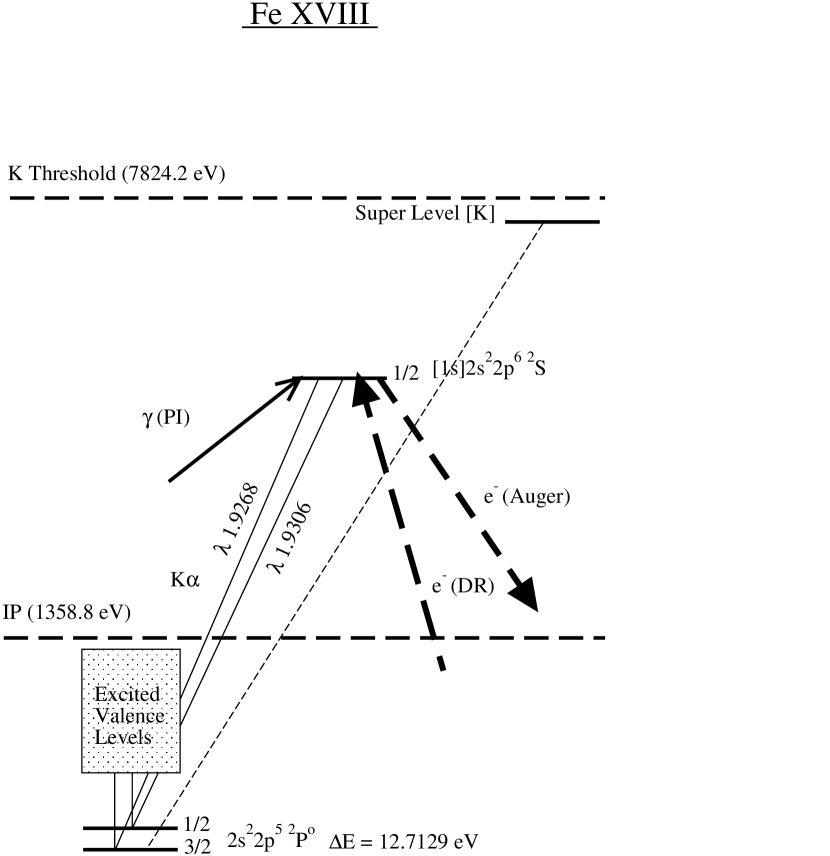
Figure 1.— Panel A: Simple Grotrian diagram for inner shell processes in Fe xviii

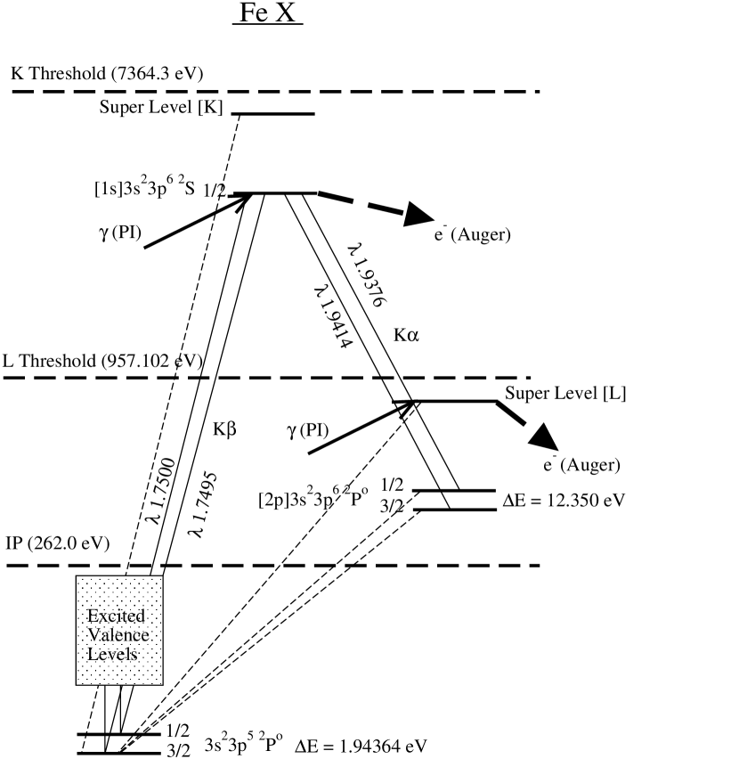
Figure 1.— Panel B: Simple Grotrian diagram for inner shell processes in Fe x

Figure 2.— K shell ionization thresholds (eV) vs. ionization state.

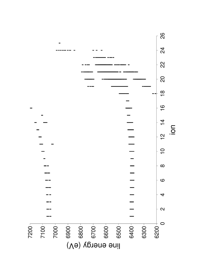
Figure 3.— K line energy (eV) vs. ionization state.

Figure 4.— Photoionization cross section in the K edge region vs. energy. Units of the cross section are cm^-2.

Figure 4.— continued

Figure 4.— continues

Figure 4.— continued

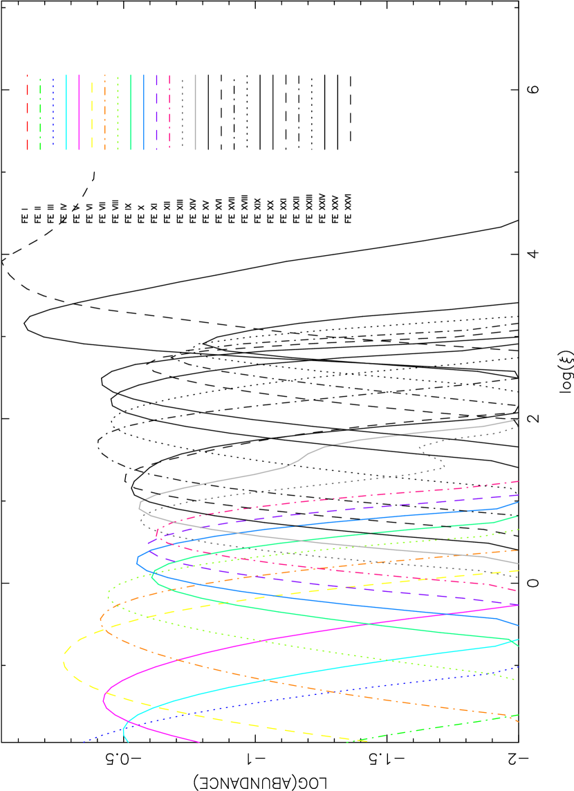
Figure 5.— Ion fractions vs. ionization parameter for iron. Based on an $F_{\varepsilon}\propto\varepsilon^{-1}$ ionizing continuum

Figure 6.— Temperature vs. ionization parameter for iron. Based on an $F_{\varepsilon}\propto\varepsilon^{-1}$ ionizing continuum

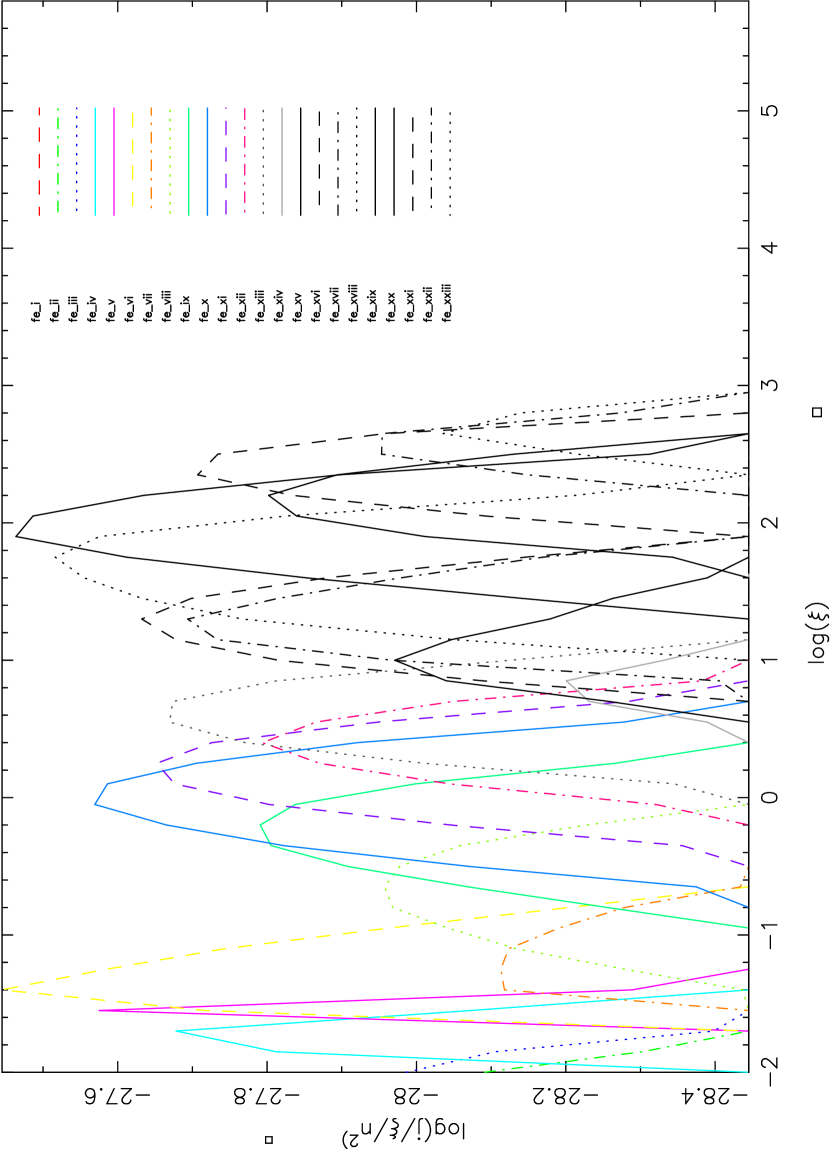
Figure 7.— Line emissivities per ion vs. ionization parameter for iron. For each ion, the emissivity of all K lines summed is plotted. Emissivity has been divided by ionization parameter for ease in plotting.

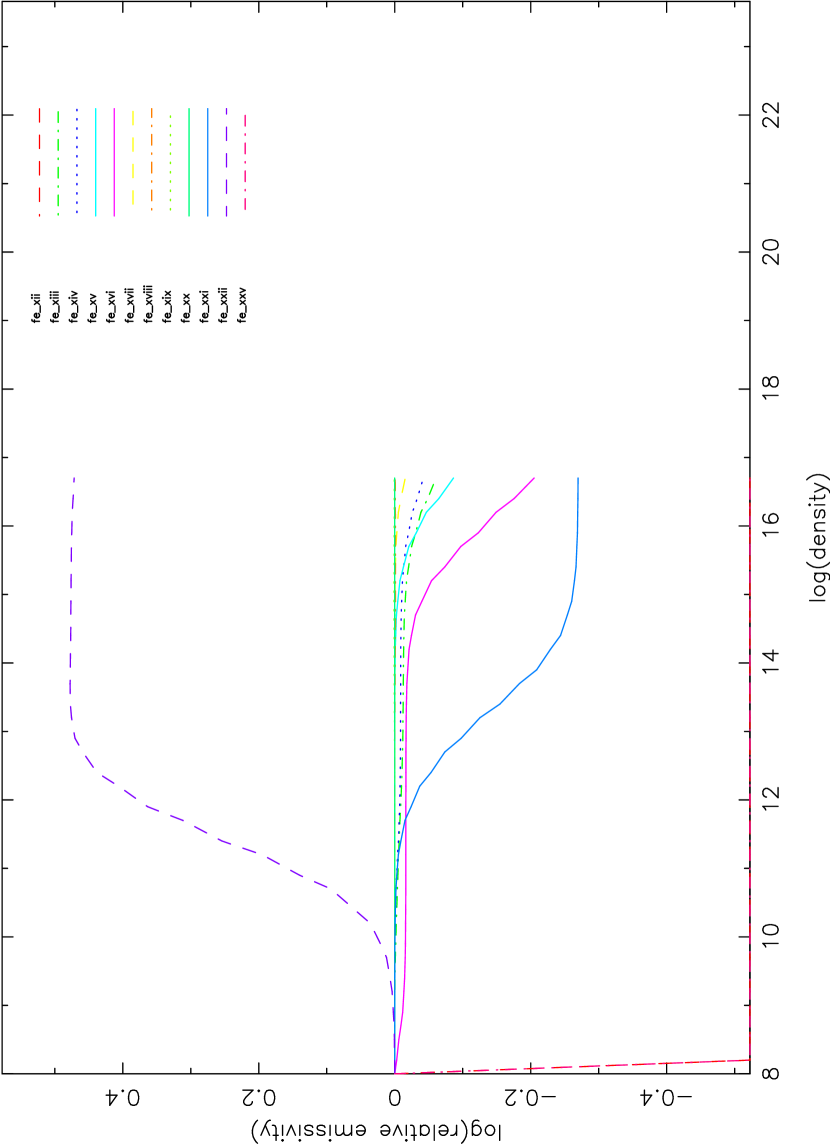
Figure 8.— Dependence of line emissivities on gas density. For each ion, the ratio of the emissivity of all K lines summed to the corresponding quantity at density 10⁸ cm^-3 is plotted.

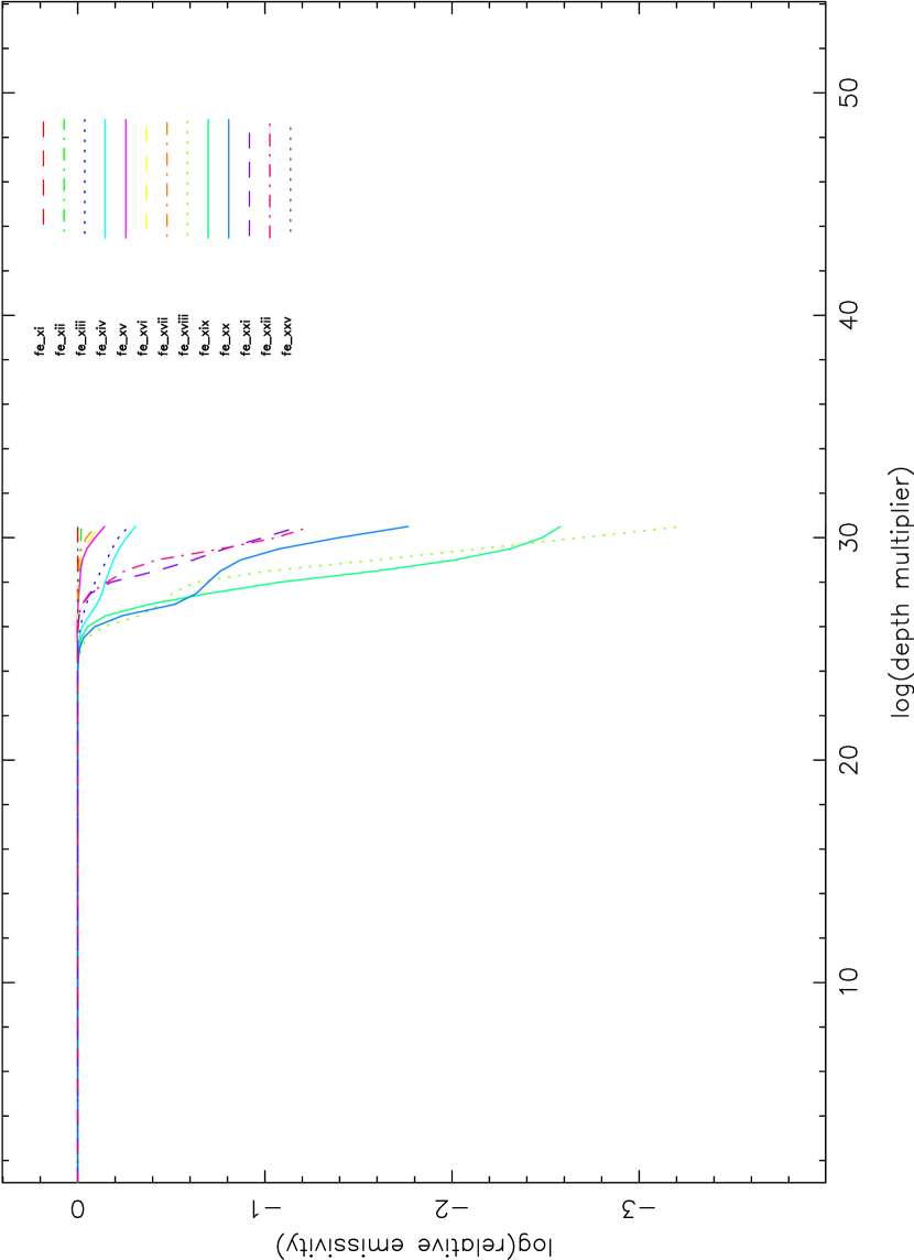
Figure 9.— Dependence of line emissivities on optical depth. As described in the text, the optical depth of each line calculated for a low-column slab is boosted by a depth multiplier. For each ion, the ratio of the emissivity of all K lines summed to the corresponding quantity when the depth multiplier is unity is plotted.

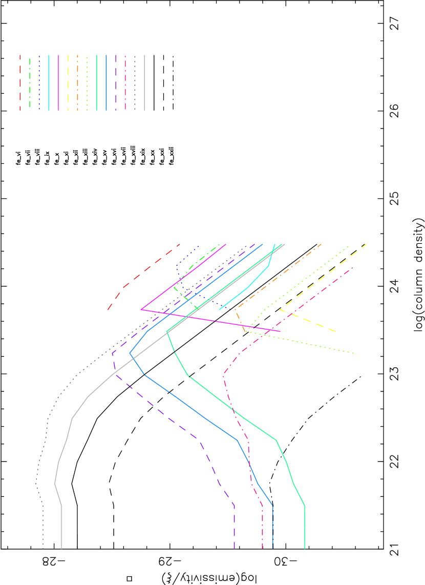
Figure 10.— Dependence of line emissivities on cloud column density. Units are the same as figure 7, averaged over the cloud volume.

Figure 11.— Emission line profiles for a family of thin (N=10¹⁷ cm^-2) slabs is plotted for various ionization parameter. Vertical scale is arbitrary, but is the same for all panels.

Figure 11.— continued

Figure 11.— continued

Figure 11.— continued

Figure 12.— Absorption spectra for a family of thick (N=3 $\times$ 10²³ cm^-2) slabs is plotted for various ionization parameter. Vertical scale is arbitrary, but is the same for all panels.

Figure 12.— continued

Figure 12.— continued

Figure 13.— Panel A: Simulated spectra of a 100 mCrab source with a spectrum similar to that shown in figure 12, log($\xi$)=2, log(N)=23, as observed with the PN instrument on XMM/Newton for 10⁵ seconds.

Figure 13.— Panel B: Simulated spectra of a 100 mCrab source with a spectrum similar to that shown in figure 12, log($\xi$)=2, log(N)=23, as observed with the XRS instrument on Astro-E2 for 10⁵ seconds.

Figure 13.— Panel C: Same as panel B, except using data from previous versions of xstar (v2.1d)

References

- Badnell (1997) Badnell, N. R. 1997, J. Phys. B, 30, 1
- Ballance et al. (2001) Ballance, C. P., Badnell, N. R., & Berrington, K. A. 2001, J. Phys. B, 34, 3287
- Bautista et al. (2003) Bautista, M. A, Mendoza, C., Kallman, T. R., & Palmeri, P. 2003, A&A, 403, 339 (Paper 1)
- Bautista et al. (2004) Bautista, M. A., Mendoza, C., Kallman, T. R., & Palmeri, P. 2004, A&A, 418, 1171 (Paper 6)
- Bautista et al. (1998) Bautista, M.A., Romano, P., & Pradhan, A.K. 1998, ApJS, 118, 259
- Beiersdorfer et al. (1989) Beiersdorfer, P., Bitter, M., von Goeler, S., & Hill, K. W. 1989, Phys. Rev. A, 40, 150
- Beiersdorfer et al. (1993) Beiersdorfer, P., Phillips, T., Jacobs, V. L., Hill, K. W., Bitter, M., von Goeler, S., & Kahn, S. M. 1993, ApJ, 409, 846
- Berrington & Ballance (2001) Berrington, K. A., & Ballance, C. 2001, J. Phys. B, 34, 2697
- Berrington et al. (1997) Berrington, K., Quigley, L., & Zhang, H. L. 1997, J. Phys. B, 30, 5409
- Burke & Seaton (1971) Burke, P. G., Seaton, M. J. 1971, Meth. Comp. Phys. 10, 1
- Chen (1986) Chen, M. H. 1986, At. Data Nucl. Data Tables, 34, 301
- Cowan (1981) Cowan, R. D. 1981, The Theory of Atomic Structure and Spectra (Berkeley, CA: University of California Press)
- Decaux & Beiersdorfer (1993) Decaux, V., & Beiersdorfer, P. 1993, Phys. Scr, T47, 80
- Decaux et al. (1997) Decaux, V., Beiersdorfer, P., Kahn, S. M., & Jacobs, V. L. 1997, ApJ, 482, 1076
- Decaux et al. (1995) Decaux, V., Beiersdorfer, P., Osterheld, A., Chen, M., & Kahn, S. M. 1995, ApJ, 443, 464
- Donnelly et al. (2000) Donnelly, D. W., Bell, K. L., Scott, M. P., & Keenan, F. P. 2000, ApJ, 531, 1168
- Gorczyca & Badnell (2000) Gorczyca, T. W., & Badnell, N. R. 2000, J. Phys. B, 33, 2511
- Grevesse & Sauval (1998) Grevesse, N., & Sauval, A., 1998, Space Sci. Rev., 85, 161
- House (1969) House, L. 1969, ApJS, 18, 21
- Jacobs & Rozsnyai (1986) Jacobs, V. L., & Rozsnyai, B. F. 1986, Phys. Rev. A, 34, 216
- Jacobs et al. (1980) Jacobs, V. L., Davis, J., Rozsnyai, B. F., Balazs, F., & Cooper, J. W. 1980, Phys. Rev. A, 21, 1917
- Jacobs et al. (1989) Jacobs, V. L., Doschek, G. A., Seely, J. F., & Cowan, R. D. 1989, Phys. Rev. A, 39, 2411
- Kaastra & Mewe (1993) Kaastra, J.S., & Mewe, R. 1993, A&AS, 97, 443
- Kallman & Bautista (2001) Kallman, T., & Bautista, M., 2001, ApJS, 133, 221
- Kato et al. (1997) Kato, T., Safronova, U. I., Shlyaptseva, A. S., Cornille, M., Dubau, J., & Nilsen, J. 1997, At. Data Nucl. Data Tables, 67, 225
- Liedahl (2003) Liedahl, D., 2003, in Atomic Data for X-Ray Astronomy, 25th Meeting of the IAU, Joint Discussion 17
- Makishima (1986) Makishima, K. 1986, in The Physics of Accretion onto Compact Objects, ed. K. P. Mason, M. G. Watson & N. E. White, Lecture Notes in Physics, 266 (Berlin: Springer-Verlag) 249
- Mendoza et al. (2004) Mendoza, Kallman, T. R., Bautista M. A., & Palmeri, P. 2004, A&A, 414, 377 (Paper 3)
- Palmeri et al. (2001) Palmeri, P., Quinet, P., Zitane, N., & Vaeck, N. 2001, J. Phys. B, 34, 4125
- Palmeri et al. (2002) Palmeri, P., Mendoza, C., Kallman, T. R., & Bautista, M. A. 2002, ApJ, 577, L119 (Paper 4)
- Palmeri et al. (2003a) Palmeri, P., Mendoza, C., Kallman, T. R., & Bautista, M. A. 2003a, A&A, 403, 1175 (Paper 2)
- Palmeri et al. (2003b) Palmeri, P., Mendoza, C., Kallman, T. R., Bautista, M. A., & Meléndez, M. 2003b, A&A, 410, 359 (Paper 5)
- Pravdo et al. (1977) Pravdo, S. H., Becker, R. H., Boldt, E. A., Holt, S. S., Serlemitsos, P. J., & Swank, J. H. 1977, ApJ, 215, L61
- Rau (1976) Rau, A. R. P. 1976, in Electron and Photon Interactions with Atoms, ed. H. Kleinpoppen & M. R. C. McDowell (New York: Plenum) 141
- Ross et al. (1996) Ross, R. R., Fabian, A. C., & Brandt, W. N. 1996, MNRAS, 278, 1082
- Sanford et al. (1975) Sanford, P., Mason, K. O., & Ives, J. 1975, MNRAS, 173, 9P
- Seely et al. (1986) Seely, J. F., Feldman, U., & Safronova, U. I. 1986, ApJ, 304, 838
- Serlemitsos et al. (1973) Serlemitsos, P. J., Boldt, E. A., Holt, S. S., Ramaty, R., & Brisken, A. F. 1973, ApJ, 184, L1
- Serlemitsos et al. (1977) Serlemitsos, P. J., Smith, B. W., Boldt, E. A., Holt, S. S., & Swank, J. H. 1977, ApJ, 211, L63
- Shirai et al. (2000) Shirai, T., Sugar, J., Musgrove, A., & Wiese, W. L. 2000, J. Phys. Chem. Ref. Data, Monograph 8
- Tanaka et al. (1995) Tanaka, Y., et al. 1995, Nature, 375, 659
- Verner and Yakovlev (1986) Verner, D., and Yakovlev, Y., 1986 Ap. J. Supp.
- Whiteford et al. (2002) Whiteford A. D., Badnell N. R., Ballance C. P., Loch, S. D., O’Mullane, M. G., & Summers, H. P. 2002, J. Phys. B, 35, 3729