Type Ia supernova rate at a redshift of $\sim$ 0.1

We present the type Ia rate measurement based on two EROS supernova search campaigns (in 1999 and 2000). Sixteen supernovae identified as type Ia were discovered. The measurement of the detection efficiency, using a Monte Carlo simulation, provides the type Ia supernova explosion rate at a redshift $\sim$ 0.13. The result is $0.125^{+0.044+0.028}_{-0.034-0.028}\ h_{70}^{2}$ SNu where 1 SNu = 1 SN / $10^{10}\ \textrm{L}_{\odot}^{B}$ / century. This value is compatible with the previous EROS measurement (Hardin et al. 2000), done with a much smaller sample, at a similar redshift. Comparison with other values at different redshifts suggests an evolution of the type Ia supernova rate.

1 Introduction

Type Ia supernovae are believed to be thermonuclear explosions of a white dwarf reaching the Chandrasekhar mass after accreting matter in a binary system (see e.g. Livio (2001)). They are the main mechanism to enrich the interstellar medium (ISM) with iron-peak elements (with $\sim$ 0.6 M_⊙ of nickel released per event on average). The knowledge of the number of such events per galaxy and per unit of time is crucial to understand the matter cycle and the ISM chemistry. From a cosmological point of view the measurement of the evolution of the explosion rate will put strong constraints on galaxy evolution. Measuring the evolution of the core-collapse supernovae (type II and Ib/c) explosion rate would give a new unbiased view on the star formation rate (SFR) history, independent of any peculiar tracer, because gravitational supernovae are directly linked to massive star formation. Up to now, the type II supernova rate has been measured only in the local Universe (Cappellaro et al. 1999). On the other hand, the measurement of the evolution of the explosion rate of type Ia supernova would give strong constraints on the SFR history and on many other parameters such as the progenitor evolution (birth rate of binaries, time delay between the white dwarf formation and the thermonuclear explosion…) or the nature of the progenitor itself.

This paper is organized as follows: first the EROS search for supernovae is reviewed in Sect. 2. Then the two supernova search campaigns at the origin of this work are presented in Sect. 3. Sections 4 to 7 deal with the rate computation. Our results are presented in Sect. 8 and discussed in Sect. 9.

2 The EROS search for supernovae

The EROS experiment used a 1-meter telescope based at La Silla observatory, Chile, designed for a baryonic dark matter search using the microlensing effect (see e.g.  Lasserre et al. 2000; Afonso et al. 2003b, a). The telescope beam light was split by a dichroic cube into two wide field cameras (1 deg²). The cube sets the passband of both cameras, a “blue” one overlapping the $V$ and $R$ standard bands, another “red” one matching roughly the $I$ standard band. Each camera was a mosaic of eight 2048 $\times$ 2048 pixels CCDs with a pixel size of $0.60^{\prime\prime}$ on the sky (Bauer & de Kat 1997; Palanque-Delabrouille et al. 1998). In the following, we will use only the blue camera. One “image” stands for one CCD, and one “field” is for the entire camera with its eight CCDs, i.e. $\sim$ 1 deg².

A wide field camera is a good asset to perform supernova searches as the number $n$ of detected supernovae is proportional to $\Omega\cdot z_{\text{lim}}^{2}$ where $\Omega$ is the solid angle surveyed and $z_{\text{lim}}$ is the limiting redshift of the search – typically EROS detected type Ia supernovae up to $z=0.3$. EROS dedicated about 15 % of its time to supernova search between 1997 and 2000. The main limitation has been to secure enough telescope time to perform the photometric and spectroscopic follow-up of discovered events.

To search for supernovae EROS uses the CCD subtraction technique which consists in observing the same fields three weeks to one month apart in order to detect transient events and catch only supernovae near maximum light (a typical type Ia supernova reaches its maximum light in the optical wavelength roughly 15 to 20 days after the explosion). Both observations are done around new moon in order to limit the sky background. The two sets of images are then automatically subtracted after a spatial alignment, a flux alignment and a seeing convolution.

Cuts are applied to eliminate known classes of variable objects such as asteroids, variable stars, and cosmic rays. The most important cut is the requirement that the transient object be near an identified galaxy. More precisely, it is required to be within an ellipse centered on any galaxy with semi-major and minor axes of length 8 times the r.m.s. radius of the galaxy’s flux distribution along each axis. This ellipse should contain essentially all supernovae associated with a galaxy since $\sim 99$ % of galactic light is contained within an ellipse of size 3 times the r.m.s. radius. To eliminate cosmic rays, each exposure consists in two subexposures: SExtractor (Bertin & Arnouts 1996) software is run on both images to make a cosmic-ray catalog before adding the two images.

In spite of these cuts, a human eye is still needed to check the remaining candidates and discard obvious artefacts (residual cosmic rays, bad subtractions, asteroids, variable stars…). Ten to fifteen search fields are observed every night and the human scanner has to deal with about 100 candidates the following day. The serious candidates are observed again on the following night for confirmation. Then a spectrum is taken to obtain the supernova type, phase and redshift.

EROS supernova search fields lay near the celestial equator (declination between $-4.5^{\circ}$ and $-12^{\circ}$) to be reached from both hemispheres and between 10${}^{\text{h}}$ and 14.5${}^{\text{h}}$ in right ascension. They overlap some of the Las Campanas Redshift Survey (LCRS) (Shectman et al. 1996) fields which will facilitate the galaxy sample calibration.

3 The 1999 and 2000 campaigns

IAU Name	Date (UT)	$\boldsymbol{V}$	$\boldsymbol{\alpha_{J2000.0}}$	$\boldsymbol{\delta_{J2000.0}}$	z	Type	Phase (days)	IAUC
SN 1999ae	1999-02-10	20.7	11 51 24.48	-04 39 09.4	0.076	II	$<+30$	7117
SN 1999af	1999-02-12	19.2	13 44 50.95	-06 40 12.6	0.097	Ia	$-10$	7117
SN 1999ag	1999-02-12	20.1	12 15 22.81	-05 18 12.4	0.099	II		7117
SN 1999ah	1999-02-13	20.5	12 09 37.20	-06 18 34.3	0.080	SN?		7117-18
SN 1999ai	1999-02-15	18.0	13 14 10.57	-05 35 43.7	0.018	II	$\sim$ +14	7117-18
SN 1999aj	1999-02-17	20.9	11 22 39.34	-11 43 53.9	0.186	Ia		7117
SN 1999ak	1999-02-17	18.5	11 06 52.05	-11 39 13.3	0.055	Ia	$\sim$ +14	7117-18
SN 1999al	1999-02-21	19.2	11 10 25.68	-07 26 37.0	0.065	Ic	-9	7117-18
SN 1999bi	1999-03-10	19.8	11 01 15.76	-11 45 15.2	0.124	Ia	+2	7136
SN 1999bj	1999-03-10	20.5	11 51 38.39	-12 29 08.3	0.16	Ia	+17	7136
SN 1999bk	1999-03-14	18.9	11 28 52.01	-12 18 08.3	0.096	Ia	+1	7136
SN 1999bl	1999-03-14	20.7	11 12 13.60	-05 04 44.8	0.300	Ia	0	7136
SN 1999bm	1999-03-17	20.0	12 45 00.84	-06 27 30.2	0.143	Ia	-1	7136
SN 1999bn	1999-03-16	19.6	11 57 00.40	-11 26 38.4	0.129	Ia	-5	7136
SN 1999bo	1999-03-17	19.5	12 41 07.48	-05 57 25.8	0.130	Ia	$>0$	7136
SN 1999bp	1999-03-19	18.6	11 39 46.42	-08 51 34.8	0.077	Ia	-4	7136
SN 1999bq	1999-03-19	20.7	13 06 54.46	-12 37 11.6	0.149	Ia	-1	7136
SN 2000bt	2000-03-26	19.4	10 16 18.05	-05 44 47.3	0.04	Ia	+20	7406
SN 2000bu	2000-03-31	19.4	11 27 11.45	-06 23 14.6	0.05	II?	$\sim$ 0	7406
SN 2000bv	2000-04-01	20.6	12 59 28.70	-12 20 07.6	0.12	II?	$\sim$ 0	7406
SN 2000bw	2000-04-04	20.5	11 09 49.85	-04 24 46.4	0.12	II?	$\sim$ 0	7406
SN 2000bx	2000-04-06	19.2	13 48 55.55	-06 18 35.9	0.09	Ia	$\sim$ 0	7406
SN 2000by	2000-04-07	19.2	11 39 54.91	-04 22 16.4	0.10	Ia	$\sim$ 0	7406
SN 2000bz	2000-04-08	21.2	14 15 02.66	-06 17 16.0	0.26	Ia	$\sim$ 0	7406

Table 1: List of supernovae discovered by EROS in 1999 and 2000. From left to right: IAU name of each event, discovery date, discovery $V$ magnitude, SNe celestial coordinates, redshift, type, phase (discovery time from maximum light) and IAU.

At the beginning of 1999, the Supernova Cosmology Project (SCP) undertook a large nearby supernova search involving eight supernova search groups, including EROS. The goal was to gather a large set of well sampled, CCD discovered, nearby ($z\lesssim 0.15$) type Ia supernovae in order to calibrate the distant events used to measure the cosmological parameters. The whole collaboration obtained 37 SNe out of which 19 were type Ia SNe near or before maximum light and were followed both spectroscopically and photometrically. EROS observed 428 square degrees of sky in two steps and discovered 12 type Ia (cf. IAUC 7117 and 7136) of which 7 have been followed by the collaboration. After obtaining reference images of search fields in January 1999 (01/12 to 01/29), the SN search was conducted between February 4 and February 27 (new moon was on February 16), and between March 09 and March 27 (new moon was on March 17).

One year later, EROS was involved with the European Supernova Cosmology Consortium (ESCC, involving French, British, Swedish and Spanish institutes) to search for intermediate redshift ($z\sim 0.2-0.4$) supernovae. Four type Ia supernovae were discovered (cf. IAUC 7406). One hundred and seventy square degrees were observed between 2000, March 27 and April 9 (new moon on April 4); reference images were taken between February 27 and March 15. The main difference between the two searches was the exposure time used: for the 1999 campaign it was set to 300 seconds, while for the 2000 search it was 600 seconds allowing a deeper search by 19 % in redshift (as $z_{\text{lim}}\propto T_{\text{exp}}^{1/4}$, where $T_{\text{exp}}$ the exposure time).

In both campaigns, spectra of each candidate were taken. The main characteristics of the discovered supernovae are summarized in Table 1.

4 Principle of the measurement

Our supernovae search requires that a supernova be associated with an identified host galaxy. We must therefore make an assumption about how the supernova rate scales with galaxy luminosity, so as to correct the rate for supernovae in dim, unidentified galaxies. We choose to assume that the number of supernovae per galxay and per unit time is proportional to the red galaxy luminosity, an assumption that receives some empirical support, though mostly in the blue band (Tammann 1970; Cappellaro et al. 1993). Under this assumption, the explosion rate $\mathcal{R}_{\text{SN}}$ is given by the ratio of the number of detected supernovae of type Ia $\mathcal{N}_{\text{SNe}}$, to the number of galaxies to which the search is sensitive $\mathcal{N}_{\text{gal}}$, weighted by their mean luminosity $\langle\mathcal{L}_{\text{gal}}\rangle$ and by the mean time interval $\langle\mathcal{T}\rangle$ during which the supernovae can be detected:

$$\mathcal{R}_{\text{SN}}=\frac{\mathcal{N}_{\text{SNe}}}{\mathcal{N}_{\text{gal}}\cdot\langle\mathcal{L}_{\text{gal}}\rangle\cdot\langle\mathcal{T}\rangle}.$$ (1)

The time interval or control time $\mathcal{T}$ during which a given supernova is visible depends on the supernova detection efficiency $\varepsilon$. Since the efficiency itself depends on many parameters, the observed control time $\mathcal{T}$ for a supernova of redshift $z$ is given by an integral of $\varepsilon$ over these parameters:

$$\mathcal{T}(z)=\int_{\phi_{\text{SNIa}}}\int^{+\infty}_{-\infty}\varepsilon(\Delta;m(t,z;\phi_{\text{SNIa}}))\ dt\ d\phi_{\text{SNIa}},$$ (2)

where $\Delta$ is the time interval between the search images and the reference images; $m(t,z;\phi_{\text{SNIa}})$ is the supernova apparent magnitude ($t$ is the time from maximum light or phase; $z$ is the redshift). The magnitude $m$ depends also indirectly on the light curve distribution of type Ia supernova (see § 7.3), that we note $\phi_{\text{SNIa}}$. As we know the galaxy sample in the search images (see § 5), but not their redshifts, the restframe explosion rate can be rewritten as:

$$\mathcal{R}_{\text{SN}}=\frac{\mathcal{N}_{\text{SNe}}}{\sum_{g}\int_{0}^{+\infty}p(z|m_{g})\cdot\mathcal{L}_{g}(m_{g},z)\cdot\mathcal{T}(z)/(1+z)\cdot dz},$$ (3)

where $g$ is a subscript running on all galaxies of all the search images; $p(z|m_{g})$ is the probability density of the redshift $z$ of a galaxy knowing its apparent magnitude $m_{g}$ (see § 7.2); $\mathcal{L}_{g}$ is the galaxy luminosity (which depends on its redshift and apparent magnitude, as well as on a cosmological model: we use a standard model, ($\Omega_{M_{\circ}},\,\Omega_{\Lambda_{\circ}}$) = (0.3, 0.7); for the Hubble constant, we use the notation $H_{\circ}\leavevmode\nobreak\ =\leavevmode\nobreak\ 70\ h_{70}\ \text{km}\ \text{s}^{-1}\ \text{Mpc}^{-1}$ wherever needed). Different steps are needed to calculate the denominator of eq. (3). The first one is to establish a well-defined sample of galaxies in the search images. This is then used to measure the detection efficiency. Each of these steps is detailed in the following sections.

In the following the EROS instrumental magnitude will be denoted:

$$\widetilde{\mathcal{B}}_{\text{eros}}\equiv-2.5\cdot\log\frac{\mathcal{F}_{ADU}}{T_{\text{exp}}}$$ (4)

where $\mathcal{F}_{ADU}$ is the flux as measured in CCD images in digital units; $T_{\text{exp}}$ is the exposure time in seconds. Throughout this paper the magnitudes in EROS images are computed using an adaptive aperture photometry as provided by the SExtractor software (Bertin & Arnouts 1996), which is accurate enough for our purpose. Photometry for stellar objects was done using observations of Landolt stars, as detailed in Sect. 7.4. Galactic magnitudes needed to derive the redshift distribution and to normalize the SN rate was calibrated using LCRS $R$ magnitudes.

5 The galaxy sample

We use the SExtractor software (Bertin & Arnouts 1996) to detect objects on the images. Objects are classified as stars and galaxies using the SExtractor CSTAR parameter which quantify the “stellarness” of an object. For stars CSTAR $\rightarrow$ 1, and for galaxies CSTAR $\rightarrow$ 0. The critical input in order to obtain a reliable value of this parameter is the image seeing. SExtractor is then run twice on the images, first to obtain the seeing, and a second time to compute CSTAR. Figure 1 shows a scatter plot of CSTAR versus the galaxy magnitude. We see that the galaxy star separation is clear for $R<19$. The galaxies of the LCRS catalog (Shectman et al. 1996) shown in the plot allow one to verify the efficiency of the classification for $R<18$.

Figure 1: EROS magnitude distribution vs. value of CSTAR. Objects with CSTAR around 0.5 are faint and thus difficult to classify. Squares stand for LCRS galaxies. The dark line represents the cut (5) for the 1999 search.

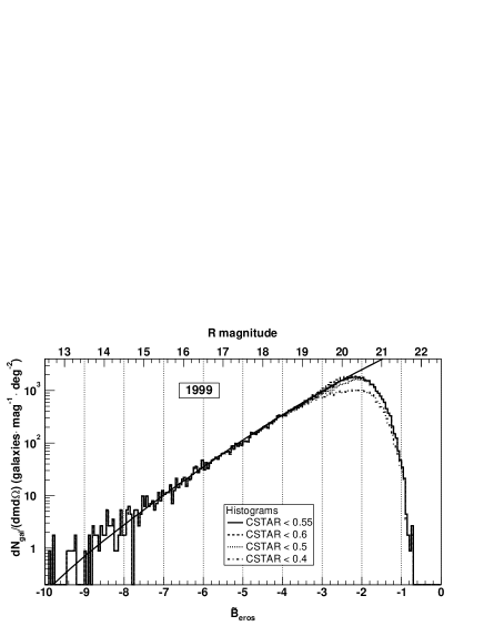
(a) Galaxy count on EROS fields done on 180 images from the 1999 search. The completeness limit is for CSTAR $<$ 0.55 and $\widetilde{\mathcal{B}}_{\text{eros}}<-2.6$.

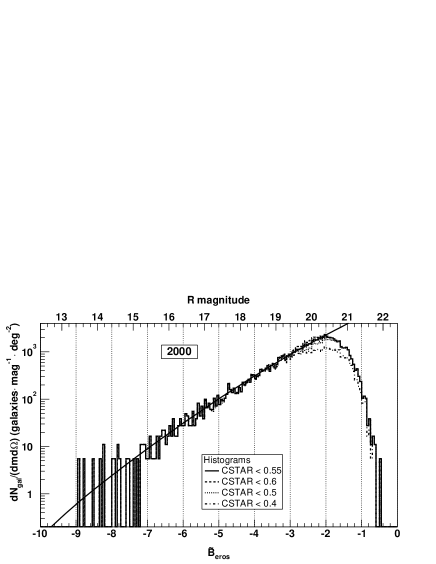
(b) Galaxy count on EROS fields done on 29 images from the 2000 search. The completeness limit is for CSTAR $<$ 0.55 and $\widetilde{\mathcal{B}}_{\text{eros}}<-2.2$.

Figure 2: Galaxy counts in EROS supernova fields for various cuts on the CSTAR parameter. The nominal value for this cut is CSTAR $<$ 0.55. Beyond, faint stars pollute the galaxy sample. Below, faint galaxies are missed. The curve stands for published data such as the count in $R$ band by Bertin & Dennefeld (1997). The matching of the curve with the histogram confirms our galaxy magnitude calibration, eq. (13). The main difference between the 1999 and the 2000 searches was the exposure time, set to 300 seconds in 1999 and 600 seconds in 2000.

To further check the reliability of the galaxy sample we make a “galaxy count” that we compare to published ones. As illustrated in Fig. 2 we are able to define accurately the completeness limit of our survey as the point where our data turn down relative to the published counts. At this point, stars and galaxies are quite hard to distinguish: most of the objects still have a CSTAR $\sim$ 0.5 (see Fig. 1 for $\widetilde{\mathcal{B}}_{\text{eros}}\sim-2.6$). To take this into account, we set the galaxy magnitude cut one magnitude below the completeness limit in order to prevent contamination of our galaxy sample by stars. Then:

$$\text{for}\ 1999\ \left\{\begin{array}[]{l}\text{CSTAR}<0.55,\\ \widetilde{\mathcal{B}}_{\text{eros}}<-3.5;\ (\textit{i.e.}\ R<19),\\ \end{array}\right.$$ (5)

$$\text{for}\ 2000\ \left\{\begin{array}[]{l}\text{CSTAR}<0.55,\\ \widetilde{\mathcal{B}}_{\text{eros}}<-3.1;\ (\textit{i.e.}\ R<19.3).\\ \end{array}\right.$$ (6)

The effect of this cut is shown in Fig. 1. We used the LCRS galaxy catalog (Shectman et al. 1996) to check it, as illustrated in Fig. 1. This cut removes events in faint galaxies which are visually indistinguishable from variable stars.

According to the LCRS luminosity function (Lin et al. 1996), our cut requiring $R<19$ means that at our mean redshift of 0.13 (see Fig. 11), our supernova search is sensitive to supernovae in galaxies that generate about 85 % of the total stellar luminosity. We are not sensitive to supernovae in the multitude of low-luminosity galaxies but these galaxies generate little total light. If the supernova rate is proportional to the luminosity, they also generate few supernovae.

6 The detection efficiency

In order to measure the detection efficiency, we superimpose simulated supernovae on the galaxies. On each search image we choose a bright – but not saturated – star (with a signal to noise ratio typically above 50) as a template to be “copied” onto the potential host galaxy. Among all such stars found in the image, we take the one nearest to the galaxy on which we wish to add a supernova. We move only the pixels included in a circle with a radius given by the point where the star flux calculated by using a gaussian is equal to half a standard deviation of the sky background. Each pixel is rescaled to the desired flux (simulated supernova flux is distributed uniformly between 0 and 15 000 ADU – the latter corresponding roughly to $V\sim 18.5$ for 1999 and to $V\sim 19.2$ for 2000). Simulated supernovae are placed at random positions within the isophotal limits of the galaxy, i.e. inside an ellipse centered on the galaxy and that has semi-major and minor axes of length 3 times the r.m.s. of the galaxy’s flux along the axis distribution; this ellipse contains $\sim$99 % of the galaxy flux. The positions are chosen following a probability proportional to the local surface brightness. They are placed on the galaxies of the images before the search software is run. A simulated supernova is detected by the search software if its signal-to-noise ratio is greater than 5 and if it is situated within a radius of 1.5 pixels of the simulated one, according to Fig. 3. The resulting efficiency as a function of the simulated SN flux is the ratio between detected supernovae and simulated ones. The result is fitted by an analytic function in order to smooth the histogram. The efficiency used in eq. (2) is computed for each search image. A “global” efficiency computed for each of the two campaigns as a function of simulated flux is shown in Fig. 4 with the resulting fits. Figure 5 shows this “global” efficiency as a function the simulated SN distances to their hosts. We remark that we observe no significant efficiency loss in the center of galaxies. This improvement comes from using CCD detectors instead of photographic plates (where the core of galaxies saturates – see e.g. Howell et al. (2000)). Moreover the efficiency is roughly independent of the position within the central $\sim 8^{\prime\prime}$ of the galaxies. Beyond this radius, corresponding to the isophotal limit of most galaxies in our sample, few supernovae are simulated leading to the large statistical fluctuations in Fig. 5. Near the center of galaxies, the efficiency is about 0.9, limited mostly by “geometrical” losses near CCD edges and around dead pixels.

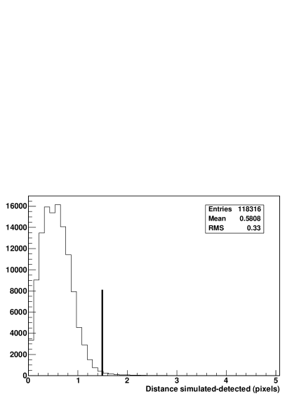
Figure 3: Histogram of the distance between the simulated supernovae and the detected ones. The cut we used to identify the detected population is set at a radius of 1.5 pixels from the simulated supernova as shown by the dark line.

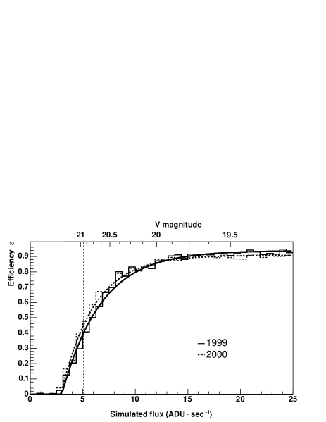
Figure 4: Mean efficiency computed for each of the two searches as a function of the simulated flux, in ADU s^-1 or $V$ magnitude (according to eq. (12)), for both the 1999 search (continuous line) and the one of 2000 (dashed line). The curves are the fits. With its exposure time twice the one of 1999, the 2000 search went about 0.2 mag deeper. The two vertical lines represent the limiting magnitudes defined as the magnitude at half the maximum efficiency: 5.59 ADU s^-1 for 1999 and 5.09 ADU s^-1 for 2000. The ratio between the two limits is 1.10, to be compared with 1.41 expected for an exposure time ratio of 2. The plateaux reached at high flux are respectively 0.94 and 0.91 for 1999 and 2000.

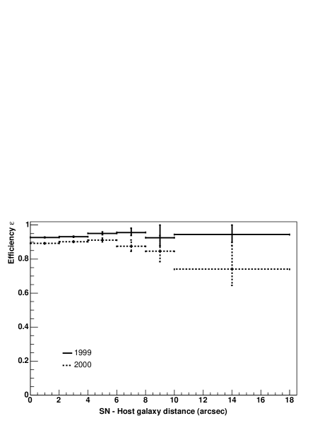
Figure 5: Mean efficiency as a function of the distance of simulated supernovae to their host galaxy peaks, computed for each of the two searches. Since there is a loss of efficiency at low fluxes, this plot is done for fluxes above 20 ADU s^-1 for 1999 and above 13 ADU s^-1 for 2000.

7 The integral computation

7.1 The algorithm

To compute the integral in the denominator of eq. (3), we have to integrate the detection efficiency over various parameters, such as the type Ia supernova light curve distribution, the supernova redshift and its phase at the time of discovery (time from maximum light). In order to do that, we use a Monte-Carlo method: a light curve is randomly drawn among a selected set of SNe (see Sect. 7.3); a redshift is drawn according to the probability density $p(z|m_{g})$ as defined in Sect. 7.2; the selected light curve is adjusted according to this redshift. A phase is drawn uniformly, which provides a standard magnitude. After transformation of standard $V$ and $R$ magnitudes into ADU (see Sect. 7.4), the corresponding efficiency is read from Fig. 4.

Figure 6: Examples of redshift distributions of galaxies knowing their apparent magnitude, as given by (7). The solid lines show the predicted distribution for three apparent magnitudes $m_{g}$ and two sets of cosmological parameters. The histograms show the distribution of LCRS redshifts for galaxies within 0.1 mag of the given magnitude.

7.2 Redshift distribution of galaxies

We do not know the redshifts of all the galaxies in the images. But all we need is the probability distribution $p$ for the redshift $z$ given the galaxy’s apparent magnitude $m_{g}$:

$$p(z|m_{g})\varpropto\frac{dN}{dm_{g}dzd\Omega}=\frac{dV_{c}}{d\Omega dz}\cdot\phi_{g}(M_{g})$$ (7)

where $N$ is the number of galaxies having this redshift and apparent magnitude, $\Omega$ is the solid angle surveyed, $V_{c}$ is the comoving volume and $\phi_{g}$ the galaxy luminosity function ($M_{g}$ being their absolute magnitude). To compute this, we use the luminosity function of the LCRS (Lin et al. 1996). Figure 6 gives examples of such a distribution.

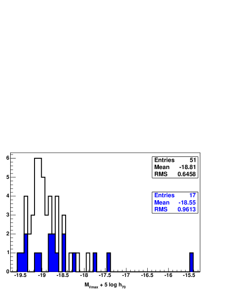
Figure 7: Absolute $V$ magnitude at maximum light distribution for the whole published set (51 SNe, white histogram, upper box) and the reference sample of 17 supernovae we selected (blue histogram, lower box). If we remove the lowest luminosity event (SN 1996ai) from this reference sample, its mean is shifted from $-$18.55 to $-$18.75.

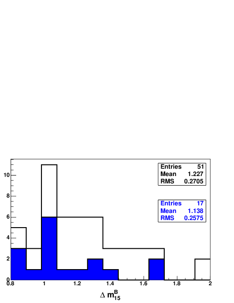
Figure 8: Distribution of the light curve shape parameter $\Delta m_{15}^{B}$ for the whole published set (51 SNe, white histogram, upper box) and the reference sample of 17 supernovae we selected (blue histogram, lower box).

7.3 Type Ia supernova light curve distribution

We need to integrate the efficiency on a large and representative sample of supernova light curves, so as to reproduce the variety of such objects. The light curve distribution of type Ia supernova can be parametrized, at least at first order, using two parameters: the luminosity at maximum light, and a light curve shape parameter. The light curve shape can be quantified using the $\Delta m_{15}^{B}$ parameter (Phillips 1993), that is the magnitude difference between the light at maximum and 15 days later on the $B$ light curve.

Out of 51 published type Ia supernovae observed light curves (Hamuy et al. 1996; Riess et al. 1999), we selected a reference sample of seventeen objects that have a good sampling in both $V$ and $R$ bands, the standard bands used to calibrate the EROS band. Each light curve is then fitted with an analytic template (Contardo et al. 2000), which allows us to reach any point of the light curve without interpolation; the selected objects of the reference sample have a very good fit. The resulting distribution of absolute magnitude at maximum light (the luminosity function) is shown in Fig. 7. The reference sample we have used has a lower mean luminosity than the full sample. This is mainly due to one very subluminous event, SN 1996ai (which may be very extinguished by its host galaxy – $A_{V}\sim 4$ according to Tonry et al. (2003)). The $\Delta m_{15}^{B}$ distribution of the reference sample is shown in Fig. 8; it is similar to that of the full sample. Our supernova rate will be presented in a form such that it can be revised if future measurements give different values for the mean luminosities and $\Delta m_{15}^{B}$.

7.4 From standard magnitudes to ADUs

As the detection efficiency is measured as a function of supernova flux in the EROS band, and as the published light curve sample we will use to reproduce the supernova light curve distribution is expressed in standard magnitudes, we need to translate one system into the other using a calibration relation such as:

$$\widetilde{\mathcal{B}}_{\text{eros}}=V+\alpha\cdot(V-R)+\beta+\delta\cdot(\xi-1),$$ (8)

between the measured flux on the CCD images ($\widetilde{\mathcal{B}}_{\text{eros}}$ is defined by eq. (4)) and the observed magnitudes through the standard bands: we choose $V$ and $R$ which are the closest to the EROS band; $\alpha$ is the color term; $\beta$ is the so-called zero point; $\delta\cdot(\xi-1)$ ($\xi$ is the airmass) is the atmospheric absorption: the atmospheric absorption at meridian (i.e. at $\sim 20^{\circ}$ from the zenith) is included in the zero point. $V$ and $R$ are related to the intrinsic magnitudes of the supernova $V_{sn}$ and $R_{sn}$ after correcting for the various extinctions:

$$V=V_{sn}+A_{V}+A_{V}^{\text{extra}},$$ (9)

$$R=R_{sn}+A_{R}+A_{R}^{\text{extra}},$$ (10)

where $A_{V}$ and $A_{R}$ are the Galactic absorption; $A_{V}^{\text{extra}}$ and $A_{R}^{\text{extra}}$ are the extragalactic absorption which could be either an intergalactic extinction or a host galaxy extinction or both.

Moreover, we use light curves of observed nearby supernovae. These light curves are transformed to any redshift; the relationship between the published light curve $m_{F}(t_{1},z_{1})$ in a filter $F$ and the “new” redshifted light curve $m_{F}(t_{2},z_{2})$ is given by

$$\begin{split}m_{F}(t_{2},z_{2})-&m_{F}(t_{1},z_{1})=5\log\frac{\mathcal{D}(z_{2})}{\mathcal{D}(z_{1})}\\ &\quad+K_{F}(t_{2},z_{2})-K_{F}(t_{1},z_{1}),\\ \end{split}$$ (11)

where $\mathcal{D}$ is the luminosity distance and $K$ is a term which takes into account the fact that we observe objects whose flux is sliding according to their redshift through a fixed passband in wavelength space. This term is known as the “$K$-correction” (see Sect. 7.4.5). Note that this relation does not depend on the Hubble constant. The following sub-sections deal with the different terms described above.

7.4.1 Can we calibrate supernovae using stars?

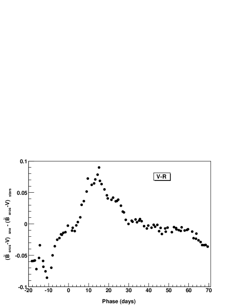
Figure 9: Evolution with the supernova phase of the error we made when using stars to calibrate supernovae. What is actually plotted is the difference between zero points computed for SNe Ia $(\widetilde{\mathcal{B}}_{\text{eros}}-V)_{\text{sne}}$ and for stars $(\widetilde{\mathcal{B}}_{\text{eros}}-V)_{\text{stars}}$. Each dot stands for a star whose color $(V-R)$ is equal to the $(V-R)$ color of a SNIa at that phase. The signal difference is never larger than 8 %. The colors are computed from template spectra.

As SN spectra are very different from star spectra, showing broad blended features evolving along the SN phase, we may wonder to what extent we can use stars to calibrate SN fluxes. In order to quantify this effect, we use synthetic colors computed with template spectra for each phase of the SN. Figure 9 shows the error we make when calibrating type Ia supernova fluxes using stars, as a function of the supernova phase. Assuming the color is the same for SNe and stars ($\alpha_{\text{SNe}}\approx\alpha_{\text{stars}}$), the plotted quantity $(\widetilde{\mathcal{B}}_{\text{eros}}-V)_{\text{sne}}-(\widetilde{\mathcal{B}}_{\text{eros}}-V)_{\text{stars}}$ reflects directly the zero point differences, $\beta_{\text{SNe}}-\beta_{\text{stars}}$. The error is at most 8 % around $-$10 days and between +10 and +20 days. We note that for standard filters, there would be no such error.

7.4.2 Zero point and color term for the stars

(a) Zoom on the 1999 supernova search: the mean zero point is about 22.7 during the supernova search (see first box for the February campaign, and second box for the March campaign).

(b) Zoom on the 2000 supernova search: the mean zero point is 5 % lower than the one from 1999 searches (see box).

Figure 10: Evolution of the “blue” zero point as a function of time. Circles stand for the calibration using the Landolt catalog; black filled circles are for secondary calibrating stars from the supernova calibration of SCP 1999 set; crosses are absorption coefficients from EROS analysis of LMC and SMC stars, shifted to match the Landolt points. The February 1999 search has been done between 02/04 and 02/27; the March 1999 search was performed between 03/09 and 03/27; The April 2000 search took place between 03/27 and 04/09. For these three campaigns the corresponding zero point is 22.7 within a 5 % range. The total uncertainty on this measurement is, from the scatter of the points, about $\pm$7 %.

Zero points for the EROS observations are computed from standard stars (Landolt 1992) or secondary standard stars around some EROS supernovae which were followed-up and analyzed by the SCP (Regnault et al. 2001). As the observations were always done close to the meridian, the atmospheric absorption correction is included in the zero point. The evolution of the zero point as a function of time is plotted in Fig. 10. Within a 5 % accuracy, it is the same for the 1999 and the 2000 searches. The color term is computed using the SMC and LMC OGLE calibrated catalog (Udalski et al. 2000) in order to have a larger lever arm: the Landolt catalog has the drawback to have mainly red (87 % have $B-V\gtrsim 0.3$) stars. This can be overcome with the OGLE catalog of SMC and LMC stars, that EROS is surveying too in its microlensing search program. The result is

$$\widetilde{\mathcal{B}}_{\text{eros}}=V-0.53\cdot(V-R)-22.7.$$ (12)

The zero point above is obtained for one CCD of the EROS mosaic, the seven other CCDs (that have different gains) are calibrated relative to this one, using the sky background and various photometric catalogs. The relative variation from CCD to CCD is of order of 10 %.

7.4.3 Zero point for the galaxies

To calibrate the galaxy magnitudes we use the LCRS catalog which provides a single isophotal $R_{\text{lcrs}}$ magnitude (Lin et al. 1996). We find:

$$\widetilde{\mathcal{B}}_{\text{eros}}=R_{\text{lcrs}}-22.7.$$ (13)

Lin et al. (1996) estimate that $R=R_{\text{lcrs}}-0.25$. The distribution of $\widetilde{\mathcal{B}}_{\text{eros}}-R_{\text{lcrs}}$ for the LCRS galaxies has a r.m.s. width less than 0.2 mag. This width is sufficiently narrow that it was not necessary to refine eq. (13) with a color term. The reason that little precision is necessary is that the galaxy magnitudes are only used, first, to derive the redshift probability distribution for each galaxy and, second, to calculate the total galactic luminosity of the sample to normalize the supernova rate. In both cases, one effectively averages over all galaxies in the sample so the relation (13) is sufficiently accurate.

7.4.4 Extinction

Observations are always performed close to the meridian, so the resulting atmospheric absorption can be considered constant and included in the zero point.

The Galactic extinction is corrected field by field using the Schlegel et al. (1998) reddening map, assuming a standard Galactic extinction law. The mean absorption is $A_{V}\leavevmode\nobreak\ \sim\leavevmode\nobreak\ 0.12$ for the EROS fields.

We do not correct for the supernova host galaxy extinction (or intergalactic extinction) since the template light curves from Hamuy et al. (1996) and Riess et al. (1999) do not correct for it either. We thus implicitly assume that the absorption in these two samples is representative of supernovae in general.

7.4.5 $K$-corrections

Since the supernovae are observed at different redshifts, their spectra will move across the fixed passband used. In a given passband, the sampled part of the spectrum thus depends on redshift and this influences the measured flux. This is taken into account by the “$K$-correction”. The correction in the band $F$ is given by

$$K_{F}(t,z)=-2.5\cdot\log\left[\frac{\int_{0}^{+\infty}\frac{d\lambda_{o}}{1+z}F(\lambda_{o})I\left(\frac{t}{1+z},\frac{\lambda_{o}}{1+z}\right)}{\int_{0}^{+\infty}d\lambda_{o}F(\lambda_{o})I(t,\lambda_{o})}\right],$$ (14)

where $\lambda_{o}$ is the observed wavelength, $F$ is the filter transmission function and $I$ is the normalized time-dependent spectrum, which may depend on time $t$ – like for supernovae. Note that $K_{F}=0$ when $F=1$, i.e. when the passband covers the whole spectrum.

For type Ia supernovae they are calculated using a spectral template (Nugent et al. 2002) and the shape of the standard $V$ and $R$ filters (which are the bands used to calibrate the EROS band, according to eq. (12)). For galaxies we use the approximation $K_{R}(z)=2.5\cdot\log(1+z)$ which is good enough up to $z\sim 0.2$ (Poggianti 1997).

8 Results

To check the validity of the Monte Carlo simulation we compare some simulated distributions to the observed ones. Quantitative comparisons are performed using a Kolmogorov-Smirnov (KS) test. Figures 11 to 13 give observed and simulated distributions for various parameters, namely the redshift, the magnitude at detection and the host magnitude. The similarity between the observed and the simulated distributions gives confidence in the reliability of the integral computation. Considering the limited statistics and the KS probabilities (85 % for the redshift – Fig. 11; 62 % for the discovery magnitude – Fig. 12; 23 % for the host galaxy magnitude – Fig. 13) give no evidence for systematic differences between theoretical and observed distributions.

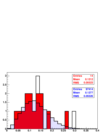
Figure 11: Observed (red, filled – upper box) and simulated (blue, hatched – lower box) redshift distribution. The two empty bins are SNe for which the host galaxy magnitude is fainter than cuts (5) or (6). A Kolmogorov-Smirnov test gives a 85 % probability of adequacy between the two distributions.

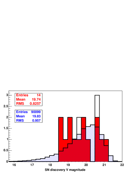
Figure 12: Observed (red, filled – upper box) and simulated (blue, hatched – lower box) discovery $V$ magnitude distribution. The two empty bins are SNe for which the host galaxy magnitude is fainter than cuts (5) or (6). A Kolmogorov-Smirnov test gives a 62 % probability of adequacy between the two distributions.

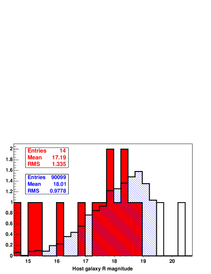
Figure 13: Observed (red, filled – upper box) and simulated (blue, hatched – lower box) host galaxy $R$ magnitude distribution. The two empty bins are SNe for which the host galaxy magnitude is fainter than cuts (5) or (6). A Kolmogorov-Smirnov test gives a 23 % probability of adequacy between the two distributions.

The distribution of the distance between the supernova and the host center is shown in Fig. 14. The Monte Carlo distribution was generated assuming that the supernova rate is proportional to the local surface brightness. The observed distribution is more concentrated toward the center than the surface brightness with the KS test giving a 3 % probability for compatibility. This suggests supernovae do not have the same distribution as the light though the limited statistics prevent any firm conclusion. At any rate, except far from galactic centers, our detection efficiency is nearly independent of the distance to the host center so the precise distribution of the distance has little effect on the global efficiency. All type of host galaxies are included in the simulated distribution. The observed distribution confirms that we are able to detect supernovae in the center of their host galaxies.

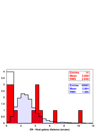
Figure 14: Observed (red, filled – upper box) and simulated (blue, hatched – lower box) distance to host distribution. The two empty bins are SNe for which the host galaxy magnitude is fainter than cuts (5) or (6). A Kolmogorov-Smirnov test gives a 3 % probability of adequacy between the two distributions. The simulated distribution assumes that the type Ia supernova rate is proportional to the galaxy surface brightness.

These checks being done, we are able to compute the rate, as the ratio of the number of detected supernovae to the integral value calculated as above. From the 1999 search we have 12 type Ia supernovae. But cut (5) on the galaxy host magnitude discards two events (SN 1999bl and SN 1999bn). In 2000, four type Ia supernovae were detected. Only 14 events remain after the cut. We can rewrite eq. (3) as

$$\mathcal{R}_{\text{SN}}=\frac{\mathcal{N}_{\text{tot}}}{\mathcal{I}_{\text{tot}}},$$ (15)

where $\mathcal{N}_{\text{tot}}$ is the total number of events surviving the cuts, and $\mathcal{I}_{\text{tot}}$ is the corresponding value of the integral. For the 1999 search, the integral is $\mathcal{I}^{99}=0.89\times 10^{14}\ h_{70}^{-2}\ \text{L}_{\odot}^{R}\ \text{yr}$, while it is $\mathcal{I}^{00}=0.50\times 10^{14}\ h_{70}^{-2}\ \text{L}_{\odot}^{R}\ \text{yr}$ for the 2000 search. The combined value of the integral for the two searches is the sum $\mathcal{I}_{\text{tot}}=\mathcal{I}^{99}+\mathcal{I}^{00}=1.39\times 10^{14}\ h_{70}^{-2}\ \text{L}_{\odot}^{R}\ \text{yr}$. Assuming the number of observed supernovae follows a Poisson law, with a confidence level of 68.3 %, one has $\mathcal{N}_{\text{tot}}=14^{+4.83}_{-3.70}$. This gives $\mathcal{R}_{Ia}^{R}=0.100^{+0.035}_{-0.027}\ h_{70}^{2}\ \text{SNu}_{R}$, where 1 SNu_R is 1 supernova/$10^{10}\ \text{L}_{\odot}^{R}$/century. The errors are only statistical at this point. The mean redshift for this value is given by the mean of the simulated redshift distribution (Fig. 11), that is $\langle z\rangle\ =0.128$. The calculated r.m.s. width of this redshift distribution is 0.056.

8.1 Systematic uncertainties

We have identified four possible sources of systematics: the calibration for both supernovae and galaxies, the cosmological model and the assumed distributions of supernova luminosities and light-curve shapes. For each of these parameters, various simulations have been performed to quantify the corresponding impact on the rate.

8.1.1 Calibration

We estimate the uncertainty on the zero point of eq. (12) to be of 0.07 mag (see Fig. 10). An increase (resp. decrease) in the zero point of 7 % decreases (resp. increases) the rate by 6 %.

Considering the galaxy calibration, eq. (13), we estimate an uncertainty on the zero point of about 0.1 mag (as combination of statistical error in the ensemble zeropoint error along with a possible systematic calibration error). An increase (resp. decrease) of the zero point by 10 % increases the rate by 7 % (resp. decreases the rate by 6 %). The net effect is lower than the 10 % due to luminosity alone, because the calibration for the redshift distribution acts in the opposite way.

8.1.2 Cosmology

The calculations and simulations have been done with the ($\Omega_{M_{\circ}},\ \Omega_{\Lambda_{\circ}}$) = (0.3, 0.7) cosmological model. We checked that using the ($\Omega_{M_{\circ}},\ \Omega_{\Lambda_{\circ}}$) = (1, 0) model lowers the rate by about 1 %. Only the probability density $p(z|m_{g})$, the galaxy luminosities and the supernovae magnitude (see eq. (LABEL:eqn:m1m2)), through the luminosity distance, depend on the cosmological model. But while the luminosity distance increases from (1, 0) model to (0.3, 0.7) model, on the contrary, the $p$ distribution is shifted toward the lower redshifts for a given apparent magnitude. The two effects cancel in this redshift range, hence the very small dependence of the cosmological parameters on the rate.

8.1.3 Supernova diversity

To take into account the fact that the distribution of supernovae luminosities and light-curve shapes is currently uncertain due to a lack of statistics, we parametrized the rate with the two main variables describing the type Ia variety distribution, the mean absolute magnitude at maximum $\langle M_{\text{V}_{\text{max}}}+5\log h_{70}\rangle$, and the light curve shape parameter $\langle\Delta m_{15}^{B}\rangle$ (Hamuy et al. 1996) for the 17 light curves we have used to derive the rate (see Fig. 7 and 8). Then we compute the following empirical relation:

$$\begin{split}&\left(\frac{\mathcal{R}_{\text{Ia}}}{0.100\ h_{70}^{2}\ \text{SNu}_{R}}\right)=\left(\frac{\langle\Delta m_{15}^{B}\rangle}{1.138}\right)^{0.65}\\ &\quad\times\left[1+0.78\cdot(\langle M_{\text{V}_{\text{max}}}+5\log h_{70}\rangle+18.55)\right],\end{split}$$ (16)

for deviations up to $\sim$ 20 % for $\langle M_{\text{V}_{\text{max}}}+5\log h_{70}\rangle$ and up to 10 % for $\langle\Delta m_{15}^{B}\rangle$. If the whole type Ia variety distribution is shifted, either in luminosity or in light curve shape parameter, as statistics increase with future experiments, our rate value will be able to be adjusted accordingly to eq. (16).

The uncertainty on the mean of the peak luminosity distribution (Fig. 7) of $\sim 0.96/\sqrt{17}=0.23$ mag translates into an uncertainty on the rate of $0.78\times 0.23=0.18$. The uncertainty on the mean value of $\Delta m_{15}^{B}$ (Fig. 8), of $0.257/\sqrt{17}=0.062$, translates into an uncertainty on the rate of 4 %. Then, the main source of uncertainty on the rate comes from the mean value of the peak luminosity distribution of supernovae.

If we remove the lowest luminosity supernova (SN 1996ai – see Fig. 7) from our reference sample, the rate is decreased by 16 %.

8.1.4 Supernovae in dim galaxies

Our search strategy requires an association to a host galaxy. This prevents detecting supernovae appearing in low brightness galaxies whose magnitude is beyond the detection threshold. For example, with such a cut, the type Ia SN 1999bw supernova, the host of which is a very low brightness dwarf galaxy (Strolger et al. 2002), would not have been detected by EROS (this supernova had a $B$ magnitude of 16.9 at maximum light, while its host has a $B$ magnitude of 24.2). Gal-Yam et al. (2003) also found two hostless type Ia supernovae in galaxy clusters. They argue that these events can be due to a putative intergalactic star population.

Since we assume that the number of supernovae is proportional to the host galaxy luminosity, the derived rate is independent of the galaxy luminosity cut (eq. (5) and (6)) (apart from statistical fluctuation). Then such an eventuality is included in our rate derivation as long as our working hypothesis is valid. Moreover we remark that these events are very rare, most probably representing a small fraction of events in the field.

Calibration:	SNe	$\pm 6\ \%$
	galaxies	${}_{-6\ \%}^{+7\ \%}$
SNe light curve distribution:	$\langle\Delta m_{15}^{B}\rangle$	$\pm 4\ \%$
	$\langle M_{V_{\text{max}}}\rangle$	$\pm 18\ \%$
Total (quadratic sum)		$\pm 21\ \%$

Table 2: Summary of identified systematic errors. The resulting total systematic uncertainty can be compared to the statistical uncertainty: ${}^{+39\ \%}_{-23\ \%}$.

8.2 The rate

Table 2 summarizes the error budget as discussed above. Taking it into account gives for the rate, the value:

$$\mathcal{R}_{\text{Ia}}^{R}=0.100^{+0.035+0.021}_{-0.027-0.021}\ h_{70}^{2}\ \text{SNu}_{R},$$ (17)

where the first quoted error is statistical and the second systematic. This number comes naturally in the $R$ band. However, the SN rate is traditionally expressed per luminosity unit in the $B$ band. We can convert this measurement into the $R$ band as:

$$\frac{\mathcal{R}_{\text{Ia}}^{B}}{\mathcal{R}_{\text{Ia}}^{R}}=\frac{L_{\text{gal}}^{R}}{L_{\odot}^{R}}\cdot\frac{L_{\odot}^{B}}{L_{\text{gal}}^{B}}=10^{-0.4\cdot[(B-R)_{\odot}-(B-R)_{\text{gal}}]}.$$ (18)

Using $(B-R)_{\odot}=1.06$ and $(B-R)_{\text{gal}}=1.3$ as the mean of the whole galaxy sample of Grogin & Geller (1999); we take $\pm 0.1$ mag as a possible systematic between our galaxy sample and theirs. Then, we have

$$\frac{L_{\text{gal}}^{R}}{L_{\odot}^{R}}\cdot\frac{L_{\odot}^{B}}{L_{\text{gal}}^{B}}=1.25\pm 0.11,$$ (19)

which gives:

$$\mathcal{R}_{\text{Ia}}^{B}=0.125^{+0.044+0.028}_{-0.034-0.028}\ h_{70}^{2}\ \text{SNu},$$ (20)

where the uncertainty which appears in the right hand side of eq. (19) has been added quadratically to the systematic error.

To obtain the rate per comoving volume unit, we multiply the value in eq. (20) by the mean galaxy luminosity density. The 2dF Galaxy Redshift Survey (Cross et al. 2001) provides a value at a mean redshift of 0.1, in the $B$ band and for a (1, 0) cosmological model, in agreement with the one obtained by the ESO Slice Project (Zucca et al. 1997). We translate the 2dF value to a (0.3, 0.7) model ($\left.j^{(0.3,\leavevmode\nobreak\ 0.7)}/j^{(1,\leavevmode\nobreak\ 0)}\right|_{z=0.1}=0.91$): $j_{B}\leavevmode\nobreak\ =\leavevmode\nobreak\ (1.59\pm 0.13)\times 10^{8}\ h_{70}\ \text{L}_{\odot}\ \text{Mpc}^{-3}$. The supernova rate (20) can then be expressed as:

$$\mathcal{R}_{\text{Ia}}=(1.99^{+0.70+0.47}_{-0.54-0.47})\times 10^{-5}\ h_{70}^{3}\ \text{yr}^{-1}\text{Mpc}^{-3}.$$ (21)

Here, the uncertainty on the luminosity density function has been added quadratically to the systematic error bar.

9 Discussion

9.1 Comparison with other measurements

Table 3 shows other published results for the type Ia supernova rate at various redshifts. Our measurement compares well with other measurements in the nearby universe (Cappellaro et al. 1999; Hardin et al. 2000; Madgwick et al. 2003). It is slightly lower but compatible within error bars. We note that our SN search strategy and our supernova sample are very different from those of Cappellaro et al. (1999) and Madgwick et al. (2003). The former used a sample of nearby supernovae discovered either by eye or on photographic plates which introduced large systematic errors in the rate. The latter used a new search technique based on galaxy spectra: supernovae are discovered in subtracting 116 000 galaxy spectra from the Sloan Digital Sky Survey by a eigenbasis of 20 “unpolluted” galaxy spectra. The method is very promising, especially in deriving the rate as a function of host galaxy properties.

On the other hand our rate is lower than the distant Pain et al. (2002) value, by over one standard deviation, either for the rate as a function of galaxy luminosity or as a function of comoving volume.

	$R_{\textrm{SN Ia}}$
$\langle z\rangle$	($h_{70}^{2}$ SNu)	($10^{-5}\ h_{70}^{3}\ \text{Mpc}^{-3}\ \text{yr}^{-1}$)	($\Omega_{M_{\circ}},\Omega_{\Lambda_{\circ}}$)	SNe nb	author
$\sim$ 0	$0.18\pm 0.05$	2.8$\pm$0.9		70	Cappellaro et al. (1999)a
0.098	0.196 $\pm$ 0.098	$3.12\pm 1.58$		19	Madgwick et al. (2003)a
0.13	$\mathbf{0.125^{+0.044+0.028}_{-0.034-0.028}}$	$\mathbf{1.99^{+0.70+0.47}_{-0.54-0.47}}$	(0.3, 0.7)	14	this work
0.14	$0.22^{+0.17+0.06}_{-0.10-0.03}$	$3.43^{+2.7+1.1}_{-1.6-0.6}$	(0.3, 0.7)	4	Hardin et al. (2000)a,b
$0.25^{+0.12}_{-0.07}$	$0.20^{+0.82}_{-0.19}$		(0.3, 0.7)	1	Gal-Yam et al. (2002)c
0.38	$0.40^{+0.26+0.18}_{-0.18-0.12}$		(1.0, 0.0)	3	Pain et al. (1996)
0.46		$4.8\pm 1.7$	(0.3, 0.7)	8	Tonry et al. (2003)
0.55	$0.28^{+0.05+0.05}_{-0.04-0.04}$	$5.25^{+0.96+1.10}_{-0.86-1.06}$	(0.3, 0.7)	38	Pain et al. (2002)
0.55	$0.46^{+0.08+0.07}_{-0.07-0.0.7}$	$11.1^{+2.0+1.1}_{-1.8-1.1}$	(1.0, 0.0)	38	Pain et al. (2002)
$0.90^{+0.37}_{-0.07}$	$0.40^{+1.21}_{-0.38}$		(0.3, 0.7)	5	Gal-Yam et al. (2002)c

Table 3: Comparison with other published restframe type Ia supernova explosion rate measurements. These rates are given together with the mean redshift of the observed SNe and the cosmological model assumed (especially for distant values). The fifth column gives the number of supernovae from which the rate is computed. Notes: $a$) the value per comoving volume unit is derived from the SNu value using the 2dF luminosity density (the error on the luminosity density is added quadratically to the systematic uncertainty if distinct); $b$) Hardin et al. (2000) computed the rate using a ($\Omega_{M_{\circ}},\Omega_{\Lambda_{\circ}}$) = (0.3, 0.0) cosmological model. Nevertheless no important difference from the (0.3, 0.7) model is expected (less than 10%); $c$) Gal-Yam et al. (2002) have measured the rate in galaxy clusters, with could be different from the rate in the field; they do not give a value per unit of comoving volume.

9.2 Evolution?

Our result combined with the SCP measurement at higher redshift (Pain et al. 2002) suggests models with an evolution of the rate, either in SNu or per unit of comoving volume, between $z=0.13$ and $z=0.55$. We can parametrize such evolution as a power-law: $\mathcal{R}_{\text{Ia}}(z)=\mathcal{R}_{\text{Ia}}(0)\cdot(1+z)^{\alpha}$ where $\alpha$ is a restframe evolution index. Using the present result and the Pain et al. (2002) value per unit of comoving volume, we obtain $\alpha_{v}=3.1^{+1.6}_{-1.4}$. The same parameter computed for the rate expressed in SNu is $\alpha_{l}=2.6^{+1.5}_{-1.3}$. The difference, $\alpha_{v}-\alpha_{l}=0.5\pm 0.1$, simply reflects the different luminosity densities adopted by us and Pain et al. (2002), equivalent to an evolving luminosity density with $\alpha_{j_{B}}^{\text{SNe}}=0.5\pm 0.1$. In fact, the luminosity density most likely evolves a bit faster. Combining the data of Lilly et al. (1996) with that of Cross et al. (2001) and imposing a (0.3, 0.7) cosmological model, the evolution of the luminosity density corresponds to $\alpha_{j_{B}}^{\text{Lilly}}=0.73\pm 0.51$. If Pain et al. (2002) had adopted a luminosity density more in line with this value of $\alpha_{j_{B}}$ then we would have deduced $\alpha_{l}=2.4^{+1.7}_{-1.5}$ by combining our data with that of Pain et al. (2002). This number is still significantly greater than zero.

The value of $\alpha_{v}=3.1^{+1.6}_{-1.4}$ derived by combining our data with that of Pain et al. (2002) is consistent with the value $\alpha_{v}=0.8\pm 1.6$ derived using only the Pain et al. (2002) data.

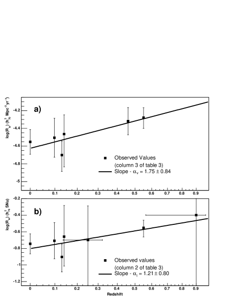
Figure 15: Derivation of the evolution index $\alpha$ using all available SNIa rate measurements (see Table 3), within the (0.3, 0.7) cosmological model.

Nevertheless, fitting all available rate measurements either in SNu or per comoving volume unit, provides a lower evolution index (see Fig. 15): $\alpha_{v}=1.75\pm 0.84$ and $\alpha_{l}=1.21\pm 0.80$.

Models such as those by Madau et al. (1998) or by Sadat et al. (1998) can fit the observations (Fig. 16). In the Madau et al. (1998) models, the evolution depends not only on the time delay between the white dwarf formation and the supernova explosion, but also on the galaxy formation scenario, especially at high redshift. In these models the supernova rate follows roughly a $(1+z)^{\alpha_{v}}$ evolution with $\alpha_{v}\gtrsim 1.8$ ($\tau=0.3$), $\alpha_{v}\sim 2.4$ ($\tau=3$) up to $\alpha_{v}\sim 2.8$ ($\tau=1$). The Sadat et al. (1998) models depend on the choice of star formation rate evolution model and on dust extinction. They predict $\alpha_{v}\sim 1.4$ for “M1” model and $\alpha_{v}\sim 1.8$ for the “M2” model.

Too few data points exist up to now in order to constrain accurately many parameters from the models, such as the galaxy formation scenario (Madau et al. 1998) (only good quality data at redshift $\gtrsim 1.5$ could eventually distinguish between the two favored galaxy formation scenarios), the progenitor model (Ruiz-Lapuente & Canal 1998), environmental effects like the metallicity (Kobayashi et al. 2000) or the cosmology (Dahlén & Fransson 1999).

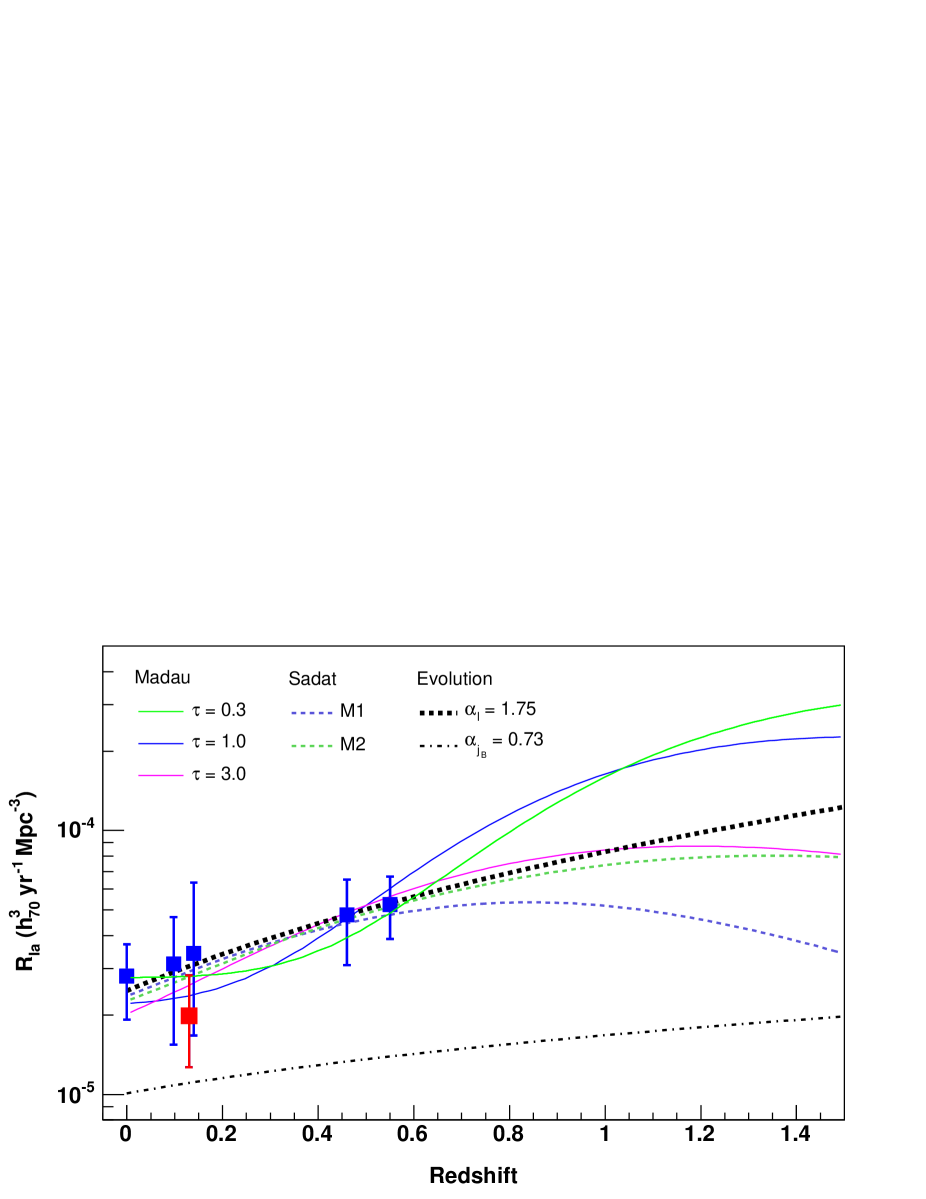
Figure 16: Explosion rate evolution per unit of time and comoving volume. The set of curves labeled “Madau” stands for the models by Madau et al. (1998), computed within the hierarchical clustering galaxy formation scenario; $\tau$ is the time interval between the white dwarf formation and the supernova explosion (in Gyr). The curves labeled “Sadat” stand for the Sadat et al. (1998) models, using two different star formation rate evolution models (M1 and M2, the latter accounts for a possible dust extinction correction). From left to right are the measured values by Cappellaro et al. (1999), Madgwick et al. (2003), this work, Hardin et al. (2000), Tonry et al. (2003) and Pain et al. (2002). We plot also the redshift evolution, $(1+z)^{1.75}$, corresponding to the best fit using the six measured values. The effect of the evolution of the galaxy luminosity density ($\alpha_{j_{B}}$) is shown as well since it is included in the rate per comoving volume unit evolution. All data points and model curves have been computed with the (0.3, 0.7) cosmological model, and $h_{70}=1$. The normalisation of models is set by adjusting them to the data.

9.3 Conclusion

We have measured the type Ia supernova explosion rate at a redshift of 0.13. Combined with other measurements at different redshifts, it suggests a slight evolution of the rate with the redshift. Nevertheless, the scatter and the still large error bars of the current measurements do not allow us to make definite conclusions about it.

Future supernova searches will shed more light on the rate evolution. Among them, two dedicated supernova searches, are well suited to improve and measure the evolution of the explosion rate. The Nearby Supernova Factory (Aldering et al. 2002) is a nearby ($z\lesssim 0.1$) supernova search using two dedicated telescopes, one for the search and one for the follow-up of discovered events using an integral field spectrometer. It will be very helpful to measure the local supernova rate using a very homogeneous set of a few hundred events, and it will also help reducing the uncertainties on the supernova light curve distribution. Another supernova search in progress uses the wide field Megacam camera on the CFHT. Supernovae are discovered in a rolling search mode up to $z\lesssim 0.9$; it will be possible to use them for measuring the evolution of the explosion rate for type Ia supernovae at a 15 % level of statistical uncertainty (per bin of 0.1 in redshift). Concerning other supernova searches well suited to compute the explosion rate, we can quote the Sloan Digital Sky Survey performing a spectroscopic detection of nearby supernovae, as already mentioned (Madgwick et al. 2003); the Lick Observatory and Tenagra Observatory Supernova Searches detecting nearby event using automatic telescopes; at intermediate redshifts ($z\sim 0.4$), the ESO Supernova Search is designed to search for supernovae in order to derive the rate; in the distant Universe, the Great Observatories Origins Deep Survey Treasury program is searching for very distant type Ia supernovae using the Hubble Space Telescope.