Simulations of Turbulent Thermonuclear Burning in
Type Ia Supernovae

1 Summary

Type Ia supernovae, i.e. stellar explosions which do not have hydrogen in their spectra, but intermediate-mass elements such as silicon, calcium, cobalt, and iron, have recently received considerable attention because it appears that they can be used as “standard candles” to measure cosmic distances out to billions of light years away from us. Observations of type Ia supernovae seem to indicate that we are living in a universe that started to accelerate its expansion when it was about half its present age. These conclusions rest primarily on phenomenological models which, however, lack proper theoretical understanding, mainly because the explosion process, initiated by thermonuclear fusion of carbon and oxygen into heavier elements, is difficult to simulate even on supercomputers.

Here, we investigate a new way of modeling turbulent thermonuclear deflagration fronts in white dwarfs undergoing a type Ia supernova explosion. Our approach is based on a level set method which treats the front as a mathematical discontinuity and allows for full coupling between the front geometry and the flow field. New results of the method applied to the problem of type Ia supernovae are obtained. It is shown that in 2-D with high spatial resolution and a physically motivated subgrid scale model for the nuclear flames numerically “converged” results can be obtained, but for most initial conditions the stars do not explode. In contrast, simulations in 3-D, do give the desired explosions and many of their properties, such as the explosion energies, lightcurves and nucleosynthesis products, are in very good agreement with observed type Ia supernovae.

2 Introduction

Numerical simulations of any kind of turbulent combustion have always been a challenge, and thermonuclear supernova explosions are no exception to that rule. This is mainly because of the large range of length scales involved. In type Ia supernovae (SNe Ia), in particular, the length scales of relevant physical processes range from 10^-3cm for the Kolmogorov-scale to several 10⁷cm for typical convective motions. In the currently favored scenario the explosion starts as a deflagration near the center of the star. Rayleigh-Taylor unstable blobs of hot burnt material are thought to rise and to lead to shear-induced turbulence at their interface with the unburnt gas. This turbulence increases the effective surface area of the flamelets and, thereby, the rate of fuel consumption; the hope is that finally a fast deflagration might result, in agreement with phenomenological models of type Ia explosions.

Despite considerable progress in the field of modeling turbulent combustion for astrophysical flows the correct numerical representation of the thermonuclear deflagration front has always been a weakness of the simulations. Methods used until recently were based on the reactive-diffusive flame model, which artificially stretches the burning region over several grid zones to ensure an isotropic flame propagation speed. However, the soft transition from fuel to ashes stabilizes the front against hydrodynamical instabilities on small length scales, which in turn results in an underestimation of the flame surface area and – consequently – of the total energy generation rate. Moreover, because nuclear fusion rates depend on temperature nearly exponentially, one cannot use the zone-averaged values of the temperature obtained this way to calculate the reaction kinetics.

The front tracking method used in this project cures most of these weaknesses. It is based on the so-called level set technique which was originally introduced by Osher & Sethian (1988). They used the zero level set of a $n$-dimensional scalar function to represent $(n-1)$-dimensional front geometries. Equations for the time evolution of such a level set which is passively advected by a flow field are given in Sussman et al. (1994). The method has been extended to allow the tracking of fronts propagating normal to themselves, e.g. deflagrations and detonations (Smiljanovski et al., 1997). In contrast to the artificial broadening of the flame in the reaction-diffusion-approach, this algorithm is able to treat the front as an exact hydrodynamical discontinuity.

3 The level set method

The central aspect of our front tracking method is the association of the front geometry (a time-dependent set of points $\Gamma$) with an isoline of a so-called level set function $G$:

$$\Gamma:=\{\vec{r}\ |\ G(\vec{r})=0\}.$$ (1)

Since $G$ is not completely determined by this equation, we can additionally postulate that $G$ be negative in the unburnt and positive in the burnt regions, and that $G$ be a “smooth” function, which is convenient from a numerical point of view. This smoothness can be achieved, for example, by the additional constraint that $|\vec{\nabla}G|=1$ in the whole computational domain, with the exception of possible extrema and kinks of $G$. The ensemble of these conditions produces a $G$ which is a signed distance function, i.e. the absolute value of $G$ at any point equals the minimal front distance. The normal vector to the front is defined to point towards the unburnt material.

The task is now to find an equation for the temporal evolution of $G$ such that the zero level set of $G$ behaves exactly as the flame. Such an expression can be obtained by the consideration that the total velocity of the front consists of two independent contributions: it is advected by the fluid motions at a speed $\vec{v}$ and it propagates normal to itself with a burning speed $s$.

Since for deflagration waves a velocity jump usually occurs between the pre-front and post-front states, we must explicitly specify which state $\vec{v}$ and $s$ refer to; traditionally, the values for the unburnt state are chosen. Therefore, one obtains for the total front motion

$$\vec{D}_{f}=\vec{v}_{u}+s_{u}\vec{n}.$$ (2)

The total temporal derivative of $G$ at a point $P$ attached to the front must vanish, since $G$ is, by definition, always 0 at the front:

$$\frac{\text{d}G_{P}}{\text{d}t}=\frac{\partial G}{\partial t}+\vec{\nabla}G\cdot\dot{\vec{x}}_{P}=\frac{\partial G}{\partial t}+\vec{D}_{f}\cdot\vec{\nabla}G=0$$ (3)

This leads to the desired differential equation describing the time evolution of $G$:

$$\frac{\partial G}{\partial t}=-\vec{D}_{f}\cdot\vec{\nabla}G.$$ (4)

This equation, however, cannot be applied on the whole computational domain, mainly because using this equation everywhere will in most cases destroy $G$’s distance function property. Therefore additional measures must be taken in the regions away from the front to ensure a “well-behaved” $|\vec{\nabla}G|$ (Reinecke et al., 1999).

The situation is further complicated by the fact that the quantities $\vec{v}_{u}$ and $s_{u}$ which are needed to determine $\vec{D}_{f}$ are not readily available in the cells cut by the front. In a finite volume context, these cells contain a mixture of pre- and post-front states instead. Nevertheless one can assume that the conserved quantities (mass, momentum and total energy) of the mixed state satisfy the following conditions:

$$\overline{\rho} =\alpha\rho_{u} +(1-\alpha)\rho_{b}$$ (5)

$$\overline{\rho\vec{v}} =\alpha\rho_{u}\vec{v}_{u} +(1-\alpha)\rho_{b}\vec{v}_{b}$$ (6)

$$\overline{\rho e} =\alpha\rho_{u}e_{u} +(1-\alpha)\rho_{b}e_{b}$$ (7)

Here $\alpha$ denotes the volume fraction of the cell occupied by the unburnt state. In order to reconstruct the states before and behind the flame, a nonlinear system consisting of the equations above, the Rankine-Hugoniot jump conditions and a burning rate law must be solved.

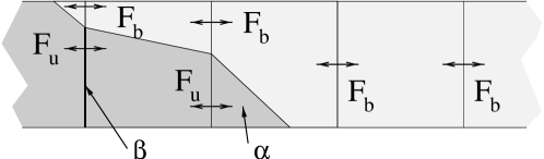
Figure 1: Illustration of the basic principles of the level set method according to Smiljanovski et al. (1997): The piecewise linear front cuts the mixed cells into burnt and unburnt parts. $\alpha$ is the unburnt volume fraction of a cell, $\beta$ is the unburnt area fraction of a cell interface. The fluxes $\vec{F}_{u}$ and $\vec{F}_{b}$ are calculated from the reconstructed states.

Having obtained the reconstructed pre- and post-front states in the mixed cells, it is not only possible to determine $\vec{D}_{f}$, but also to separately calculate the fluxes of burnt and unburnt material over the cell interfaces. Consequently, the total flux over an interface can be expressed as a linear combination of burnt and unburnt fluxes weighted by the unburnt interface area fraction $\beta$ (see Fig. 1):

$$\vec{\bar{F}}=\beta\vec{F}_{u}+(1-\beta)\vec{F}_{b}.$$ (8)

4 Implementation

For our calculations, the front tracking algorithm was implemented as an additional module for the hydrodynamics code PROMETHEUS (Fryxell et al., 1989). Here we describe a simple implementation of most of the ideas discussed in the previous section which we will call “passive implementation”. It assumes that the $G$-function is advected by the fluid motions and by burning and is only used to determine the source terms for the reactive Euler equations. It must be noted that there exists no real discontinuity between fuel and ashes in this case; the transition is smeared out over about three grid cells by the hydro-dynamical scheme, and the level set only indicates where the thin flame front should be. However, the numerical flame is still considerably thinner than in the reaction-diffusion approach.

A complete implementation contains in-cell-reconstruction and flux-splitting as proposed by Smiljanovski et al. (1997) and outlined above. Therefore it describes exactly the coupling between the flame and the hydrodynamic flow. This generalized version of the code has been applied to hydrogen combustion in air by Reinecke et al. (1999) and, very recently, also to thermonuclear fusion by Röpke et al. (2003).

4.1 $G$-Transport

Since the front motion consists of two distinct contributions, it is appropriate to use an operator splitting approach for the time evolution of $G$. The advection term due to the fluid velocity $\vec{v}_{F}$ reads in conservation form

$$\int_{V}\frac{\partial(\rho G)}{\partial t}d^{3}r+\oint_{\partial V}-\vec{v}_{F}\rho Gd\vec{f}=0$$ (9)

(Mulder et al., 1992). This equation is identical to the advection equation of a passive scalar, like the concentration of an inert chemical species. Consequently, this contribution to the front propagation can be calculated by PROMETHEUS directly. The additional flame propagation due to burning is calculated at the end of each time step and a re-initialization of $G$ is done in order to keep it a signed distance function (see Reinecke et al. 1999).

4.2 Source terms

After the update of the level set function in each time step, the change of chemical composition and total energy due to burning is calculated in the cells cut by the front. In order to obtain these values, the volume fraction $\alpha$ occupied by the unburnt material is determined in those cells by the following approach: from the value $G_{ij}$ and the two steepest gradients of $G$ towards the front in $x$- and $y$-direction a first-order approximation $\tilde{G}$ of the level set function is calculated; then the area fraction of cell $ij$ where $\tilde{G}<0$ can be found easily. Based on these results, the new concentrations of fuel, ashes and energy are obtained:

$$X^{\prime}_{\text{Ashes}} =\text{max}(1-\alpha,X_{\text{Ashes}})$$ (10)

$$X^{\prime}_{\text{Fuel}} =1-X^{\prime}_{\text{Ashes}}$$ (11)

$$e^{\prime}_{\text{tot}} =e_{\text{tot}}+q(X^{\prime}_{\text{Ashes}}-X_{\text{Ashes}})$$ (12)

In principle this means that all fuel found behind the front is converted to ashes and the appropriate amount of energy is released. The maximum operator in eq. (10) ensures that no “reverse burning” (i.e. conversion from ashes to fuel) takes place in the cases where the average ash concentration is higher than the burnt volume fraction; such a situation can occur in a few rare cases because of unavoidable discretization errors of the numerical scheme.

5 Turbulent nuclear burning

The system of equations described so-far can be solved provided the normal velocity of the burning front is known everywhere and at all times. In our computations it is determined according to a flame-brush model of Niemeyer & Hillebrandt (1995a), which we will briefly outline for convenience.

As was mentioned before, nuclear burning in degenerate dense matter is believed to propagate on microscopic scales as a conductive flame, wrinkled and stretched by local turbulence, but with essentially the laminar velocity. Due to the very high Reynolds numbers macroscopic flows are highly turbulent and they interact with the flame, in principle down to the Kolmogorov scale. This means that all kinds of hydrodynamic instabilities feed energy into a turbulent cascade, including the buoyancy-driven Rayleigh-Taylor instability and the shear-driven Kelvin-Helmholtz instability. Consequently, the picture that emerges is more that of a “flame brush” spread over the entire turbulent regime rather than a wrinkled flame surface. For such a flame brush, the relevant minimum length scale is the so-called Gibson scale, defined as the lower bound for the curvature radius of flame wrinkles caused by turbulent stress. Thus, if the thermal diffusion scale is much smaller than the Gibson scale (which is the case for the physical conditions of interest here) small segments of the flame surface are unaffected by large scale turbulence and behave as unperturbed laminar flames (“flamelets”). On the other hand side, since the Gibson scale is, at high densities, several orders of magnitude smaller than the integral scale set by the Rayleigh-Taylor eddies and many orders of magnitude larger than the thermal diffusion scale, both transport and burning times are determined by the eddy turnover times, and the effective velocity of the burning front is independent of the laminar burning velocity.

A numerical realization of this general concept is presented in Niemeyer & Hillebrandt (1995a). The basic assumption was that wherever one finds turbulence this turbulence is fully developed and homogeneous, i.e. the turbulent velocity fluctuations on a length scale $l$ are given by the Kolmogorov law $v(l)=v(L)(l/L)^{1/3}$, where $L$ is the integral scale, assumed to be equal to the Rayleigh-Taylor scale. Following the ideas outlined above, one can also assume that the thickness of the turbulent flame brush on the scale $l$ is of the order of $l$ itself. With these two assumptions and the definition of the Gibson scale one finds for $l_{\mathrm{gibs}}\lessapprox l\lessapprox L\simeq\lambda_{\mathrm{RT}}$

$$v(l)\simeq s_{\mathrm{t}}(l)\simeq s_{\mathrm{t}}(l_{\mathrm{gibs}})\biggl{(}\frac{l}{l_{\mathrm{gibs}}}\biggr{)}^{1/3}$$ (13)

and $d_{t}(l)\simeq l$, where $v(l_{\mathrm{gibs}})=s_{\mathrm{lam}}$ defines $l_{\mathrm{gibs}}$, $s_{\mathrm{lam}}$ is the laminar burning speed and $s_{\mathrm{t}}(l)$ is the turbulent flame velocity on the scale $l$.

In a second step this model of turbulent combustion is coupled to our finite volume hydro scheme. Since in every finite volume scheme scales smaller than the grid size cannot be resolved, we express $l_{\mathrm{gibs}}$ in terms of the grid size $\Delta$, the (unresolved) turbulent kinetic energy per unit mass, $k_{\mathrm{sgs}}$, and the laminar burning velocity:

$$l_{\mathrm{gibs}}=\Delta\biggl{(}\frac{u_{l}^{2}}{2k_{\mathrm{sgs}}}\biggr{)}^{3/2}.$$ (14)

Here $k_{\mathrm{sgs}}$ is determined from a subgrid scale model (Clement, 1993; Niemeyer & Hillebrandt, 1995a) and, finally, the effective turbulent velocity of the flame brush on scale $\Delta$ is given by

$$s_{\mathrm{t}}(\Delta)=\operatorname{max}(s_{\mathrm{lam}},v(\Delta),v_{\mathrm{RT}}),$$ (15)

with $v(\Delta)=\sqrt{2k_{\mathrm{sgs}}}$ and $v_{\mathrm{RT}}\propto\sqrt{g\Delta}$, where $g$ is the local gravitational acceleration.

6 Application to the supernova problem

Different series of simulations were performed to check the numerical reliability of the employed models and to compare two- and three-dimensional explosions.

Figure 2: Time evolution of the total energy for identical initial conditions at different resolutions. While model c3_2d_128 is clearly under-resolved, the other simulations agree very well, at least in the early and intermediate stages.

6.1 Resolution study

A crucial test for the validity of the models for the unresolved scales (in this case the flame and subgrid models) is to check the dependence of integral quantities, like the total energy release of the explosion, on the numerical grid resolution. Ideally, there should be no such dependence, indicating that all effects on unresolved scales are accurately modeled.

Figure 2 shows the energy evolution of a centrally ignited white dwarf. The only difference between the simulations is the central grid resolution, which ranges from $2\cdot 10^{6}$cm (model c3_2d_128) down to $2.5\cdot 10^{5}$cm (model c3_2d_1024). Model c3_2d_128 is obviously under-resolved, but the results of the other calculations are in good agreement, with exception of the last stages, where the flame enters strongly non-uniform regions of the grid.

So far, this kind of parameter study could only be performed in two dimensions, because of the prohibitive cost of very highly resolved 3D simulations. Nevertheless the results suggest that a resolution of $\approx 10^{6}$cm should yield acceptable accuracy also in three dimensions.

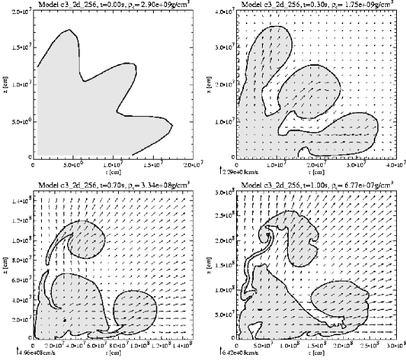
Figure 3: Burning front geometry evolution of model c3_2d_256.

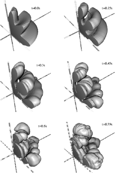
Figure 4: Burning front geometry evolution of model c3_3d_256. One ring on the axes corresponds to $10^{7}$cm.

Figure 5: Comparison of the energy evolution for identical initial conditions in two and three dimensions.

6.2 Comparison of 2D and 3D simulations

In order to investigate the fundamental differences between two- and three-dimensional simulations, a 2D and a 3D model with identical initial conditions and resolution was calculated. Figures 3 and 4 show snapshots of the flame geometry at various explosion stages; the energy evolution of both models is compared in figure 5.

It is evident that both simulations evolve nearly identically during the first few tenths of a second, as was expected. This is a strong hint that no errors were introduced into the code during the enhancement of the numerical models to three dimensions. At later times, however, the 3D calculation develops instabilities in the azimuthal direction, which could not form in 2D because of the assumed axial symmetry. As a consequence the total burning surface and the energy generation rate is increased, resulting in a higher overall energy release.

6.3 The effect of different initial conditions

In our approach, the initial white dwarf model (composition, central density, and velocity structure), as well as assumptions about the location, size and shape of the flame surface as it first forms fully determine the simulation results. At present, we have not changed the properties of the white dwarf but we concentrate on variations of the latter. In this context, the simultaneous runaway at several different spots in the central region of the progenitor star is of particular interest, a plausible ignition scenario suggested by Garcia-Senz & Woosley (1995).

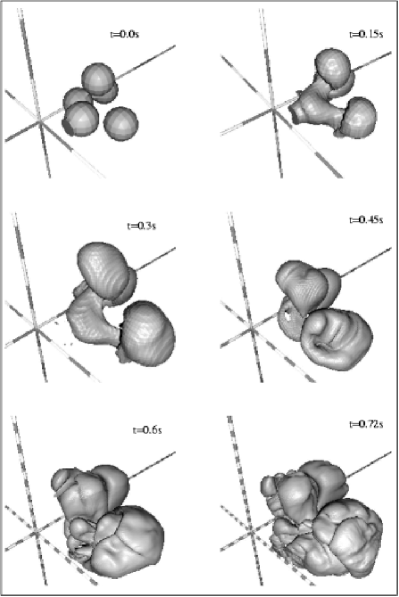
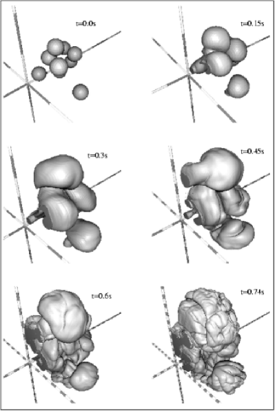
Figure 6: Left panel: Snapshots of the flame front for a scenario with 5 ignition spots in 3D. The fast merging between the leading and trailing bubbles and the rising of the entire burning region is clearly visible. One ring on the coordinate axes corresponds to $10^{7}$cm. Right panel: The same as before, but for a high resolution model with 9 ignition spots.

Figure 7: Energy evolution of these three-dimensional explosion models (dashed and dashed-dotted). For comparison we also show the centrally ignited (“three fingers”) model of Reinecke et al. (2002) (solid line) discussed earlier.

One simulation was carried out on a grid of 256³ cells with a central resolution of 10⁶ cm and contained five bubbles with a radius of 3$\cdot$10⁶ cm, which were distributed randomly in the simulated octant within 1.6$\cdot$10⁷ cm of the star’s center. In an attempt to reduce the initially burned mass as much as possible without sacrificing too much flame surface, a very highly resolved second model was constructed. It contains nine randomly distributed, non-overlapping bubbles with a radius of 2$\cdot$10⁶ cm within 1.6$\cdot$10⁷ cm of the white dwarf’s center. To properly represent these very small bubbles, the cell size was reduced to $\Delta=$5$\cdot$10⁵ cm, so that a total grid size of $512^{3}$ cells was required.

During the first 0.5 seconds, the three models are nearly indistinguishable as far as the total energy is concerned (see Fig. 7), which at first glance appears somewhat surprising, given the quite different initial conditions. A closer look at the energy generation rate actually reveals noticeable differences in the intensity of thermonuclear burning for the simulations, but since the total flame surface is initially very small, these differences have no visible impact on the integrated curve in the early stages.

However, after about 0.5 seconds, when fast energy generation sets in, the nine-bubble model burns more vigorously due to its larger surface and therefore reaches a higher final energy level. Fig. 7 also shows that the centrally ignited model (c3_3d_256) is almost identical to the off-center model b5_3d_256 with regard to the explosion energetics. But, obviously, the scatter in the final energies due to different initial conditions appears to be small. Moreover, all models explode with an explosion energy in the range of what is observed.

7 Predictions for observable quantities

In this Section we present a few preliminary results for various quantities which could, in principle, be observed and which therefore can serve as tests for the models.

7.1 Lightcurves

The most direct test of explosion models is provided by observed lightcurves and spectra. According to “Arnett’s Law” lightcurves measure mostly the amount and spatial distribution of radioactive ⁵⁶Ni in type Ia supernovae, and spectra measure the chemical composition in real and velocity space.

Sorokina & Blinnikov (2003) have used the results of one of our centrally ignited 3D-model, averaged over spherical shells, to compute colour lightcurves in the UBVI-bands. Their code assumes LTE radiation transport and loses reliability at later times (about 4 weeks after maximum) when the supernova enters the nebular phase. Also, this assumption and the fact that the opacity is not well determined at longer wavelength make I-lightcurves less accurate. Keeping this in mind, the lightcurves shown in Fig. 8 look very promising. The main reason for the good agreement between the model and SN 1994D is the presence of radioactive Ni in outer layers of the supernova model at high velocities which is not be predicted by spherical models.

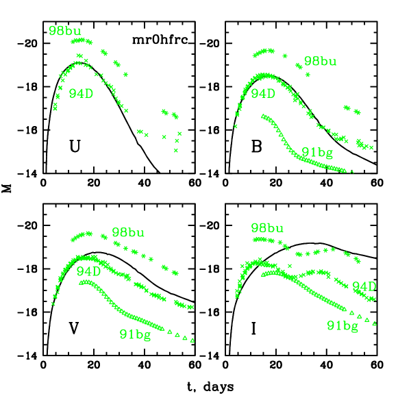
Figure 8: UBVI-colour lightcurves predicted by a centrally ignited 3D model (solid lines) in comparison with obseved data for a bright (98bu), a “normal” (94D), and a subluminous (91bg) supernova.

7.2 Elemental and isotopic abundances

A summary of the abundances obtained for all 3D models is given in Table 1. Here “Mg” (as in Fig. 8) stands for intermediate-mass nuclei, and “Ni” for the iron-group. In addition, the total energy liberated by nuclear burning is given. Since the binding energy of the white dwarf was about 5$\cdot$10⁵⁰ erg, all models do explode. Typically one expects that around 80% of iron-group nuclei are originally present as ⁵⁶Ni bringing our results well into the range of observed Ni-masses. This success of the models was obtained without introducing any non-physical parameters, but just on the basis of a physical and numerical model of subsonic turbulent combustion. We also stress that our models give clear evidence that the often postulated deflagration-detonation transition is not needed to produce sufficiently powerful explosions.

model name $m_{\text{Mg}}$ [$M_{\odot}$] $m_{\text{Ni}}$ [$M_{\odot}$] $E_{\text{nuc}}$ [$10^{50}$ ergA] c3_3d_256 0.177 0.526 9.76 b5_3d_256 0.180 0.506 9.47 b9_3d_512 0.190 0.616 11.260

Table 1: Overview over element production and energy release of all discussed supernova simulations

Finally, we have “post-processed” one of our models in order to see whether or not also reasonable isotopic abundances are obtained. The results, shown in Fig. 9, are preliminary and should be considered with care. However, it is obvious that, with a few exceptions, also isotopic abundances are within the expected range and do not differ too much from those computed by means of phenomenological models, i.e. “W7”. Exceptions include the high abundance of (unburned) C and O, and the overproduction of ^48,50Ti, ⁵⁴Fe, and ⁵⁸Ni.

Figure 9: Isotopic abundances obtained for off-center ignited 3D model.

8 Supplementary studies

In order to validate our approach to model the effects on unresolved scales, two studies were carried out. One tests several subgrid scale (SGS) models under the physical conditions encountered in SN Ia explosions and the other concerns the flame stability on small scales, where the turbulent cascade does not dominate the flame evolution.

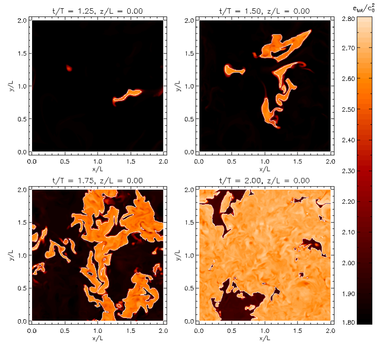
Figure 10: Evolution of turbulent thermonuclear burning in a cubic domain subject to periodic boundary conditions. The panels show 2D contour sections of the normalized specific total energy, $e_{\mathrm{tot}}/c_{0}^{2}$. The mean mass density is $\rho_{0}\approx 2.903\cdot 10^{8}\,\mathrm{g\,cm^{-3}}$ and the initial sound speed $c_{0}\approx 6.595\cdot 10^{8}\,\mathrm{cm\,s^{-1}}$. Turbulence is produced artificially by a stochastic solenoidal force field. The bright regions of high specific energy contain burned material. The flame front is indicated by the thin white lines corresponding to the zero level set.

Figure 11: Comparison of the evolution of SGS turbulence and thermonuclear burning for LES with three different variants of the SGS turbulence energy model. In one simulation, Clement’s law of the wall was used to calculate the closure parameters, the second LES was computed with the constant parameters and for the third simulation, a semi-localized model was applied. In the top panels, the ratio of the mean SGS turbulence velocity to the RMS velocity and the laminar burning speed, respectively, is shown as function of normalized time $t/T$. In the middle row of panels, the first three statistical moments of the mass-weighted SGS turbulence velocity and, in the bottom panels, the time evolution of fuel, burning products and the mean energy generation rate are plotted.

8.1 Large eddy simulations of turbulent deflagration

Subgrid scale models were tested in large eddy simulations (LES) of thermonuclear burning in a turbulent flow. In these simulations, turbulence is driven by an artificial stochastic force field and the computational domain is cubic with periodic boundary conditions. The term large eddy simulation indicates that not all dynamic scales are numerically resolved. Compared to simulations of supernova explosions, there are two additional differences: Firstly, the periodic boundary conditions enforce a constant average mass density. Hence, there is no explosion in this setting. The burning process proceeds in the form of a percolation process as gradually all fuel is consumed and the system approaches a state in which degenerate C+O matter is replaced by ⁵⁶Ni and $\alpha$ particles in statistical nuclear equilibrium. Secondly, gravity is not included. Since the integral length scale is of the order $10^{5}\,\mathrm{cm}$, this is a sensible approximation. In consequence, we focus on the interaction of the deflagration with purely hydrodynamical turbulence for which the similarity theory of Kolmogorov applies. Whether SGS models which do not account for effects induced by gravity are applicable to thermonuclear supernova explosions is still controversial. However, there are simple scaling arguments in favor of this conjecture. The single most important result emerging from our studies is that the evolution of the burning process is significantly affected by the SGS model in use. This underlines the importance of choosing a faithful SGS model and certainly bears consequences on the simulation of deflagration in SNe Ia.

Our approach of determining the turbulent flame speed as outlined in Section 5 is based upon a dynamical equation for the SGS turbulence energy $k_{\mathrm{sgs}}=\frac{1}{2}q_{\mathrm{sgs}}^{2}$ which can be casted into the following equation for the turbulence velocity $q_{\mathrm{sgs}}$:

$$\frac{\mathrm{D}}{\mathrm{D}t}q_{\mathrm{sgs}}-\frac{1}{\rho}\nabla\cdot\left(\rho\ell_{\kappa}q_{\mathrm{sgs}}\nabla q_{\mathrm{sgs}}\right)-\ell_{\kappa}|\nabla q_{\mathrm{sgs}}|^{2}=\ell_{\nu}|S^{\ast}|^{2}-\left(\frac{1}{3}+\frac{C_{\lambda}}{2}\right)q_{\mathrm{sgs}}d-\frac{q_{\mathrm{sgs}}^{2}}{\ell_{\epsilon}}$$ (16)

The operator $\frac{\mathrm{D}}{\mathrm{D}t}$ is the Lagrangian time derivative $\frac{\partial}{\partial t}+\vec{v}\cdot\nabla$. In this equation, several heuristic approximations, so-called closures, are incorporated. Associated with these closures are the length scales $\ell_{\nu}=C_{\nu}\Delta_{\mathrm{eff}}/\sqrt{2}$, $\ell_{\epsilon}=2\sqrt{2}\Delta_{\mathrm{eff}}/C_{\epsilon}$ and $\ell_{\kappa}=C_{\kappa}\Delta_{\mathrm{eff}}/\sqrt{2}$. $C_{\lambda}$ accounts for pressure effects in a compressible fluid. The closure parameters $C_{\nu}$, $C_{\epsilon}$, $C_{\kappa}$ and $C_{\lambda}$ are a priori unknown. In the case of stationary isotropic turbulence in an incompressible fluid, values can be derived from analytic theories of turbulence. Particular examples are $C_{\nu}\approx 0.054$, $C_{\epsilon}\approx 1.0$ and $C_{\kappa}\approx 0.1$ (cf. Sagaut (2001), Section 4.3) and $C_{\lambda}\approx-0.2$ (Fureby et al., 1997). $\Delta_{\mathrm{eff}}$ is the effective length scale of the finite-volume scheme, in this case, the piece-wise parabolic method. Usually, this scale is set equal to the size $\Delta$ of the grid cells. However, from the energy spectra of direct numerical simulations (DNS) of forced isotropic turbulence, we concluded that is more appropriate to set $\Delta_{\mathrm{eff}}=\beta\Delta$, where $\beta$ is in the range $1.6\ldots 1.8$ depending on the Mach number. The factor $\beta$ accounts for the smoothing effect of the numerical scheme on top of the discretization.

We have also determined statistical values of the closure parameters from DNS data. For subsonic flows, $C_{\nu}=0.06$, $C_{\epsilon}=0.48$ and $C_{\kappa}=0.36$ appear to be representative values. The outcome of a LES of turbulent deflagration in a cube of $216^{3}$ cells with these parameters is illustrated in Figure 10. Burning is ignited in eight small spherical zones at the beginning of the simulation and the fluid is set into motion by stochastic forcing. Turbulence is produced on a time scale $T=L/V$, where $L=2.16\cdot 10^{5}\,\mathrm{cm}$ is the integral length scale and $V=100s_{\mathrm{lam}}\approx 9.78\cdot 10^{7}\,\mathrm{cm\,s^{-1}}$ is the characteristic velocity of the flow. One can think of $L$ being the typical size of the largest vortices generated by the stochastic force field and $T$ is the associated autocorrelation time or, figuratively, the turn-over time. Initially, the burning zones are expanding very slowly as the flame propagation speed mostly equals the laminar speed. After roughly one turn-over time has elapsed, SGS turbulence becomes increasingly space filling and enhances the flame propagation speed. At the same time, the folding and stretching of the flame front by the resolved flow greatly increases the surface and, thus, the rate of fuel consumption. These two effects appreciably accelerate the burning process as one can see from the evolution of the energy shown in Figure 10. At time $t\gtrsim 2T$, most of the material has already been burnt.

Constant closure parameters are a sensible choice for fully developed isotropic turbulence. However, significant deviations are expected for transient, intermittent or anisotropic flows. The deflagration in the cube is certainly transient and, naturally, the physical conditions in the vicinity of the flame front are anisotropic. In the case of a supernova explosion, these qualities are even more pronounced. For this reason, a more sophisticated method of determining the closure parameters is called for. Clement (1993) found for stellar structure modeling ad hoc rules to adjust the parameters $C_{\nu}$ and $C_{\epsilon}$ in order to account for compressibility in stratified media. Since steep density gradients affect turbulence more or less like a wall, we shall refer to the rules proposed by Clement as “law of the wall”. This method has been applied to SGS modeling in the simulations of thermonuclear supernovae as well. In comparison to the SGS turbulence energy model with constant parameters, Clement’s law of the wall produces markedly different results as one can seen from the LES statistics plotted in Figure 11. The mean of $q_{\mathrm{sgs}}$ increases initially very rapidly and then settles at an almost constant level. Correspondingly, the average rate of energy release per unit volume due to thermonuclear burning, $\langle B\rangle$, increases more gradually as opposed to steep rise and high peak found for the SGS model with constant parameters.

An entirely different method utilizes the filtering approach introduced by Germano (1992). Smoothing the resolved velocity field with a filter of characteristic length larger than $\Delta_{\mathrm{eff}}$ and invoking self-similarity assumptions, equations can be derived which yield closure parameters varying in space and time corresponding to the local structure and evolution of the flow. (Piomelli, 1993; Liu et al., 1994; Ghosal et al., 1995; Meneveau & Katz, 2000). This so-called dynamical procedure works particularly well for the production parameter $C_{\nu}$. In the case of dissipation and diffusion, however, the method appears to be inadequate because of deficiencies in the respective closures. Therefore, we adopted a semi-localized approach. Results from a LES using this method, are shown in the panels on the very right of Figure 11. The differences compared to the LES with constant parameters are not striking but Clement’s method is clearly dismissed. The prediction of the latter that SGS turbulence is produced right at the beginning in advance of small-scale structure developing in the resolved flow is physically unreasonable. Apart from that, once turbulence has developed in a particular spatial region, it becomes increasingly isotropic on decreasing length scales even in more complex flows. Thus, the remarkable similarity of the evolution of the burning process in the LES with constant and dynamical parameters, respectively. However, the choice of appropriated values for the closure parameters is notoriously difficult, particularly, when it comes to the supernova explosion scenario in which turbulence is generated due to buoyancy effects originating from the density contrast between burnt and unburnt material. In conclusion, the semi-localized model is likely to be the preferable SGS model for the application to SNe Ia simulations after all.

8.2 Investigation of the cellular burning regime

Figure 12: Flame propagation into quiescent fuel at $\rho_{u}=5\times 10^{7}\,\mathrm{g}\,\mathrm{cm}^{-3}$, resolution: $200\times 200$ cells, snapshots taken at (a) 0, (b) 7.5, (c) 15, and (d) 30 growth times $\tau_{\mathrm{LD}}$ of a perturbation with $\lambda=3.2\times 10^{4}\,\mathrm{cm}$. Color-coded is the vorticity of the flow field. (The figure is also included in the color plates of this volume.)

Below the Gibson scale, flame propagation is not dominated by the turbulent cascade, since here the flame burns faster through turbulent eddies than these can deform it. On those scales flame evolution is determined by the (hydrodynamical) Landau-Darrieus (LD) instability (Landau, 1944) and its counteracting nonlinear stabilization (Zel’dovich, 1966). In case of terrestrial flames this stabilization leads to a cellular steady-state pattern of the flame front giving rise to the cellular burning regime. After Niemeyer & Hillebrandt (1995b) have shown by means of hydrodynamical simulation that the LD instability acts under conditions of SNe Ia, we could confirm that also the cellular stabilization of the flame front holds for thermonuclear flames in white dwarfs. This was achieved in a series of 2D simulations. In order to reproduce hydrodynamical effects like the LD instability it turned out to be essential to apply the complete implementation described in Sect. 3 (see Röpke et al. 2003). The stability of this cellular flame shape was tested for various fuel densities and for interaction of the flame with vortical flows. Two examples are given in the following.

Figure 12 shows the propagation of an initially perturbed flame into quiescent fuel. The initial perturbations grow and in the nonlinear regime the flame exhibits a cellular structure. For the given setup, however, the cellular pattern of the same wavelength as the initial perturbation is not a stable solution. The snapshots at later times (Fig. 12b,c) illustrate the “merging” of cells until the steady-state structure of a single domain-filling cusp has formed. In case of higher numerical resolution, this fundamental flame structure may be superposed by a short-wavelength cellular pattern, which is advected toward the cusp and does not lead to a break-up of the domain-filling cell. This evolution is well in agreement with theoretical predictions. Simulations with different fuel densities $\rho_{u}$ led to similar results. In the range of $\rho_{u}=1\times 10^{7}\,\mathrm{g}\,\mathrm{cm}^{-3}\ldots 1\times 10^{9}\,\mathrm{g}\,\mathrm{cm}^{-3}$ no significant flame destabilization could be observed.

Flame interaction with a vortical fuel field is shown in Fig. 13. This is motivated by relic turbulent motions from the eddy cascade around the Gibson scale and from pre-ignition convective motions in the white dwarf. A parameter study with different fuel densities and various strengths of the velocity fluctuations in the fuel flow led to the result that a vortical flow of sufficient strength can break up the cellular pattern of the flame. In this case, however, no drastic self-turbulization of the flame but rather a smooth adaptation of the flame structure to the imprinted flow was observed.

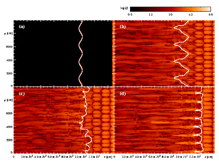
Figure 13: Flame propagation into vortical fuel at $\rho_{u}=5\times 10^{7}\,\mathrm{g}\,\mathrm{cm}^{-3}$; velocity fluctuations at the right boundary: $v^{\prime}/u_{\mathrm{lam}}=2.5$; resolution: $300\times 200$ cells; snapshots taken at (a) $0\,\mathrm{s}$, (b) $8.0\times 10^{-3}\,\mathrm{s}$, (c) $1.6\times 10^{-2}\,\mathrm{s}$, and (d) $4.8\times 10^{-2}\,\mathrm{s}$. Color-coded is the vorticity of the flow field. (The figure is also included in the color plates of this volume.)

These results corroborate the assumption of large scale models, that the generation of turbulence is dominated by large-scale effects. In the cellular burning regime, the flame surface is enlarged compared to a planar configuration. This leads to an additional acceleration of the flame. As a result of our study we suggest an increased lower cut-off of the flame velocity (cf. eq. (15)) instead of $u_{\mathrm{lam}}$ depending on background turbulence.

9 Conclusion

In this project, we have provided a new method to model the physics of thermonuclear combustion in degenerate dense matter of white dwarfs stars consisting of carbon and oxygen. Because not all relevant length-scales of this problem can be numerically resolved a numerical model to describe deflagration fronts with a reaction zone much thinner then the cells of the computational grid was presented. This new approach was applied to the simulate thermonuclear supernova explosions of $M_{\rm Chan}$ white dwarfs in 2 and 3 dimensions.

An implicit assumption of our numerical model is that on the resolved scales the flows are turbulent allowing us to describe the physics on the unresolved scales by a subgrid scale model, in the spirit of large-eddy simulations. The results presented here indicate that for supernova simulations this assumption is satisfied if we compute 3D models and use at least a 256³ grid. The reason is simply that more structure on small length scales in better resolved models increases the rate of fuel consumption locally, but the turbulent velocity fluctuations are then smaller on the grid scale, compensating for this gain.

All models we have computed (differing only in the ignition conditions and the grid resolution) explode. The explosion energy and the Ni-masses are only moderately dependent on the way the nuclear flame is ignited making the explosions robust. However, since ignition is a stochastic process, the differences we find may even explain some of the spread in observed SN Ia’s.

Based on our models we can predict lightcurves, spectra, and abundances, and the first preliminary results look promising. The lightcurves seem to be in very good agreement with observations, and also the nuclear abundances of elements and their isotopes are found to be in the expected range. Of course, the next step is to compute a grid of models, with varying white dwarf properties, and to compare them with the increasing data base of well-observed type Ia supernovae. The hope is that this will give us a tool to understand their physics and, thus, get confidence in their use for cosmology.

10 Acknowledgements

The numerical computations presented here were in part carried out on the Hitachi SR-8000 at the Leibniz-Rechenzentrum München as a part of the project H007Z. We thank the staff of the HLRB at the LRZ for their continous help.

This work was also supported in part by the Deutsche Forschungsgemeinschaft under Grant Hi 534/3-3.

References

- Clement (1993) Clement, M. J.: 1993, ApJ 406, 651
- Fryxell et al. (1989) Fryxell, B. A., Müller, E., Arnett, W. D.: 1989, MPA Preprint 449
- Fureby et al. (1997) Fureby, C., Tabor, G., Weller, H. G., Gosman, A. D.: 1997, Phys. of Fluids 9, 3578
- Garcia-Senz & Woosley (1995) Garcia-Senz, D., Woosley, S. E.: 1995, ApJ 454, 895
- Germano (1992) Germano, M.: 1992, J. Fluid Mech. 238, 325
- Ghosal et al. (1995) Ghosal, S., Lund, T. S., Moin, P., Akselvoll, K.: 1995, J. Fluid Mech. 286, 229
- Landau (1944) Landau, L. D.: 1944, Acta Physicochim. URSS 19, 77
- Liu et al. (1994) Liu, S., Meneveau, C., Katz, J.: 1994, J. Fluid Mech. 275, 83
- Meneveau & Katz (2000) Meneveau, C., Katz, J.: 2000, Ann. Rev. Fluid Mech. 32, 1
- Mulder et al. (1992) Mulder, W., Osher, S., Sethian, J. A.: 1992, J. Comput. Phys. 100, 209
- Niemeyer & Hillebrandt (1995a) Niemeyer, J. C., Hillebrandt, W.: 1995a, ApJ 452, 769
- Niemeyer & Hillebrandt (1995b) Niemeyer, J. C., Hillebrandt, W.: 1995b, ApJ 452, 779
- Osher & Sethian (1988) Osher, S., Sethian, J. A.: 1988, J. Comput. Phys. 79, 12
- Piomelli (1993) Piomelli, U.: 1993, Phys. of Fluids 5, 1484
- Reinecke et al. (2002) Reinecke, M. A., Hillebrandt, W., Niemeyer, J. C.: 2002, A&A 386, 936
- Reinecke et al. (1999) Reinecke, M. A., Hillebrandt, W., Niemeyer, J. C., Klein, R., Gröbl, A.: 1999, A&A 347, 724
- Röpke et al. (2003) Röpke, F. K., Niemeyer, J. C., Hillebrandt, W.: 2003, ApJ 588, 952
- Sagaut (2001) Sagaut, P.: 2001, Large eddy simulation for incompressible flows, Springer
- Smiljanovski et al. (1997) Smiljanovski, V., Moser, V., Klein, R.: 1997, Comb. Theory and Modeling 1, 183