Constraining Born-Infeld models of dark energy with CMB anisotropies

Abstract

We study the CMB constraints on two Dark Energy models described by scalar fields with different Lagrangians, namely a Klein-Gordon and a Born-Infeld field. The speed of sound of field fluctuations are different in these two theories, and therefore the predictions for CMB and structure formation are different. Employing the WMAP data on CMB, we make a likelihood analysis on a grid of theoretical models. We constrain the parameters of the models and compute the probability distribution functions for the equation of state. We show that the effect of the different sound speeds affects the low multipoles of CMB anisotropies, but is at most marginal for the class of models studied here.

Introduction

Several observations now indicate WMAP ; SN that the universe has been accelerating its expansion rate for the last 5 – 10 Gy. Standard candidates for the “dark energy” (DE) which is responsible for this recent burst of expansion are a cosmological constant and a scalar field RP ; accellera ; kessence ; japan ; AF03 which, for reasons unknown yet, started to dominate over the other types of matter just at our cosmological era. Unfortunately, DE seems to pose an even more formidable problem than that of dark matter to observational cosmology: whereas we still hope that the particles that make up dark matter will eventually be detected, and that incremental knowledge about the distribution of large-scale sctructure and galactic dynamics will eventually nail down the basic properties of dark matter and its relation to baryonic matter, no such hopes apply for DE, at least for now. Nevertheless, we must not shy away from trying to test models of DE, under penalty of theory running amok.

One of the best opportunities to test DE is by looking at the anisotropies in the temperature and polarization of the cosmic microwave background radiation (CMB), which have been measured with exquisite accuracy by WMAP WMAP — and will be measured with even grander precision by the PLANCK mission PLANCK .

There are basically two ways through which DE can affect the CMB. The first is through its impact on the expansion rate, which is determined by the equation of state of the DE component. The second is directly through the perturbations: DE, if it is not a plain cosmological constant, possesses small inhomogeneities which interact gravitationally with the inhomogeneities in baryons, dark matter and relativistic matter. The physical properties of DE perturbations constitute additional ingredients which can impact the CMB anisotropies and LSS.

Here we are interested in the role of the sound speed of DE perturbations. Whereas for the background evolution it is only necessary to specify the DE budget at the present time $\Omega_{X\,0}$, and its pressure/density ratio $w_{X}(t)=p_{X}(t)/\rho_{X}(t)$, in order to classify the perturbations sector we need to specify the pressure perturbations as well erickson :

$$\delta p_{X}=c_{X}^{2}\delta\rho_{X}+3H(1+w_{X})\frac{\theta_{X}\rho_{X}}{k^{2}}\left(c_{X}^{2}-\frac{\dot{p}_{X}}{\dot{\rho}_{X}}\right)\,,$$ (1)

where $\rho_{X}$, $\delta\rho_{X}$, $c_{X}^{2}$ and $\theta_{X}$ are respectively the DE density, density perturbation, sound speed and velocity potential. The case for a perfect fluid DE model in which $\delta p_{X}=c_{X}^{2}\delta\rho_{X}$ has been analyzed in CF and compared with the WMAP data in AFBC . In this paper we focus on the scalar field case in which the pressure perturbation is not simply related to the density perturbation.

The standard quintessence scenario (a canonical scalar field described by a Klein-Gordon Lagrangian) is a minimal modification to $\Lambda$CDM, and in that particular case $c_{X}^{2}=1$. All the information contained in the scalar potential $V(\varphi)$ is encoded in $w_{X}$ in that case.

The possibility of having $c_{X}^{2}\neq 1$ in the context of scalar field theories by considering a Lagrangian with a non-standard kinetic term is not new. If such non-canonical scalar field plays the role of an inflaton, the predictions for scalar and tensor perturbations are different with respect to the usual (canonical) scenario kinflation . In the context of DE, K-essence kessence was proposed (see also japan ), even if it has the unpleasant feature of having fluctuations which can travel with speeds faster than that of light. The imprints of K-essence on CMB anisotropies have already been studied elsewhere erickson ; kessence_pheno , but not yet in a statistic way. Here we focus on a different scalar field theory and we perform a statistical study of the predictions .

To be concrete we study a Klein-Gordon (KG henceforth) Lagrangian density:

$${\cal{L}}_{KG}=-\sqrt{-g}\,\left[\frac{1}{2}\partial^{\mu}\varphi\partial_{\mu}\varphi+V(\varphi)\right]\;,$$ (2)

and compare it to a Born-Infeld borninfeld (BI henceforth) Lagrangian

$${\cal{L}}_{BI}=-V(\phi)\sqrt{1+\frac{\partial^{\mu}\phi\partial_{\mu}\phi}{M^{4}}}$$ (3)

(where we have assumed a signature $(-+++)$ for the metric and we have introduced the mass scale $M$). This Lagrangian can be thought as a field theory generalization of the Lagrangian of a relativistic particle padma . For $\partial^{\mu}\phi\partial_{\mu}\phi/M^{4}<<1$, by taking the first term of a Taylor expansion of Eq. (3), we get a Lagrangian which is equivalent to the KG one by redefining the field (except for problems with the invertibility of this redefinition). Only by taking the full Lagrangian (3), the two theories are different. The BI was recently revisited in connection with string theory, since it seems to represent a low-energy effective theory of D-branes and open strings Sen ; gg . In the case of constant potential, the model reduces to a type of hydrodynamical matter known as the Chaplygin Gas Chap — whose predictions were studied in CF ; AFBC . While for the KG Lagrangian the sound speed of fluctuations is $1$ independently of the potential, in the BI case $c_{X}^{2}=-w_{X}\geq 0$ always, regardless of the potential.

For both theories we will assume an inverse power-law potential:

$$V(f)=\frac{m^{4+p}}{f^{p}}\;,$$ (4)

where $p>0$ and $f$ stands for $\varphi$ or $\phi$ in the canonical or non-canonical cases, respectively. Positive powers of the field ($p<0$) yield models which, if not finely tuned, do not lead to acceleration. In the following we split the fields as $f=f_{0}(t)+\delta f(t,{\bf x})$, as usually done in cosmology.

Equation of state versus sound speed

In the canonical case, the scalar field model with potential (4) is known as the Ratra-Peebles model of dark energy RP . In the BI case it was shown in AF03 that this model can lead to an accelerating regime when $p\leq 2$. With the potential given by Eq. (4), both theories behave very similarly at the level of the background. This is so because both scalar fields possess fluid-like attractor solutions when the background energy density is dominated by a perfect fluid such as dust ($w_{F}=0$) or radiation ($w_{F}=1/3$). For the Ratra-Peebles model the equation of state of the attractor during a fluid-dominated period is ZWS :

$$w_{\varphi}=\frac{\frac{1}{2}\dot{\varphi}_{0}^{2}-V(\varphi_{0})}{\frac{1}{2}\dot{\varphi}_{0}^{2}+V(\varphi_{0})}\simeq\frac{p\,w_{F}-2}{p+2}\;,$$ (5)

where $\varphi_{0}(t)$ is the homogeneous value of the scalar field. For the BI model the equation of state during a fluid-dominated period is AF03 :

$$w_{\phi}=-1+\frac{\dot{\phi}_{0}^{2}}{M^{4}}\simeq-1+p\frac{1+w_{F}}{2}\;.$$ (6)

In particular, for $p\ll 1$, $w_{\varphi}\simeq w_{\phi}$, while tracking is more and more accurate for $p>>1$ in the KG case and for $p\simeq 2$ in the BI case.

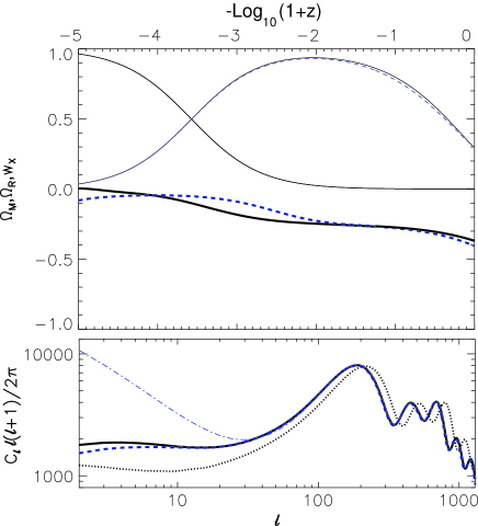
Figure 1: Upper panel: background quantities for two similar Born-Infeld (BI, dashed lines) and Klein-Gordon (KG, solid lines) dark energy models as a function of redshift. The upper curves denote $\Omega_{r}$ and $\Omega_{m}$, and the lower, nearly superimposed curves denote the equations of state for the two models. The cosmological parameters are $\Omega_{b}=0.04$, $\Omega_{m}=0.26$, $h=0.72$, and either $p=3/2$ (BI) or $p=6$ (KG.) Lower panel: temperature angular power spectra for KG model (solid line), BI model (dashed line) and a fiducial $\Lambda$CDM (dotted line), all normalized at the location of their first doppler peak. Only for comparison we also show the (wrong) power spectrum of the BI model obtained without considering the scalar field perturbations (dot-dashed line).

The main difference between them lies in the behaviour of their perturbations. The canonical scalar field perturbations $\delta\varphi(x,t)$ obey the equation of motion:

$$\delta\ddot{\varphi}-\frac{\nabla^{2}}{a^{2}}\delta\varphi+3H\delta\dot{\varphi}+V_{,\varphi\varphi}\delta\varphi=-\frac{1}{2}\dot{h}\dot{\varphi}_{0}\;,$$ (7)

where $a$ is the scale factor and $h$ is the synchronous gauge metric perturbation. The BI scalar perturbation, on the other hand, obeys the equation:

$$\frac{\delta\ddot{\phi}}{1-\dot{\phi}_{0}^{2}/M^{4}} - \frac{\nabla^{2}}{a^{2}}\delta\phi+3H\delta\dot{\phi}+\frac{2\dot{\phi}_{0}\ddot{\phi}_{0}}{(1-\dot{\phi}_{0}^{2}/M^{4})^{2}}\delta\dot{\phi}$$ (8)

$$+ M^{4}(\log V)_{,\phi\phi}\delta\phi=-\frac{1}{2}\dot{h}\dot{\phi}_{0}\,.$$

Eqs. of motion (7) and (8) determine how perturbations behave: while the canonical scalar field perturbations have a speed of sound $c_{\varphi}^{2}=1$, in the BI case the speed of sound is $c_{\phi}^{2}=-w_{\phi}=1-\dot{\phi}_{0}^{2}/M^{4}$. Since $c_{X}^{2}$ determines how fast fluctuations dissipate, a lower sound speed increases the phase space of modes which are Jeans unstable beandore [to make contact with Eq. (1), $\theta_{X}=k^{2}\delta f/\dot{f}$, where $\delta f$ is the field perturbation.] Hence, the spectra of anisotropies predicted by the two models are slightly different because of the different Jeans scales in the DE sector – see Fig. 1.

A key feature of these models is that not only their backgrounds are well described by a simple attractor: their perturbations are funnelled to an attractor as well AF01 . This means that the issue of initial conditions for the background field and the perturbations is partially solved . If this was not true, initial conditions would constitute additional free parameters in the models.

CMB phenomenology and likelihood analysis

In order to compute the CMB anisotropies we employed a modified version of the code CMBFAST v. 4.1 CMBFAST , adding scalar fields to the system of equations.

We take the following vector of free parameters:

$$\vec{\alpha}=\{H,\Omega_{m},\Omega_{b},n_{s},m,p;A\}\;,$$ (9)

where $H$ denotes the present value of the Hubble constant in Km s^-1 Mpc^-1, $\Omega_{m}$ is the amount of dark matter, $\Omega_{b}$ the amount of baryons, $n_{s}$ is the scalar spectral index, $m$ is the scalar field mass scale in the potential (4) and $p$ is the power of the scalar potential. As always, there is a free parameter (A) related to the (unobservable) overall normalization of the CMB spectrum. Since we consider only flat models, the density in the dark energy component, $\Omega_{X}$, is fixed once the other cosmological parameters are determined. We have ommitted the BI scale $M$ from the space of parameters since it can be absorbed by a redefinition of $m$.

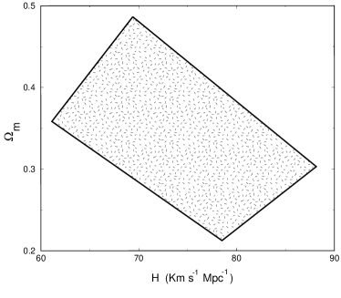
Figure 2: Region of $[H,\Omega_{m}]$ probed by our simulations.

We have evaluated the likelihood function $\mathcal{L}(C_{l}|\vec{\alpha})$ for a grid of roughly 370,000 models using the code described in verde . In order to get the posterior probability distribution function (p.d.f) for a given parameter, we must marginalize the likelihood function over the remaining ones. Since $\mathcal{L}(C_{l}|\vec{\alpha})$ is not a p.d.f in the usual sense, we use Bayes’ Theorem:

$$P(\alpha_{i})\propto\int\mathcal{L}(C_{l}|\vec{\alpha})\prod_{j\neq i}\mathcal{P}(\alpha_{j})d\alpha_{j}\;,$$ (10)

where $\mathcal{P}(\alpha_{j})$ is the prior p.d.f for $\alpha_{j}$.

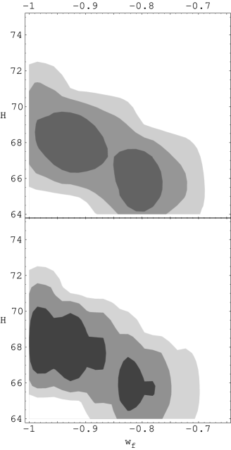
Figure 3: Joint posteriori p.d.f. for $H$ and $\omega_{f}$ from WMAP data, for Ratra-Peebles (upper panel) and Born-Infeld (lower panel) models. The shaded areas correspond to 1, 2 and 3$\sigma$ levels.

For the parameters in (9) we set an equally spaced grid with the following (flat) priors: 64 $\leq H\leq$ 80 , 0.036 $\leq\Omega_{b}\leq$ 0.069, 0.95 $\leq n_{s}\leq$ 1.09. In the matter era ($\omega_{F}=0$), the power $p$ of the potential can be substituted by $\omega_{f}$ because of Eqs. (5)-(6), so we chose a grid that was equally spaced in $\omega_{f}$ rather than $p$, with $-0.6\leq\omega_{f}\leq-1$. Regarding $\Omega_{m}$ and $H$, it was numerically more suitable to use a certain combination of the two parameters which effectively explored a region of parameter space whose shape is shown in Fig. 2.

We can study the parameters $H$ and $\omega_{f}$ (or, equivalently, $p$) jointly by marginalizing against (i.e., integrating out) all other parameters according to (10), thus obtaining the posteriori marginalized p.d.f. $P_{m}(H,\omega_{f})$. This joint p.d.f for $H$ and $\omega_{f}$ is presented in Fig. 3 for the models under scrutiny. The contours correspond to 1, 2 and $3\sigma$ levels. For the Ratra-Peebles (KG) case, the joint p.d.f for $H$ and $\omega_{f}$ agrees with CD .

We are mainly interested in $\omega_{f}$, so we marginalize against $H$ as well to obtain the posteriori p.d.f. for the equation of state of dark energy. The p.d.f’s, shown in Fig. 4, have been smoothed through a Bezier spline so that the effects of having an imperfect grid are not overestimated.

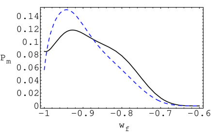
Figure 4: Probability distribution function as a function of the equation of state for both models: KG (solid line) and BI (dashed line.)

The limits on the equation of state of the dark energy component are, for the KG model:

$$\omega_{\varphi}>-0.84\,(1\sigma),\,-0.74\,(2\sigma),\,-0.68\,(3\sigma)\,,$$

where 1$\sigma$, 2$\sigma$ and 3$\sigma$ correspond to 68.3% C.L., 95.4% and 99.7% C.L., respectively. For the BI model the limits on its equation of state are:

$$\omega_{\phi}>-0.87(1\sigma),\,-0.76\,(2\sigma),\,-0.69\,(3\sigma)\,.$$ (11)

Conclusions

We have tested two scalar field models of dark energy against the WMAP data on CMB anisotropies. For simplicity we have taken the same potential for both Lagrangians. Our aim was to compare models which had nearly identical backgrounds, but whose perturbative sectors behave differently. We did this by comparing two scalar field models, a Klein-Gordon (the usual quintessence) and a Born-Infeld scalar, both of which have very similar attractor solutions during radiation- and matter-domination.

From a fundamental perspective, we have shown that a BI scalar field can easily play the role of DE. As for being a CDM candidate CDM the non-linear stage must still be carefully analyzed nonlinear . We stress that a very interesting feature of BI theories is that the BI scalar can act as dust and drive the universe into acceleration, where the trigger to the accelerated phase is the transition of the background from radiation-dominated to dust-dominated at $z_{eq}\sim 10^{4}$ AF03 .

For the Ratra-Peebles model (a canonical scalar field model) we find an allowed range of parameters $p<0.38$ at 1$\sigma$, corresponding to an equation of state during the attractor regime in the matter-dominated period of $-1\leq w_{\varphi}\leq-0.84$. The Born-Infeld model, on the other hand, is more tightly constrained: we find $p<0.27$ at 1$\sigma$, corresponding to an equation of state of the attractor regime of $-1\leq w_{\phi}\leq-0.87$. For the Born-Infeld model, this also implies a limit for the sound speed of dark energy $c_{\phi}^{2}>0.87$ at the $1\sigma$ level.

The effect of the perturbations was not dramatic in the BI case, since we have $c_{X}^{2}=-w_{X}$ (compared to $c_{X}^{2}=1$ for quintessence). However, in the cases studied here, the speed of sound affects interestingly the low-$\ell$ multipoles. In order to have a DE model which fits observations well, one has to consider $w_{X}\lesssim-0.5$ and therefore the sound speed for BI fluctuations is not sufficiently different from quintessence. Because of cosmic variance and high error bars, low $\ell$’s have a diminished influence on the Likelihood, which means that the region where the different perturbative behaviors show up more conspicuously are not well represented in the Likelihood analysis. Nevertheless, changing the speed of sound of dark energy by a factor of order 10% can have an impact (from the point of view of the Likelihoods) of the same order of magnitude as changing the other cosmological parameters by a few percent, which is the precision target of future experiments such as PLANCK PLANCK .

This reinforces the notion kessence_pheno that only dark energy models which possess a highly unusual perturbative behavior, such as certain models of k-essence kessence , models with $c_{X}^{2}\sim 0$ (and unrelated to $w_{X}$) or dark energy perfect fluids CF ; AFBC (where the pressure perturbation in Eq. (1) depends only on the density perturbation) can have a large impact on the CMB.

We would like to thank V. Mukhanov and I. Waga for useful conversations. F. F. would like to thank the Instituto de Física, Universidade de São Paulo, for its warm hospitality when this work was initiated. R. A. would like to thank the CNR/IASF and INFN - Bologna as well, for its hospitality. This work was also supported by FAPESP, CNPq and CAPES.

References

- (1) C. Bennett et al., Astrophys. J. Suppl. 148: 1 (2003); D.N. Spergel et al., idem 148: 175 (2003).
- (2) A. Riess et al, Astron. J. 116 (1998) 1009; P. Garnavich et al, Astrophys. J. (1998) 509 74; S. Perlmutter et al, Astrophys. J. 517 (1998) 565; J. Tonry et al., Astrophys. J. 594 (2003) 1, astro-ph/0305008.
- (3) B. Ratra and P. J. E. Peebles, Phys. Rev. D 37, 3406 (1988); C. Wetterich, Nucl. Phys. B 302, 645 (1988).
- (4) J. Frieman, C. Hill, A. Stebbins and I. Waga, Phys. Rev. Lett. 75, 2077 (1995); R. R. Caldwell, R. Dave and P. J. Steinhardt, Phys. Rev. Lett. 75, 2077 (1995); I. Zlatev, L.-M. Wang and P. J. Steinhardt, Phys. Rev. Lett. 75, 2077 (1995).
- (5) C. Armendariz-Picon, V. F. Mukhanov and P. J. Steinhardt, Phys. Rev. Lett. 85, 4438 (2000); Phys. Rev. D 63, 103510 (2001).
- (6) T. Chiba, T. Okabe and M. Yamaguchi, Phys. Rev. D 62, 023511 (2000).
- (7) L. R. Abramo and F. Finelli, Phys. Lett. B 575: 165 (2003).
- (8) http://astro.estec.esa.nl/SA-general/Projects/Planck/
- (9) J. K. Erickson et al., Phys. Rev. Lett. 88, 121301 (2002).
- (10) D. Carturan and F. Finelli, Phys. Rev. D 68, 103501 (2003).
- (11) L. Amendola, F. Finelli, C. Burigana and D. Carturan, JCAP 0307, 005 (2003).
- (12) J. Garriga and V. F. Mukhanov, Phys. Lett. B 458, 219 (1999); see also D. Steer and F. Vernizzi, hep-th/0310139.
- (13) S. DeDeo, R. R. Caldwell, P. Steinhardt, Phys. Rev. D 67, 103509 (2003).
- (14) R. Bean and O. Dore, Phys. Rev. D 69, 083503 (2004).
- (15) M. Born and L. Infeld, Proc. Roy. Soc. London A 144, 425 (1934).
- (16) T. Padmanabhan, Phys. Rev. D 66: 021301 (2002); J. Bagla, H. Jassal and T. Padmanabhan Phys. Rev. D67: 063504 (2003); M. Sami, P. Chingangbam and T. Qureshi, Phys. Rev. D66: 043530 (2002).
- (17) A. Sen, JHEP 0204: 048 (2002); ibid. 0207: 065 (2002); A. Sen, Mod. Phys. Lett. A17: 1797-1804 (2002).
- (18) G. W. Gibbons, Phys. Lett. B 537, 1 (2002).
- (19) R. Jackiw, arXiv physics/0010042; A. Kamenshchik, U. Moschella and V. Pasquier, Phys. Lett. B 511: 265 (2001); N. Bilic, G. Tupper and R. Viollier, Phys. Lett. B535: 17 (2002); M. C. Bento, O. Bertolami and A. A. Sen, Phys. Rev. D66: 043507 (2002).
- (20) P. J. Steinhardt, Li-Min Wang and Ivaylo Zlatev, Phys. Rev. D59: 123504 (1999)
- (21) L. R. Abramo and F. Finelli, Phys. Rev. D64: 083513 (2001), astro-ph/0101014.
- (22) U. Seljak and M. Zaldarriaga, Astrophys. J. 469: 437 (1996), http://www.cmbfast.org/
- (23) L. Verde et al., Astrophys. J. Suppl. 148: 135 (2003);
- (24) R. R. Caldwell, M. Doran, preprint astro-ph/0305334.
- (25) A. Frolov, L. Kofman and A. A. Starobinsky, Phys. Lett. B 545, 8 (2002).
- (26) G. Felder, L. Kofman, A. Starobinsky, JHEP 0209, 026 (2002).