Effects of Ellipticity and Shear on Gravitational Lens Statistics

Abstract

We study the effects of ellipticity in lens galaxies and external tidal shear from neighboring objects on the statistics of strong gravitational lenses. For isothermal lens galaxies normalized so that the Einstein radius is independent of ellipticity and shear, ellipticity reduces the lensing cross section slightly, and shear leaves it unchanged. Ellipticity and shear can significantly enhance the magnification bias, but only if the luminosity function of background sources is steep. Realistic distributions of ellipticity and shear lower the total optical depth by a few percent for most source luminosity functions, and increase the optical depth only for steep luminosity functions. The boost in the optical depth is noticeable ($\gtrsim$5%) only for surveys limited to the brightest quasars ($L/L_{*}\gtrsim 10$). Ellipticity and shear broaden the distribution of lens image separations but do not affect the mean. Ellipticity and shear naturally increase the abundance of quadruple lenses relative to double lenses, especially for steep source luminosity functions, but the effect is not enough (by itself) to explain the observed quadruple-to-double ratio. With such small changes to the optical depth and image separation distribution, ellipticity and shear have a small effect on cosmological constraints from lens statistics: neglecting the two leads to biases of just $\Delta\Omega_{M}=0.00\pm 0.01$ and $\Delta\Omega_{\Lambda}=-0.02\pm 0.01$ (where the errorbars represent statistical uncertainties in our calculations).

1. Introduction

A circularly symmetric gravitational lens is a useful theoretical construct that, most likely, will never be observed in a cosmological setting. Every real cosmological lens will have some small asymmetries either in its own mass distribution (e.g., ellipticity), or in the distribution of objects near the line of sight (leading to a tidal shear). In fact, it is well known that ellipticity and shear cannot be ignored in models of individual observed strong lens systems (e.g., Keeton, Kochanek, & Seljak, 1997; Witt & Mao, 1997).

Nevertheless, most analyses of the statistics of gravitational lenses have used symmetric lenses. The statistical calculations offer enough intrinsic challenges that most authors have stuck to idealized spherical lenses, such as the singular isothermal sphere (SIS) or the generalized Navarro-Frenk-White (GNFW; Navarro, Frenk, & White, 1997; Zhao, 1996) profile (e.g., Narayan & White, 1988; Fukugita & Turner, 1991; Kochanek, 1995, 1996a; Maoz et al., 1997; Keeton & Madau, 2001; Sarbu, Rusin, & Ma, 2001; Takahashi & Chiba, 2001; Li & Ostriker, 2002; Davis et al., 2003; Huterer & Ma, 2004; Kuhlen et al., 2004; Mitchell et al., 2004). Conventional wisdom holds that the statistical effects of ellipticity and shear are confined to the relative numbers of double and quadruple lenses, and that symmetric lenses are adequate for applications such as deriving cosmological constraints.

To our knowledge, this conventional wisdom is based on a few studies in which the analysis of ellipticity and shear was subordinate to practical applications of lens statistics. King & Browne (1996), Kochanek (1996b), Keeton et al. (1997), and Rusin & Tegmark (2001) all computed the relative abundances of different image configurations as a function of ellipticity and/or shear, for various assumptions about the luminosity function of background sources. Along the way, they necessarily computed the effects of ellipticity and shear on the lensing cross section and magnification bias, but did not explicitly discuss them. Chae (2003) included ellipticity in lens statistics constraints on cosmological parameters, but the effects were built into his statistical machinery and not presented on their own. We believe there is pedagogical value in isolating the statistical effects of ellipticity and shear and studying them in detail. It would be useful to lay out exactly how ellipticity and shear affect the lensing optical depth, and how that may (or may not) lead to biases in cosmological constraints. Furthermore, at least two other issues deserve to be studied as well: the effects of ellipticity and shear on the distribution of lens image separations; and the dependence of the various statistical effects on the luminosity function (LF) of the background sources. We will show that, while not wrong, the conventional wisdom is somewhat limited and there are effects of ellipticity and shear on lens statistics that are subtle but interesting.

We focus on lensing by galaxies, by which we mean systems with a single dominant mass component that can be approximated as an isothermal ellipsoid. The isothermal profile describes early-type galaxies remarkably well on the 5–10 kpc scales relevant for strong lensing (e.g., Rix et al., 1997; Gerhard et al., 2001; Rusin & Ma, 2001; Treu & Koopmans, 2002; Koopmans et al., 2003; Rusin et al., 2003). Lens statistics are rather different for groups and clusters of galaxies modeled with GNFW profiles, and that parallel case has recently been studied by Oguri & Keeton (2004).

2. Methodology

2.1. General theory

The probability for a source at redshift $z_{s}$ to be lensed can be written as

$$\tau(z_{s}) = \frac{1}{4\pi}\int dV\int d\sigma\ \frac{dn}{d\sigma}\int de\ p_{e}(e)\int d^{2}\gamma\ p_{\gamma}(\gamma,\phi_{\gamma})$$ (1)

$$\qquad\times\int_{\rm mult}d{\vec{\bf u}}\ \frac{\Phi_{\rm src}(L/\mu)}{\Phi_{\rm src}(L)}\ .$$

The first integral is over the volume of the universe out to the source. The second integral is over the population of galaxies that can act as deflectors. For isothermal lenses the important physical parameter is the velocity dispersion, so the most useful description of the galaxy population is the velocity dispersion distribution function $(dn/d\sigma)d\sigma$, or the number density of galaxies with velocity dispersion between $\sigma$ and $\sigma+d\sigma$ (see Mitchell et al., 2004). The third integral is over an appropriate distribution $p_{e}$ for the internal shape (ellipticity) of the lens galaxy. (Without loss of generality, we can work in coordinates aligned with the major axis of the galaxy so we do not need to consider the galaxy position angle.) The fourth integral is over an appropriate distribution $p_{\gamma}$ for the external tidal shear caused by objects near the lens galaxy; this integral is two-dimensional because shear has both an amplitude ($\gamma$) and a direction ($\phi_{\gamma}$). Finally, the fifth integral is over the angular position ${\vec{\bf u}}$ of the source in the source plane, and is limited to the multiply-imaged region. In the last integrand, $\mu$ is the lensing magnification, $\Phi_{\rm src}(L)$ is the cumulative number density of sources brighter than luminosity $L$ in the survey, and the factor $\Phi_{\rm src}(L/\mu)/\Phi_{\rm src}(L)$ accounts for the “magnification bias” that produces an excess of faint sources in a flux-limited survey due to lensing magnification (Turner et al., 1984). (The role of the limiting flux or limiting luminosity will be discussed in § 2.3 below.) The differential probability for having a lens with image separation ${\Delta\theta}$ can be computed by inserting a Dirac $\delta$-function in eq. (1) to select the parameter combinations that give separation ${\Delta\theta}$. In other words, we can think of the (normalized) image separation distribution as $p({\Delta\theta})=\tau^{-1}\,\partial\tau/\partial{\Delta\theta}$.

The lensing cross section $A$ and the magnification bias factor $B$ are often computed separately (see Chae 2003 for the most recent example). According to eq. (1), however, the two quantities are closely linked. We prefer to keep them together and compute the product

$$BA\equiv\int_{\rm mult}d{\vec{\bf u}}\ \frac{\Phi_{\rm src}(L/\mu)}{\Phi_{\rm src}(L)}\ ,$$ (2)

which we call the “biased cross section.” The biased cross section depends on both the lens model parameters and the source LF.

A convenient feature of isothermal lenses is that the physical scale decouples from the lensing properties. All of the dependence on $z_{s}$, $z_{l}$, and $\sigma$ is contained in the (angular) Einstein radius $\theta_{E}$, so when we work in units of $\theta_{E}$ nothing depends explicitly on these parameters. As a result, the dimensionless biased cross section $B{\hat{A}}\equiv BA/\theta_{E}^{2}$ depends only on the ellipticity and shear (and implicitly on the source LF). We can then rewrite eq. (1) as

$$\tau(z_{s}) = \left\{\frac{1}{4\pi}\int dV\int d\sigma\ \frac{dn}{d\sigma}\ \theta^{2}_{E}(z_{s},z_{l},\sigma)\right\}\times$$ (3)

$$\quad\left\{\int de\ p_{e}(e)\int d^{2}\gamma\ p_{\gamma}(\gamma,\phi_{\gamma})\ B{\hat{A}}(e,\gamma)\right\}\,,$$

where the second factor depends only on the ellipticity and shear distributions, while the first factor depends only on the source redshift and the deflector population. If we only want the change in the optical depth produced by ellipticity and shear, then we can simply write

$$\frac{\tau}{\tau_{0}}=\int de\ p_{e}(e)\int d^{2}\gamma\ p_{\gamma}(\gamma,\phi_{\gamma})\ \frac{B{\hat{A}}(e,\gamma,\phi_{\gamma})}{B{\hat{A}}_{0}}\ ,$$ (4)

where $B{\hat{A}}_{0}$ and $\tau_{0}$ are the biased cross section and the optical depth for the spherical case.

Working in dimensionless units also simplifies the study of image separations. Even if all galaxies are SIS, the distribution of image separations will be fairly broad because there is a range of lens galaxy masses and redshifts (see, e.g., Kochanek, 1993a). However, the dimensionless separation $\Delta\hat{\theta}={\Delta\theta}/\theta_{E}$ is always $\Delta\hat{\theta}=2$ for an SIS lens, so the dimensionless image separation distribution $p(\Delta\hat{\theta})$ is just a $\delta$-function when the ellipticity and shear are zero. This means that studying $p(\Delta\hat{\theta})$ is the simplest way to identify changes to the image separation distribution caused by ellipticity and shear. For fixed ellipticity and shear, the distribution can be formally written as

$$p(\Delta\hat{\theta}\mid e,\gamma,\phi_{\gamma})=\int_{\rm mult}d{\vec{\bf u}}\ \frac{\Phi_{\rm src}(L/\mu)}{\Phi_{\rm src}(L)}\,\delta\left[\Delta\hat{\theta}-\Delta\hat{\theta}({\vec{\bf u}};e,\gamma,\phi_{\gamma})\right]\,,$$ (5)

where $\Delta\hat{\theta}({\vec{\bf u}};e,\gamma,\phi_{\gamma})$ is the dimensionless image separation produced for a source at position ${\vec{\bf u}}$ by a lens with the specified ellipticity and shear. The full image separation distribution can then be found by integrating over appropriate distributions of ellipticity and shear. Note that we do not actually need to integrate over the masses and redshifts of the deflector population in order to compute changes to the optical depth and the image separation distribution.

2.2. The isothermal ellipsoid with shear

We first discuss isothermal ellipsoids without an external shear, and then discuss properties of shear at the end of this subsection.

The projected surface mass density for an isothermal ellipsoid, written in polar coordinates $(r,\phi)$ and expressed in units of the critical density for lensing, is

$$\kappa(r,\phi)=\frac{\Sigma}{\Sigma_{\rm crit}}=\frac{b}{2r}\left[\frac{1+q^{2}}{(1+q^{2})-(1-q^{2})\cos 2\phi}\right]^{1/2},$$ (6)

where $q\leq 1$ is the axis ratio, and the ellipticity is $e=1-q$. (Recall that we are working in coordinates aligned with the major axis of the galaxy.) The radius $r$ and the parameter $b$ both have the dimensions of length, and may be expressed as physical lengths (e.g., kiloparsecs) or angles on the sky (radians or arcseconds); we work in angular units. The lensing properties of an isothermal ellipsoid are given by Kassiola & Kovner (1993), Kormann, Schneider, & Bartelmann (1994), and Keeton & Kochanek (1998).

The Einstein radius sets the lensing scale, so it is useful to determine its value. Consider the deflection $\alpha_{0}(r)$ produced by the monopole moment of the lens galaxy,

$$\alpha_{0}(r)=\frac{1}{\pi r}\int_{0}^{r}dr^{\prime}\int_{0}^{2\pi}d\phi\ r^{\prime}\ \kappa(r^{\prime},\phi)=\frac{M_{\rm cyl}(r)}{\pi\,r\,\Sigma_{\rm crit}}\ ,$$ (7)

where $M_{\rm cyl}(r)$ is the projected mass in a cylinder of radius $r$. The Einstein radius is defined by $\alpha_{0}(\theta_{E})=\theta_{E}$. This definition reduces to the standard Einstein radius in the spherical case, and it is the quantity that seems to be most relevant in models of nonspherical lenses (e.g., Cohn et al., 2001). For the isothermal ellipsoid, we find

$$\frac{\theta_{E}}{b}=\frac{1}{\pi}\ \left[2(1+q^{-2})\right]^{1/2}\ K\left(1+q^{-2}\right)\,,$$ (8)

where $K(x)$ is the elliptic integral of the first kind. For reference we note that this function can be approximated by

$$\frac{\theta_{E}(e)}{b}=\exp{\left[(0.89e)^{3}\right]}\,,$$ (9)

which is accurate to $<$1% for $e\leq 0.53$ and to $<$4% for $e\leq 0.9$. In practice, however, we use the exact result.

We must specify how to normalize the model, or how to choose the parameter $b$. For a spherical galaxy, $b$ simply equals the Einstein radius and is related to the velocity dispersion by

$$b=\theta_{E}=4\pi\left(\frac{\sigma}{c}\right)^{2}\ \frac{D_{ls}}{D_{os}}\ ,$$ (10)

where $D_{os}$ and $D_{ls}$ are angular diameter distances from the observer to the source and from the lens to the source. For a nonspherical galaxy the situation is less straightforward. If we seek a dynamical normalization in terms of a measurable stellar velocity dispersion, then we must worry about complications involving the halo shape and projection effects (Keeton et al., 1997; Keeton & Kochanek, 1998; Chae, 2003). Consider the dynamical normalization shown in Figure 1 (following Chae, 2003). At a typical ellipticity $e\approx 0.3$, $b$ could rise by 7% (compared to the spherical value) if all halos are oblate, or fall by 7% if all halos are prolate. Some dissipationless numerical simulations have predicted roughly comparable numbers of oblate and prolate halos (Dubinski & Carlberg, 1991; Jing & Suto, 2002), which would yield a $b$ value less than 1% higher than the spherical value (for $e=0.3$). However, the shape distribution is likely to be affected by hydrodynamics (e.g., Kazantzidis et al., 2004), so it is not understood in detail (in simulations, let alone in reality). In other words, the dynamical normalization appears to be small but uncertain, and impossible to compute precisely.

An alternate approach is to fix the Einstein radius to be independent of ellipticity (and shear; see below). This seems reasonable, because the Einstein radii of observed lenses can generally be determined in a model-independent way to a few percent accuracy (e.g., Cohn et al., 2001; Muñoz, Kochanek, & Keeton, 2001), and because it keeps the mass properties (the aperture mass) independent of ellipticity and shear. This normalization is also shown in Figure 1, and it is the one we adopt. However, it is important to keep in mind that there is an irreducible uncertainty of a few percent in our analysis associated with the normalization.

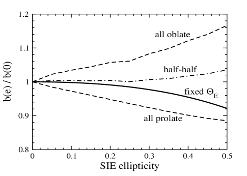
Figure 1.— Change in the isothermal ellipsoid $b$ parameter as a function of ellipticity. The two dashed curves show the dynamical normalization if all halos are assumed to be oblate or prolate. The dot-dashed curve shows the case when half of the halos are assumed to be oblate and half prolate. The solid curve shows the result when the Einstein radius is fixed to be independent of ellipticity, which is what we assume in this paper.

Objects in the vicinity of the lens galaxy create tidal forces that affect the lens potential. The contribution is often modeled as an external shear whose contribution to the lens potential is

$$\Phi_{\rm shear}(r,\phi)=-\frac{\gamma}{2}\,r^{2}\,\cos 2(\phi-\phi_{\gamma})\,,$$ (11)

where $(r,\phi)$ are polar coordinates, $\gamma$ is the dimensionless shear amplitude, and $\phi_{\gamma}$ is the direction of the shear. As an example, consider the shear produced by an isothermal sphere galaxy with Einstein radius $b_{0}$ that lies at polar coordinates $(r_{0},\phi_{0})$ relative to the lens galaxy; the shear amplitude would be $\gamma=b_{0}/(2r_{0})$ and the shear direction would be $\phi_{\gamma}=\phi_{0}$. External shear does not contribute to the local surface mass density, so it does not affect the monopole deflection or the Einstein radius.

2.3. Source luminosity functions

The number density of sources with luminosity between $L$ and $L+dL$ is given by the luminosity function $[d\phi_{\rm src}(L)/dL]\,dL$. The quantity of interest for lens statistics (see eq. (1)) is the cumulative number density of sources brighter than $L$, or

$$\Phi_{\rm src}(L)=\int_{L}^{\infty}{d\phi_{\rm src}(L^{\prime})\over dL^{\prime}}\,dL^{\prime}\,.$$ (12)

We consider model LFs appropriate to both radio and optical surveys.

The simplest model LF is a featureless power law, $\phi_{\rm src}(L)\propto L^{-\beta}$. In this case the biased cross section simplifies to

$$BA=\int_{\rm mult}\mu^{\beta-1}\ d{\vec{\bf u}}\equiv\int\mu^{\beta-1}\ p(\mu)\ d\mu\,,$$ (13)

where $p(\mu)$ is the distribution of magnifications for lensed sources. Several points are worth mentioning. First, with $\beta\to 1^{+}$ the magnification weighting factor becomes unity and we recover the simple lensing cross section with no magnification bias. Second, because the magnification distribution generically has a power law tail $p(\mu)\propto\mu^{-3}$ for $\mu\gg 1$ (see Schneider, Ehlers, & Falco, 1992), the integral diverges for $\beta\geq 3$ and the biased cross section is well defined only for $\beta<3$. Finally, a power law is featureless so the biased cross section does not depend on the particular flux or luminosity limit of a survey. A power law LF is a good model for radio surveys. For example, the largest existing lens survey is the JVAS/CLASS survey of flat-spectrum radio sources (Myers et al., 2003; Browne et al., 2003), and it has an LF that is well described by a power law with $\beta\approx 2.1$ (see Rusin & Tegmark, 2001; Chae, 2003).

Future lens samples are likely to be dominated by optically-selected quasar lenses found in deep wide-field imaging surveys (e.g., Kuhlen et al., 2004). While accurate determination of the quasar LF is a long-standing problem, recent evidence favors the double power law form proposed by Boyle, Shanks, & Peterson (1988),

$${d\phi(L,z)\over dL}\,dL=\frac{\phi_{*}}{[L/L_{*}(z)]^{\beta_{l}}+[L/L_{*}(z)]^{\beta_{h}}}\ \frac{dL}{L_{*}(z)}\ ,$$ (14)

where the break luminosity $L_{*}$ evolves with redshift as (Madau et al., 1999)

$$L_{*}(z)=L_{*}(0)\ (1+z)^{\alpha_{\rm s}-1}\ \frac{e^{\zeta z}(1+e^{\xi z_{*}})}{e^{\xi z}+e^{\xi z_{*}}}\ ,$$ (15)

where the quasar spectral energy distribution is assumed to be a power law, $f_{\nu}\propto\nu^{-\alpha_{\rm s}}$. With this LF, the biased cross section clearly depends on the bright and faint slopes $\beta_{h}$ and $\beta_{l}$, and also on the limiting luminosity $L_{\rm cut}(z)/L_{*}(z)$. It depends on source redshift to the extent that these quantities depend on redshift. We adopt the model from Fan et al. (2001) with bright-end slope $\beta_{h}=3.43$ at $z<3$ and $\beta_{h}=2.58$ at $z>3$, and faint-end slope $\beta_{l}=1.64$ at all redshifts (Wyithe & Loeb, 2002).

If we wanted to compute statistics for real quasar lens surveys, we would need to adopt an appropriate limiting magnitude and compute the limiting luminosity $L_{\rm cut}(z)/L_{*}(z)$ as a function of redshift. This would require specifying the passband, computing $K$-corrections, and other details that would muddy the waters. Since the goal is conceptual understanding of the effects, we believe that it is simpler and more instructive to work with a luminosity cut $L_{\rm cut}/L_{*}$. In this case, we do not need to specify the parameters $\phi_{*}$, $L_{*}(0)$, $z_{*}$, $\zeta$, and $\xi$.

2.4. Numerical techniques

We compute the integrals in eqs. (2)–(5) using Monte Carlo techniques. First, for fixed ellipticity and shear we place $10^{5}$–$10^{6}$ random sources in the source plane, in the smallest circle enclosing the caustics. We solve the lens equation using the gravlens software (Keeton, 2001) to determine the number of images and their positions and magnifications. We define the image separation to be the maximal separation between any two images in the system, $\Delta\theta\equiv\max|\vec{\theta_{i}}-\vec{\theta_{j}}|$; this is a convenient, observable, and well-defined quantity that is independent of the number of images.

We separate the lenses into three standard classes based on the image multiplicity: “doubles” have two bright images, one with positive parity and one negative, plus a faint central image that is rarely observed; “quads” have four bright images, two positive and two negative parity, plus a faint central image that is rarely observed; and “naked cusps” have three bright images, either two positive parity and one negative or vice versa. We use the classifications directly only when studying the quadruple-to- double ratio (§ 5). The classification offers a fringe benefit: we can identify numerical errors as systems that do not fit into any of the classes (because, for example, the software failed to find one of the images). We estimate that the numerical failure rate is $<\!10^{-4}$.

Next, where appropriate we integrate over distributions for ellipticity and shear. For the ellipticity, we adopt the distribution of ellipticities measured for 379 early-type galaxies in 11 nearby clusters by Jørgensen et al. (1995). The distribution has mean $\langle{e}\rangle=0.31$ and dispersion $\sigma_{e}=0.18$, and there are no galaxies with $e\gtrsim 0.8$. Although the measured ellipticities describe the luminosity while what we need for lensing is the ellipticity of the mass distribution, this is probably the best we can do at the moment. In any case, it seems reasonable to think that the ellipticity distributions for the light and the mass may be similar (see Rusin & Tegmark, 2001). For the shear, Holder & Schechter (2003) estimate that the distribution of shear amplitudes derived from simulations of galaxy formation can be described as a lognormal distribution with median $\gamma=0.05$ and dispersion $\sigma_{\gamma}=0.2$ dex; this distribution is also broadly consistent with the shears required to fit observed lenses. As a rule of thumb, a shear $\gamma\sim 0.1$ is common for lenses in poor groups of galaxies, and the shear can reach $\gamma\sim 0.3$ for lenses in rich clusters (e.g., Keeton et al., 1997; Kundić et al., 1997a, b; Fischer et al., 1998; Kneib et al., 2000). We assume random shear orientations.

3. The Optical Depth

Before determining the effects of ellipticity and shear on the lensing optical depth, it is instructive to consider first how they affect the source plane. There is only a small change in the lensing cross section. In fact, for isothermal galaxies shear has no effect on the radial caustic and hence on the cross section. Ellipticity (or any other internal angular structure) in isothermal galaxies changes the caustics in such a way as to reduce the cross section, as explained in the Appendix. The main effect of increasing ellipticity or shear is to lengthen the tangential caustic, which enlarges the phase space for large magnifications and raises the tail of the magnification distribution, as illustrated in Figure 2. In particular, we see a sharp increase in the cross section for producing magnifications larger than the minimum magnification for a quadruple lens (see caption).

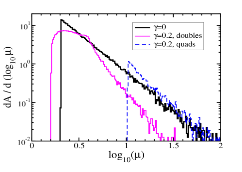
Figure 2.— Magnification distributions for spherical deflectors without shear and with shear $\gamma=0.2$. The curves are normalized so that the area under each curve is the corresponding cross section in units of $\theta_{E}^{2}$. For the shear case we show the distributions for doubles and quadruples separately. Note that the minimum magnification for doubles is $\mu_{2,\rm min}=2/[(1+3\gamma)(1-\gamma)]$, while for quadruples it is $\mu_{4,\rm min}=2/[\gamma(1-\gamma^{2})]$ (Finch et al., 2002); so $\mu_{2,\rm min}=1.56$ and $\mu_{4,\rm min}=10.4$ for the case $\gamma=0.2$ shown here. The distributions asymptote to $A(\mu)\propto\mu^{-3}$ at high magnifications (Schneider et al., 1992).

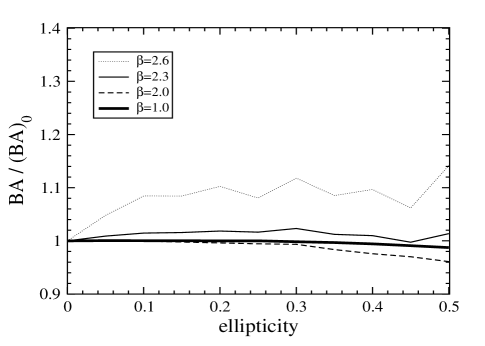
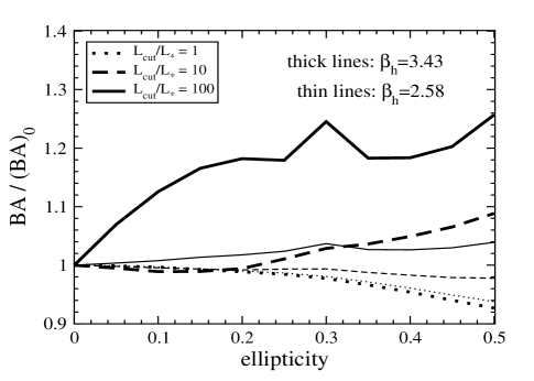
Figure 3.— Enhancement in the biased cross section caused by ellipticity. The shear is set to zero. (a, left) Results for different power law source LFs. Recall that with $\beta\to 1^{+}$ there is no magnification bias, and that the CLASS radio survey has $\beta\approx 2.1$. (b, right) Results for the model quasar LF, for different values of the limiting luminosity ($L_{\rm cut}/L_{*}$) and the bright-end slope ($\beta_{h}$); the faint-end slope is fixed at $\beta_{l}=1.64$. The jaggedness in the upper curves is due to statistical noise, because for steep LFs the magnification bias is strong and the results are dominated by rare extreme-magnification systems. We estimate the statistical errors in the upper curves to be $\sim$3%, and much smaller for the other curves.

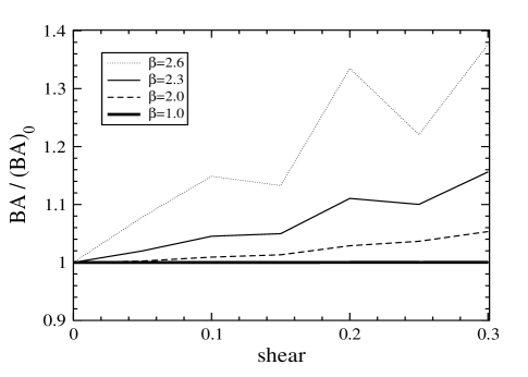
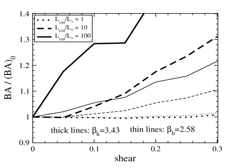
Figure 4.— Similar to Figure 3, but for shear. The ellipticity is set to zero here. The statistical errors in the upper curves are $\sim$10%, and much smaller for the other curves.

We now examine the dependence of the biased cross section $BA$ on ellipticity (Figure 3) and shear (Figure 4). When the LF is a power law with $\beta\to 1^{+}$ there is no magnification bias, and Figure 3 illustrates how ellipticity reduces the cross section. Even with magnification bias, ellipticities up to $e\sim 0.5$ do not affect the biased cross section by more than 10% unless the source LF is very steep (e.g., the very brightest quasars, $L_{\rm cut}/L_{*}\gtrsim 100$ when $\beta_{h}=3.43$). Figure 4 shows that shear causes a stronger increase in the biased cross section, but we must remember that realistic shears are $\gamma\lesssim 0.1$ and only lenses in clusters experience large shears of $\gamma\sim 0.2$–0.3. Thus, the typical change in the biased cross section due to shear is again no more than 10% unless the LF is very steep.

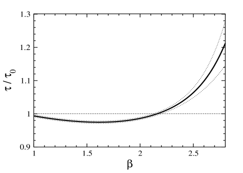
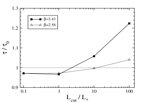
Figure 5.— Enhancement in the optical depth as a function of the luminosity function slope $\beta$ for power law LFs (left) or the limiting luminosity $L_{\rm cut}/L_{*}$ for quasar LFs (right). In the left panel, the solid line shows the fiducial result while the dotted lines indicate the statistical uncertainty from our calculation.

To compute changes in the full optical depth we integrate the biased optical depth over appropriate distributions of ellipticity and shear (see eq. (4)). The results are shown in Figure 5. Without magnification bias ($\beta\to 1^{+}$), ellipticity and shear reduce the optical depth very slightly (by $\sim$0.6%, although the statistical uncertainty from our Monte Carlo calculations is $\sim$0.3%) With magnification bias and a shallow source LF, ellipticity and shear can reduce the optical depth by up to $\sim$2.5% relative to the spherical case. For power law LFs, only when $\beta\geq 2.2$ is there an increase in the optical depth, and we must have $\beta\geq 2.5$ ($\beta\geq 2.6$) in order for the increase to be more than 5% (10%). For the quasar LF, the increase exceeds 5% only if the bright end is steep ($\beta_{h}=3.43$) and the survey is limited to bright quasars ($L_{\rm cut}/L_{*}\gtrsim 10$).

In practice, these results mean that ellipticity and shear are important for the optical depth only in surveys that are restricted to the brightest quasars. They are not very significant for the sorts of deep optical surveys now underway that probe well beyond the break in the quasar LF.

4. The Image Separation Distribution

We now turn to the distribution of lens image separations and how it is affected by ellipticity and shear. First, we recall several basic facts. Even in spherical models the distribution of dimensioned image separations will have some natural spread because of the range of galaxy masses and redshifts; but the distribution of dimensionless separations $\Delta\hat{\theta}$ is a $\delta$-function at $\Delta\hat{\theta}=2$. To highlight changes in the separation distribution, it is therefore useful to focus on the distribution of $\Delta\hat{\theta}$. Also, as discussed in § 2.4, we define the separation to be the maximal distance between any pair of images.

Figure 6 shows the distribution of $\Delta\hat{\theta}$ for several values of ellipticity (upper panel) and shear (lower panel). The distribution has an interesting shape that peaks at the ends and is low in the middle. It has a sharp cutoff at the high end, while at the low end it has a sharp drop followed by a small tail to lower values. The peaks correspond to sources near the minor and major axes of the lens potential.

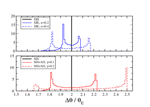
Figure 6.— Histograms of the dimensionless image separation $\Delta\hat{\theta}={\Delta\theta}/\theta_{E}$, for two values of ellipticity (top panel) and shear (bottom). For a spherical lens the distribution is a $\delta$-function at $\Delta\hat{\theta}=2$, indicated by the vertical line. The histograms contain all image multiplicities (i.e., both doubles and quadruples). The results are shown for the CLASS LF (a power law with $\beta=2.1$), but they are not very sensitive to this choice.

As the ellipticity or shear increases, the distribution of $\Delta\hat{\theta}$ broadens and its mean shifts. To quantify these effects, we compute the mean separation $\langle{\Delta\hat{\theta}}\rangle$ and the spread $\sigma_{\Delta\hat{\theta}}=(\langle{\Delta\hat{\theta}^{2}}\rangle-\langle{\Delta\hat{\theta}}\rangle^{2})^{1/2}$, and plot them as a function of ellipticity or shear in Figure 7. The increase in the mean and scatter are small for all ellipticities, and are both $<$20% for all but the strongest shears ($\gamma\gtrsim 0.3$) felt by lenses in cluster environments. Nevertheless, it is interesting that shear produces a net bias toward larger image separations.

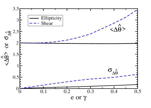
Figure 7.— Mean and spread of the image separation distribution as a function of ellipticity or shear. The image separations are in units of $\theta_{E}$. As in Figure 6, the results are shown for the CLASS LF but are not very sensitive to this choice.

Finally, by averaging over the ellipticity and shear distributions we obtain the net image separation distribution shown in Figure 8. The averaging has smoothed out the sharp features seen in Figure 6 when the ellipticity and shear were fixed. The net distribution is nearly Gaussian, with mean $\Delta\hat{\theta}=2.01$ and scatter $\sigma_{\Delta\hat{\theta}}=0.18$ for a power law LF with $\beta=2.1$, or $\Delta\hat{\theta}\approx 2.01$ and $\sigma_{\Delta\hat{\theta}}\approx 0.19$ for various cases of the quasar LF. In other words, ellipticity and shear basically leave the mean image separation unchanged but create an additional scatter of 10%, and these results are insensitive to the source LF.

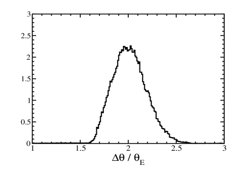
Figure 8.— Net image separation distribution after averaging over ellipticity and shear. The histogram is normalized to unit area. The results are again shown for the CLASS LF but are not very sensitive to this choice. The distribution is nearly Gaussian, with mean $\Delta\hat{\theta}=2.01$ and scatter $\sigma_{\Delta\hat{\theta}}=0.18$.

5. Quadruple-to-Double Ratio

We next consider how ellipticity and shear affect the number of lenses with different image configurations. While an SIS lens always produces two images, increasing ellipticity or shear leads to increasing probability for configurations with four images. Furthermore, large ellipticities ($e>0.606$) or shears ($\gamma>1/3$) can lead to “naked cusp” configurations with three bright images (e.g., Keeton et al., 1997). Nearly all known lenses with point-like images are doubles or quadruples; among $\sim$80 known lenses there is only one candidate naked cusp lens (APM 08279+5255; Lewis et al., 2002).

Figure 9 shows that the quadruple to double ratio rises monotonically with ellipticity or shear. For the CLASS LF, the ratio is $\sim$20% for typical ellipticities $e\sim 0.3$ or shears $\gamma\sim 0.1$. Our results agree well with previous analyses (e.g., Rusin & Tegmark, 2001; Finch et al., 2002).

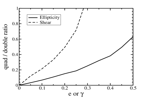
Figure 9.— Quadruple-to-double ratio as a function of ellipticity or shear, assuming the CLASS LF (a power law with $\beta=2.1$).

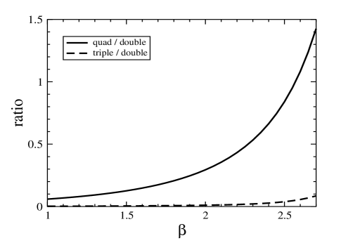
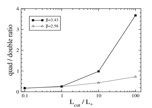
Figure 10.— Quadruple-to-double ratio, as a function of the slope $\beta$ of power law LFs (left) or the limiting luminosity $L_{\rm cut}/L_{*}$ for quasar LFs (right). The results are obtained by averaging over the distributions of ellipticity and shear discussed in the text. In the left panel, we also show the ratio of triple (or naked cusp) lenses as the dashed curve.

We can now estimate the expected number of quadruples (and cusp triples) by averaging over our fiducial distribution of ellipticity and shear. The results are shown in Figure 10 for both the power law LF and the quasar LF. For the CLASS LF ($\beta=2.1$), the net quadruple-to-double ratio is about 0.35, while the triple-to-double ratio is only about 0.01. The number of quadruple vs. double systems in the CLASS statistical sample is 5 vs. 7; the ratio is twice as large as our prediction. We therefore agree with Rusin & Tegmark (2001) in concluding that ellipticity and shear alone cannot easily explain the high number of quadruples. Additional effects are required, which are probably related to lens galaxy environments. Shear is only a low-order approximation to the lensing effects of objects near the lens galaxy. Recent studies have shown that including higher-order effects from satellite galaxies (Cohn & Kochanek, 2003) or extended groups of galaxies (Keeton & Zabludoff, 2004) around the lens can significantly boost the quadruple-to-double ratio.

Figure 10 shows that surveys targeting lensed quasars are expected to have a low quadruple-to-double ratio unless the bright end of the LF is steep ($\beta_{h}=3.43$) and the survey is limited to bright quasars ($L_{\rm cut}/L_{*}\gtrsim 10$). This prediction could, of course, be an underestimate because we have neglected the higher order effects from lens environments.

6. Effects on Cosmological Constraints

While the changes in the optical depth and image separation distribution caused by ellipticity and shear seem mild, it is important to quantify how they affect one of the main applications of lens statistics: constraints on cosmological parameters. One approach would be to modify the analyses of real lens samples to include the full effects of ellipticity and shear (building upon the analysis of Chae 2003). Such an approach, however, would be limited by Poisson uncertainties in current lens samples (e.g., CLASS has just 13 lenses), by systematic uncertainties where models may or may not be correct (e.g., evolution in the lens galaxy population; see Mitchell et al. 2004), and by systematic effects that are known to be present in the data but have not yet been studied (e.g., having multiple lens galaxies). We believe that it is more instructive to create mock lens surveys that mimic CLASS but allow us to isolate the effects of ellipticity and shear. Specifically, we create surveys that include ellipticity and shear, and then analyze them using standard spherical models in order to uncover biases that result from neglecting ellipticity and shear. We create mock surveys with 1000 lenses in order to minimize Poisson uncertainties. We use a Monte Carlo approach, drawing parameter values from appropriate probability distributions (as indicated in eq. 1). Specifically:

• A subset of sources in the CLASS survey has a redshift distribution that can be treated as a Gaussian with mean $\langle{z_{s}}\rangle=1.27$ and width $\sigma_{z}=0.95$ (Marlow et al., 2000), and this is usually taken as a model for the redshift distribution of the full survey (e.g., Chae, 2003). The Gaussian is modified by the redshift dependence of the optical depth $\tau(z_{s})$ to obtain the redshift distribution of the lensed sources (see Mitchell et al., 2004).

• The lens redshift is drawn from the distribution $p(z_{l})\propto(D_{ls}/D_{os})^{2}\ dV/dz_{l}$, where the factor of $(D_{ls}/D_{os})^{2}$ comes from the factor of $\theta_{E}^{2}$ in the lensing cross section (see eq. (10)).

• The velocity dispersion is drawn from $p(\sigma)\propto\sigma^{4}\ dn/d\sigma$, where the factor of $\sigma^{4}$ comes from $\theta_{E}^{2}$ in the lensing cross section. We use the velocity dispersion distribution function $dn/d\sigma$ derived by Sheth et al. (2003) for early-type galaxies in the Sloan Digital Sky Survey. For simplicity, we assume that the velocity dispersion distribution does not evolve with redshift. We could add evolution to both the creation and analysis of the mock survey (see, e.g., Mitchell et al., 2004), but that would just complicate matters.

• We use the ellipticity distribution from Jørgensen et al. (1995), the shear amplitude distribution from Holder & Schechter (2003), and random shear directions.

• When drawing random source positions, we use magnification bias appropriate to the CLASS survey (a power law with $\beta=2.1$) since it is the most commonly used survey in current lens statistic analyses.

Given the parameters we can compute the observables for each mock lens: the source and lens redshifts and the image separation. The other key observable is the total number of sources in the survey. We use the optical depth to determine the number of sources needed to obtain 1000 lenses, which is typically $\sim\!8\times 10^{5}$. We distribute these sources in redshift using the Gaussian given above.

We then analyze the mock survey with standard maximum likelihood techniques. Assuming complete data — knowledge of the image separation and the lens and source redshifts for lens systems, and the redshift distribution of non-lensed sources — we use the likelihood function

$${\cal L}=\frac{(N_{\rm pred})^{N_{\rm obs}}\ e^{-N_{\rm pred}}}{N_{\rm obs}!}\times\prod_{i=1}^{N_{\rm lens}}\frac{1}{\tau(z_{s,i})}\,\frac{\partial^{2}\tau}{\partial z_{l,i}\ \partial{\Delta\theta}_{i}}\ .$$ (16)

The first term represents the Poisson probability for having $N_{\rm obs}$ observed lenses when $N_{\rm pred}$ are predicted, while the second term represents the probability that the lenses have the observed properties (e.g., observed lens redshift $z_{l}$ and image separation ${\Delta\theta}$ given the source redshift $z_{s}$). As mentioned above, we neglect ellipticity and shear in the likelihood analysis because we want to understand the biases that may occur when spherical models are used for lens statistic analyses. We hold the parameters in the velocity dispersion function fixed at their input values since uncertainties in these parameters have negligible effect (Mitchell et al., 2004). Thus, the only variables in the model are the cosmological parameters $\Omega_{M}$ and $\Omega_{\Lambda}$, which we adjust to maximize the likelihood. We use input values of $\Omega_{M}=0.3$ and $\Omega_{\Lambda}=0.7$, and study how much the recovered values differ. As mentioned above, using surveys with 1000 lenses should mitigate Poisson uncertainties, but we always produce and analyze 10 independent surveys to verify that the statistical noise in our results is negligible.

It is useful to begin by examining two toy models that focus on how changes in the optical depth or image separation distribution can affect cosmological constraints. In the first case, we imagine using spherical lens models but manually adjusting the optical depth. This is equivalent to changing the total number of deflectors. In practice, it means adjusting the number of sources in our mock survey (since we fix the number of lenses). The crosses in Figure 11 show the errors in the recovered cosmological parameters if the difference between the actual (input) optical depth and the spherical model is $(-20,-15,-10,-5,0,5,10,15,20)\%$. We see that simply changing the optical depth moves the cosmological parameters mainly along the line corresponding to flat cosmologies, and the shift is fairly small: $\Delta\Omega_{\Lambda}=0.03$ if the real optical depth is 10% larger than predicted by the spherical model.

Figure 11.— Biases in constraints on cosmological parameters from analyses of lens statistics. We show the errors $\Delta\Omega_{M}=\Omega_{M}^{\rm mod}-\Omega_{M}^{\rm true}$ and $\Delta\Omega_{\Lambda}=\Omega_{\Lambda}^{\rm mod}\Omega_{\Lambda}^{\rm true}$ that result from using simple models with spherical lenses that neglect shifts in the optical depth (crosses), image separations (triangles), or both. (See text for details.) The statistical uncertainties are smaller than the size of the points.

In the second case, we again start with spherical models but manually adjust the image separations. This is equivalent to shifting the velocity dispersion distribution to higher or lower values, and then adjusting the number of galaxies to keep the optical depth fixed. The triangles in Figure 11 show the results of shifting the image separations by $(-20,-15,-10,-5,0,5,10,15,20)\%$. There is a large shift in the recovered cosmological parameters, and it is almost orthogonal to the line of flat cosmologies. For example, if the real image separations are 10% larger than predicted by spherical models, then there will be errors of $\Delta\Omega_{M}=0.12$ and $\Delta\Omega_{\Lambda}=0.21$ in the parameters recovered by spherical models. These two cases are just toy examples, but they illustrate the important principle that even small errors in the model image separations can have a significant effect on cosmological constraints (even if small errors in the optical depth do not).

Finally, we consider the case where we use the full effects of ellipticity and shear on the mock survey. Essentially, this amounts to using the corrections to the optical depth from Figure 5 and to the image separation distribution from Figure 8. The circle in Figure 11 shows that neglecting ellipticity and shear in the likelihood analysis causes errors of $\Delta\Omega_{M}=0.00\pm 0.01$ and $\Delta\Omega_{\Lambda}=-0.02\pm 0.01$, where the errorbars represent the statistical uncertainties in our calculations. (We have achieved small Poisson uncertainties but not eliminated them altogether.) That is the case if we allow $\Omega_{M}$ and $\Omega_{\Lambda}$ to vary independently. If we restrict attention to flat cosmologies ($\Omega_{M}+\Omega_{\Lambda}=1$) then the bias is just $\Delta\Omega_{M}=-\Delta\Omega_{\Lambda}=0.01$ (with negligible errorbars). This result is consistent with our conclusions from the previous sections that ellipticity and shear have little effect on the optical depth and mean image separation. It is nonetheless valuable to have a careful validation of the conventional wisdom that ellipticity and shear do not significantly affect cosmological constraints derived from lens statistics.

7. Conclusions

The effects of ellipticity and shear on strong lensing statistics have been swept under the rug in most analyses to date (a valiant exception being Chae 2003). The reason for this is twofold: (1) models with nonspherical deflectors introduce new, and sometimes poorly constrained, parameters and greatly complicate calculations; and (2) conventional wisdom suggested that realistic ellipticities and shears had little effect on anything but the image multiplicities. We have stepped beyond the state of blissful ignorance to present a general analysis of how ellipticity and shear enter into lens statistics.

The effects depend strongly on magnification bias, which in turn depends on the luminosity function of sources in a lens survey. If the LF is a power law $\propto L^{-\beta}$, as in radio surveys like CLASS (with $\beta\approx 2.1$), ellipticity and shear generally decrease or increase the lensing optical depth by only a few percent. The increase is more than 5% only if the LF is steep ($\beta\gtrsim 2.5$). For optical quasar surveys, if the limiting luminosity is below the break in the quasar LF then ellipticity and shear decrease the optical depth by a few percent. There is a noticeable ($>$5%) increase only for surveys limited to the brightest quasars ($L_{\rm cut}/L_{*}\gtrsim 10$, if the bright end slope is $\beta_{h}=3.43$). Since ongoing and planned optical surveys are expected to reach to the faint end of the QSO LF ($L_{\rm cut}/L_{*}\lesssim 1$), we do not expect ellipticity and shear to have a large effect on the predicted number of lenses in future lens surveys.

Ellipticity and shear do not shift the mean of the distribution of lens image separations, but they do introduce an additional scatter of $\sim$10%. They naturally affect the relative numbers of double, quadruple, and triple lenses, but they cannot easily explain the high observed quadruple-to-double ratio. Ellipticity has little effect on predictions for elusive central lensed images, although it does lead to a segregation that quadruple lenses are generally expected to have fainter central images than double lenses (Keeton, 2003).

Since ellipticity and shear produce only small changes in the lensing optical depth and image separation distribution, they are not very important in lensing constraints on cosmological parameters. Neglecting them leads to biases in $\Omega_{M}$ and $\Omega_{\Lambda}$ of $<$0.02. Moreover, hydrodynamical N-body simulations tend to find systems that are more spherical than those in dissipationless simulations (e.g., Kazantzidis et al., 2004). Therefore, the ellipticity effects on lensing statistics found in this paper, while already small, could even be an overestimate.

We conclude that for lens statistics problems other than image multiplicities, ellipticity and shear have surprisingly little effect. Unless percent-level precision is needed, or a survey with a particularly steep LF is being considered, ellipticity and shear can probably be ignored. Their effects will become more important as lens samples grow into the hundreds or thousands and statistical uncertainties plummet (see, e.g., Kuhlen et al., 2004). At that time it will be important to know the distributions of ellipticity and shear, and also to resolve questions about how to normalize the lens models (see § 2.2).

There are systematics besides ellipticity and shear that may affect strong lens statistics. They include mergers and evolution in the deflector population (e.g., Rix et al., 1994; Mao & Kochanek, 1994; Keeton, 2002; Ofek et al., 2003; Chae & Mao, 2003; Mitchell et al., 2004), halo triaxiality (e.g., Oguri & Keeton, 2004) or other complex internal structure (e.g., Möller et al., 2003; Quadri et al., 2003), compound lens galaxies (e.g., Kochanek & Apostolakis, 1988; Möller & Blain, 2001; Cohn & Kochanek, 2003), and lens galaxy environments (e.g., Möller et al., 2002; Keeton & Zabludoff, 2004). In order to bring lens statistics into the realm of precision cosmology, each of these factors must be addressed carefully. We have taken one step in that direction by studying ellipticity and shear, finding that their effects are relatively small and in principle easy to take into account.

Appendix A Why is $A/A_{0}\leq 1$?

In this appendix we derive the cross section for a generalized isothermal lens to explain the result from § 3 that ellipticity reduces the cross section. The lens potential for a generalized isothermal model has the form $\Phi_{\rm iso}(r,\phi)=r\,f(\phi)$ where $f(\phi)$ is an arbitrary function specifying the angular shape. Consider expanding the potential in angular multipoles,

$$\Phi_{\rm iso}(r,\phi)=\theta_{E}\,r\,\left(1-\sum_{m=1}^{\infty}\Bigl{[}a_{m}\cos(m\phi)+b_{m}\sin(m\phi)\Bigr{]}\right),$$ (A1)

where $\theta_{E}$ is the Einstein radius (as defined in § 2.2). The corresponding mass distribution then has the form

$$\kappa_{\rm iso}(r,\phi)=\frac{\theta_{E}}{2r}\left(1+\sum_{m=1}^{\infty}\epsilon_{m}\cos[m(\phi-\phi_{m})]\right),$$ (A2)

where the amplitude $\epsilon_{m}$ and direction $\phi_{m}$ of the mass multipole are given by

$$\epsilon_{m} = (m^{2}-1)\sqrt{a_{m}^{2}+b_{m}^{2}}\ ,$$ (A3)

$$\phi_{m} = \frac{1}{m}\tan^{-1}\frac{b_{m}}{a_{m}}\ .$$ (A4)

In other words, we can think of this model as a multipole expansion of the surface mass density.

The radial caustic — properly termed a pseudo-caustic since a singular isothermal lens does not formally have a radial critical curve (see Evans & Wilkinson, 1998) — can then be written in parametric form as:

$$u_{\rm caus}(\lambda) = -\theta_{E}\left(\cos\lambda+\sum_{m=1}^{\infty}\Bigl{[}(a_{m}\cos m\lambda+b_{m}\sin m\lambda)\cos\lambda+m(a_{m}\sin m\lambda-b_{m}\cos m\lambda)\sin\lambda\Bigr{]}\right)$$ (A5)

$$v_{\rm caus}(\lambda) = -\theta_{E}\left(\sin\lambda+\sum_{m=1}^{\infty}\Bigl{[}(a_{m}\cos m\lambda+b_{m}\sin m\lambda)\sin\lambda-m(a_{m}\sin m\lambda-b_{m}\cos m\lambda)\cos\lambda\Bigr{]}\right)$$ (A6)

Although this form appears complicated, if we collect the two coordinates $u_{\rm caus}$ and $v_{\rm caus}$ into a vector ${\vec{\bf u}}_{\rm caus}$ then we can easily evaluate the area inside the radial caustic:

$$A=\int_{0}^{2\pi}\frac{1}{2}\left[{\vec{\bf u}}_{\rm caus}(\lambda)\times\frac{d{\vec{\bf u}}_{\rm caus}}{d\lambda}\right]d\lambda=\pi\,\theta_{E}^{2}\left[1-\frac{1}{2}\sum_{m=1}^{\infty}(a_{m}^{2}+b_{m}^{2})(m^{2}-1)\right].$$ (A7)

This is the lensing cross section (provided there are no naked cusps). The summand, and hence the sum, is manifestly nonnegative, so the cross section for any nonspherical model is $A<A_{0}\equiv\pi\theta_{E}^{2}$. This result is illustrated in Figure 12 for different multipole terms. It is clear that asphericity deforms the caustics in such a way that the cross section is smaller than for the spherical case.

Figure 12.— Radial caustics for isothermal galaxies with different multipole moments. In each panel, the solid curve shows the caustic for the specified model, while the dotted curve shows the caustic of a spherical model for reference. The order $m$ of the multipole moment increases from top to bottom, and the amplitude $\epsilon_{m}$ increases from left to right.

References

- Boyle et al. (1988) Boyle, B. J., Shanks, T., & Peterson, B. A. 1988, MNRAS, 235, 935
- Browne et al. (2003) Browne, I. W. A., et al. 2003, MNRAS, 341, 13
- Chae (2003) Chae, K.-H. 2003, MNRAS, 346, 746
- Chae et al. (2002) Chae, K.-H. et al. 2002, Phys. Rev. Lett., 89, 051301
- Chae & Mao (2003) Chae, K.-H., & Mao, S. 2003, ApJ, 599, L61
- Cohn et al. (2001) Cohn, J. D., Kochanek, C. S., McLeod, B. A., & Keeton, C. R. 2001, ApJ, 554, 1216
- Cohn & Kochanek (2003) Cohn, J. D., & Kochanek, C. S. 2003, preprint (astro- ph/0306171)
- Comerford et al. (2002) Comerford, J. M., Haiman, Z., & Schaye, J. 2002, ApJ, 580, 63
- Davis et al. (2003) Davis, A. N., Huterer, D., & Krauss, L. M. 2003, MNRAS, 344, 1029
- Dubinski & Carlberg (1991) Dubinski, J., & Carlberg, R. G. 1991, ApJ, 378, 496
- Evans & Wilkinson (1998) Evans, N. W., & Wilkinson, M. I. 1998, MNRAS, 296, 800
- Fan et al. (2001) Fan, X. et al. 2001, AJ, 121, 54
- Finch et al. (2002) Finch, T., Carlivati, L. P., Winn, J. N., & Schechter, P. L. 2002, ApJ, 577, 51
- Fischer et al. (1998) Fischer, P., Schade, D., & Barrientos, L. F. 1998, ApJ, 503, L127
- Franx (1993) Franx, M. 1993, in Galactic Bulges (IAU Symposium 153), ed. H. DeJonghe & H. J. Habing, p. 243
- Fukugita & Turner (1991) Fukugita, M., & Turner, E.L. 1991, MNRAS, 253, 99
- Gerhard et al. (2001) Gerhard, O., Kronawitter, A., Saglia, R. P., & Bender, R. 2001, AJ, 121, 1936
- Holder & Schechter (2003) Holder, G., & Schechter, P. 2003, ApJ, 589, 688
- Huterer & Ma (2004) Huterer, D., & Ma, C.-P. 2004, ApJ, 600, L7
- Jing & Suto (2002) Jing, Y. P.; Suto, Y. 2002, 574, 538
- Jørgensen et al. (1995) Jørgensen, I., Franx, M., & Kjærgaard, P. 1995, MNRAS, 273, 1097
- Kazantzidis et al. (2004) Kazantzidis, S., Kravtsov, A.V., Zentner, A.R., Allgood, B., Nagai, D., & Moore, B. 2004, ApJ, 611, L73
- Kassiola & Kovner (1993) Kassiola, A., & Kovner, I. 1993, ApJ, 417, 459
- Keeton (2001) Keeton, C. R. 2001, astro-ph/0102340
- Keeton (2002) Keeton, C. R. 2002, ApJ, 575, L1
- Keeton (2003) Keeton, C. R. 2003, ApJ, 582, 17
- Keeton et al. (1997) Keeton, C. R., Kochanek, C. S., & Seljak, U. 1997, ApJ, 482, 604
- Keeton & Kochanek (1998) Keeton, C. R., & Kochanek, C. S. 1998, ApJ, 495, 157
- Keeton & Madau (2001) Keeton, C. R., & Madau, P. 2001, ApJ, 549, L25
- Keeton & Zabludoff (2004) Keeton, C. R., & Zabludoff, A. I. 2004, ApJ, submitted
- King & Browne (1996) King, L. J., & Browne, I. W. A., 1996, MNRAS, 282, 67
- Kneib et al. (2000) Kneib, J.-P., Cohen, J. G., & Hjorth, J. 2000, ApJ, 544, L35
- Kochanek (1993a) Kochanek, C. S. 1993a, MNRAS, 261, 453
- Kochanek (1993b) Kochanek, C. S. 1993, ApJ, 419, 12
- Kochanek (1994) Kochanek, C. S. 1994, ApJ, 436, 56
- Kochanek (1995) Kochanek, C. S. 1995, ApJ, 453, 545
- Kochanek (1996a) Kochanek, C. S. 1996a, ApJ, 466, 638
- Kochanek (1996b) Kochanek, C. S. 1996b, ApJ, 473, 595
- Kochanek & Apostolakis (1988) Kochanek, C. S., & Apostolakis, J., 1988, MNRAS, 235, 1073
- Koopmans et al. (2003) Koopmans, L. V. E., Treu, T., Fassnacht, C. D., Blandford, R. D., & Surpi, G. 2003, ApJ, 599, 70
- Kormann et al. (1994) Kormann, R., Schneider, P., & Bartelmann, M. 1994, A&A, 284, 285
- Kuhlen et al. (2004) Kuhlen, M., Keeton, C. R., & Madau, P. 2004, ApJ, 601, 104
- Kundić et al. (1997a) Kundić, T., Cohen, J. G., Blandford, R. D., & Lubin, L. M. 1997a, AJ, 114, 507
- Kundić et al. (1997b) Kundić, T., Hogg, D. W., Blandford, R. D., Cohen, J. G., Lubin, L. M., & Larkin, J. E. 1997b, AJ, 114, 2276
- Lewis et al. (2002) Lewis, G. F., Carilli, C., Papadopoulos, P., & Ivison, R. J. 2002, MNRAS, 330, L15
- Li & Ostriker (2002) Li, L. X., & Ostriker, J. P. 2002, ApJ, 566, 652
- Madau et al. (1999) Madau, P., Haardt, F., & Rees, M. J. 1999, ApJ, 514, 648
- Mao & Kochanek (1994) Mao, S., & Kochanek, C. S. 1994, MNRAS, 268, 569
- Maoz et al. (1997) Maoz, D., Rix, H.-W., Gal-Yam, A., & Gould, A. 1997, ApJ, 486, 75
- Marlow et al. (2000) Marlow, D. R., Rusin, D., Jackson, N., Wilkinson, P. N., & Browne, I. W. A. 2000, AJ, 119, 2629
- Mitchell et al. (2004) Mitchell, J. L., Keeton, C. R., Frieman, J. A., & Sheth, R. K. 2004, ApJ, submitted (astro-ph/0401138)
- Möller & Blain (2001) Möller, O., & Blain, A.W. 2001, MNRAS, 327, 339
- Möller et al. (2002) Möller, O., Natarajan, P., Kneib, J.-P. & Blain, A. W. 2002, ApJ, 573, 562
- Möller et al. (2003) Möller, O., Hewett, P., & Blain, A. W. 2003, MNRAS, 345, 1
- Muñoz et al. (2001) Muñoz, J. A., Kochanek, C. S., & Keeton, C. R. 2001, ApJ, 558, 657
- Myers et al. (2003) Myers, S. T., et al. 2003, MNRAS, 341, 1
- Narayan & White (1988) Narayan, R., & White, S. D. M. 1988, MNRAS, 231, 97P
- Navarro, Frenk, & White (1997) Navarro, J. F., Frenk, C. S., & White, S. D. M. 1997, ApJ, 490, 493
- Ofek et al. (2003) Ofek, E. O., Rix, H. W., & Maoz, D. 2003, MNRAS, 343, 639
- Oguri & Keeton (2004) Oguri, M., & Keeton, C. R. 2004, ApJ, in press (astro- ph/0403633)
- Quadri et al. (2003) Quadri, R., Möller, O. & Natarajan, P., ApJ, 597, 659
- Rix et al. (1994) Rix, H.-W., Maoz, D., Turner, E. L., & Fukugita, M. 1994, ApJ, 435, 49
- Rix et al. (1997) Rix, H.-W., de Zeeuw, P. T., Carollo, C. M., Cretton, N., & van der Marel, R. P. 1997, ApJ, 488, 702
- Rusin et al. (2003) Rusin, D., Kochanek, C. S., & Keeton, C. R. 2003, ApJ, 595, 29
- Rusin & Ma (2001) Rusin, D., & Ma, C.-P. 2001, ApJ, 549, L33
- Rusin & Tegmark (2001) Rusin, D., & Tegmark, M. 2001, ApJ, 553, 709
- Sarbu, Rusin, & Ma (2001) Sarbu, N., Rusin, D. & Ma, C.-P. 2001, ApJ, 561, L147
- Schneider et al. (1992) Schneider, P., Ehlers, J., & Falco, E. E. 1992, Gravitational Lenses (Berlin: Springer-Verlag)
- Sheth et al. (2003) Sheth, R. K., et al. 2003, ApJ, 594, 225
- Takahashi & Chiba (2001) Takahashi, R., & Chiba, T. 2001, ApJ, 563, 489
- Treu & Koopmans (2002) Treu, T., & Koopmans, L. V. E. 2002, ApJ, 575, 87
- Turner et al. (1984) Turner, E. L., Ostriker, J. P., & Gott, J. R. 1984, ApJ, 284, 1
- Witt & Mao (1997) Witt, H. J., & Mao, S. 1997, MNRAS, 291, 211
- Wyithe & Loeb (2002) Wyithe, J. S. B., & Loeb, A. 2002, ApJ, 577, 57
- Zhao (1996) Zhao, H. S. 1996, MNRAS, 278, 488