Spectroscopic source redshifts and parameter constraints from weak lensing and CMB

Abstract

Weak lensing is a potentially robust and model-independent cosmological probe, but its accuracy is dependent on knowledge of the redshift distribution of the source galaxies used. The most robust way to determine the redshift distribution is via spectroscopy of a subsample of the source galaxies. We forecast constraints from combining CMB anisotropies with cosmic shear using a spectroscopically determined redshift distribution, varying the number of spectra $N_{spec}$ obtained from 64 to $\infty$. The source redshift distribution is expanded in a Fourier series, and the amplitudes of each mode are considered as parameters to be constrained via both the spectroscopic and weak lensing data. We assume independent source redshifts, and consider in what circumstances this is a good approximation (the sources are clustered and for narrow spectroscopic surveys with many objects this results in the redshifts being correlated). It is found that for the surveys considered and for a prior of 0.04 on the calibration parameters, the addition of redshift information make significant improvements on the constraints on the cosmological parameters; however, beyond $N_{spec}\sim$few$\times 10^{3}$ the addition of further spectra will make only a very small improvement to the cosmological parameters. We find that a better calibration makes large $N_{spec}$ more useful. Using an eigenvector analysis, we find that the improvement continues with even higher $N_{spec}$, but not in directions that dominate the uncertainties on the standard cosmological parameters.

I Introduction

Weak lensing (WL) is a promising tool for an era of precision cosmology (for reviews, see Refregier (2003); Van Waerbeke and Mellier (2003); Bartelmann and Schneider (2001); Mellier (1999) and references therein). Many recent studies showed the potential of this established technique in constraining various cosmological parameters Hu and Tegmark (1999); Hu (2002); Huterer (2002); Abazajian and Dodelson (2003); Benabed and Van Waerbeke (2003); Takada and Jain (2004); Heavens (2003); Jain and Taylor (2003); Takada and White (2004); Bernstein and Jain (2004); Ishak et al. (2004); Simon et al. (2004). Using current data, Refs. Contaldi et al. (2003); Van Waerbeke et al. (2002); Wang et al. (2003); Jarvis et al. (2003); Massey et al. (2004a) showed that WL can provide constraints that are competitive with other cosmological probes. Many larger and more ambitious surveys are ongoing, planned or proposed. These include the Deep Lens Survey Wittman et al. (2002); the NOAO Deep Survey; the CFHT Legacy Survey Mellier et al. (2001); Pan-STARRS; SNAP Rhodes et al. (2004); Massey et al. (2004b); Refregier et al. (2004); and LSST Tyson (2002). A major challenge for the future of WL studies is to have a very tight control of systematic errors. These include incomplete knowledge of the source redshift distribution Wittman et al. (2000); Refregier (2003). Recent cosmic shear studies have obtained their redshift distributions from joint redshift-magnitude distributions measured in independent surveys Jarvis et al. (2003); from photometric redshifts (“photo-$z$’s”) Brown et al. (2003); or some combination. The former approach suffers from the difficulty that the selection function (and relative weighting) of galaxies may be different in the lensing and redshift surveys, while the latter approach suffers from possible photo-$z$ errors that are difficult to constrain in the absence of spectroscopic confirmation, especially if only a small number of colors are measured. Several studies have marginalized over the source redshift distribution. Ultimately the most robust and model-independent determination of the source redshift distribution would be via spectroscopy of a randomly chosen sub-sample of the source catalog. However, spectroscopy of faint galaxies can be very time-consuming even with today’s large-aperture telescopes. In this paper, we forecast Fisher-matrix constraints from cosmic shear using a spectroscopically determined redshift distribution, varying the number of spectra $N_{spec}$ obtained. The source redshift distribution is expanded in a Fourier series, and the amplitudes of each mode are considered as parameters to be constrained via both the spectroscopic and WL data. We address the effect of galaxy clustering on our analysis and discuss the effect of a better calibration.

II Model parameters

The following basic parameter set for WL is considered: $\Omega_{m}h^{2}$, the physical matter density; $\Omega_{\Lambda}$ and $w$, respectively the fraction of the critical density in a dark energy component and its equation of state; $n_{s}(k_{0}=0.05h/{\rm Mpc})$ and $\alpha_{s}$, the spectral index and running of the primordial scalar power spectrum at $k_{0}$; $\sigma_{8}^{\rm lin}$, the amplitude of linear fluctuations; $\{q_{1}...q_{j_{max}}\}$, the leading coefficients of a Fourier expansion of the source galaxy redshift distribution (see Eq. 4 in the see next section); in the case of two bin tomography we use $\{q_{jA},q_{jB}\}$ with $j=1..j_{\rm max}$. We also include $\zeta_{s}$ and $\zeta_{r}$ as defined in Ishak et al. (2004) to parametrize the shear calibration bias Erben et al. (2001); Bacon et al. (2001); Hirata and Seljak (2003a); Bernstein and Jarvis (2002); Van Waerbeke and Mellier (2003); Kaiser (2000), in which the gravitational shear is systematically over- or under-estimated by a multiplicative factor, i.e. $\hat{P}_{\kappa}(\ell)=(1+\zeta_{s})P_{\kappa}(\ell)$, where $P_{\kappa}(\ell)$ is the convergence power spectrum obtained in the absence of calibration errors. $\zeta_{s}$ refers to the calibration error of the power spectrum, which is twice the calibration error of the amplitude as the power spectrum is proportional to amplitude squared. When we consider tomography, we must also consider the relative calibration $\zeta_{r}$ between the two redshift bins. This error affects the measured power spectrum $\tilde{P}_{\kappa}(\ell)$ in accordance with:

$$\tilde{P}_{\kappa}^{AA}= \!\!\!\!(1+f_{B}\zeta_{r})\hat{P}_{\kappa}^{AA}(\ell),$$

$$\tilde{P}_{\kappa}^{AB}= \!\!\!\!(1+{f_{B}-f_{A}\over 2}\zeta_{r})\hat{P}_{\kappa}^{AB}(\ell),$$

$$\tilde{P}_{\kappa}^{BB}= \!\!\!\!(1-f_{A}\zeta_{r})\hat{P}_{\kappa}^{BB}(\ell),$$ (1)

where $f_{A}$ and $f_{B}$ are the fraction of the source galaxies in bin A and B respectively.

In order to combine this with information from the CMB we include $\Omega_{b}h^{2}$, the physical baryon density; $\tau$, the optical depth to reionization; and $T/S$, the tensor-to-scalar fluctuation ratio. We assume a spatially flat Universe with $\Omega_{m}+\Omega_{\Lambda}=1$, thereby fixing $\Omega_{m}$ and $H_{0}$ as functions of our basic parameters, and we do not include massive neutrinos, or primordial isocurvature perturbations. We use as fiducial model (e.g. Ref. Spergel et al. (2003), with $w$ and $T/S$ added): $\Omega_{b}h^{2}=0.0224$, $\Omega_{m}h^{2}=0.135$, $\Omega_{\Lambda}=0.73$, $w=-1.0$, $n_{s}=0.93$, $\alpha_{s}=0.0$, $\sigma_{8}=0.84$, $\tau=0.17$, $T/S=0.2$, $\zeta_{s}=0.0$, $\zeta_{r}=0.0$, and $q_{i},q_{jA},q_{jB}=0.0$.

We will consider surveys with $f_{sky}=0.01$ and $0.1$, and have number density-to-shape noise ratio $\bar{n}/\langle\gamma^{2}_{int}\rangle=4.1\times 10^{9}$ sr^-1, corresponding to a number density of $\bar{n}=30$ galaxies/arcmin² and shape+measurement noise $\langle\gamma^{2}_{int}\rangle=(0.3)^{2}$. (Note that this is the shape noise in the shear $\gamma$, rather than the ellipticity which is roughly $e\approx 2\gamma$ if isophotal or adaptive ellipticities are used Bernstein and Jarvis (2002); Song and Knox (2004).)

III Parametrization of the redshift distribution

The source averaged distance ratio appears as a weighting function in the convergence power spectrum Kaiser (1992); Jain and Seljak (1997); Kaiser (1998) and is given by

$$g(\chi)=\int_{\chi}^{\chi_{H}}n(\chi^{\prime}){\sin_{K}(\chi^{\prime}-\chi)\over\sin_{K}(\chi^{\prime})}d\chi^{\prime},$$ (2)

where $n(\chi(z))$ is the normalized source redshift distribution. Deviations from the fiducial distribution, Wittman et al. (2000),

$$n_{0}(z)=\frac{z^{2}}{2z_{0}^{3}}\,e^{-z/z_{0}},$$ (3)

(which peaks at $z_{p}=2z_{0}=0.70$ and has $z_{med}\approx 0.94$ ) are parameterized via a Fourier series,

$$n(z)=n_{0}(z)\Big{[}1+\frac{1}{\sqrt{2}}\sum_{j=1}^{\infty}q_{j}\cos(j\pi P_{0}(z))\Big{]},$$ (4)

where $P_{0}$ is the cumulative redshift distribution in the fiducial model,

$$P_{0}(z)=1-\Big{(}1+\frac{z}{z_{0}}+\frac{z^{2}}{2z_{0}^{2}}\Big{)}e^{-z/z_{0}}=\int_{0}^{z}n_{0}(z^{\prime})dz^{\prime}.$$ (5)

The $\{q_{j}\}$ are thus the coefficients in the Fourier expansion of $n(z)/n_{0}(z)$ in the interval $0\leq P_{0}<1$. We have used the cumulative fiducial probability $P_{0}(z)$ instead of $z$ as the independent variable because this will result in uncorrelated constraints on the $q_{j}$ from spectroscopy; the $j=0$ coefficient vanishes because of the normalization constraint $\int n(z)dz=\int n_{0}(z)dz=1$. The selection of the cosines is arbitrary and any complete set of orthogonal functions would work just as well. The distribution is completely specified by the $\{q_{j}\}_{j=1}^{\infty}$, although in this paper we cut off the series at some $j_{\rm max}$ (we show results for $5$ and $100$). For tomography, the normalized distributions and the respective Fourier expansions are given as above, except for bin A we replace $n_{0}(z)$ with

$${n_{0}^{A}(z)=\frac{n_{0}(z)}{1-5/e^{2}}} {\;\;{\rm for}\;\;}{z_{p}\leq 2z_{0}},$$

$${n_{0}^{A}(z)=0} \;\;{\rm for}\;\;{z_{p}>2z_{0}},$$ (6)

and for bin B, we replace $n_{0}(z)$ with

$${n_{0}^{B}(z)=0} \;\;{\rm for}\;\;{z_{p}\leq 2z_{0}},$$

$${n_{0}^{B}(z)=\frac{n_{0}(z)}{5/e^{2}}} {\;\;{\rm for}\;\;}{z_{p}>2z_{0}}.$$ (7)

The cumulative probabilities for the two bins are $P_{0}^{A}(z)=\int_{0}^{z}n_{0}^{A}(z^{\prime})dz^{\prime}$ and $P_{0}^{B}(z)=\int_{0}^{z}n_{0}^{B}(z^{\prime})dz^{\prime}$. We use the parameters $\{q_{1}..q_{5},q_{1}^{A}..q_{5}^{A},q_{1}^{B}..q_{5}^{B}\}$ to vary the redshift distribution, see Fig. 1.

Figure 1: Variations of the redshift distribution. The fiducial distribution $n_{0}(z)$ (which peaks at $z_{p}=2z_{0}$) and the Fourier expansion terms are plotted. The distributions $n_{1\pm}(z)$ represent $q_{1}$ varied by $\pm 25\%$. We also plot $n_{2+}(z)$ to $n_{5+}(z)$. While we varied the $q_{j}^{\prime}s$ by $\pm 0.05$ in the analysis, we plot the $25\%$ variations just for the clarity of the plot.

IV Fisher-matrix analysis

The statistical error on a given parameter $p^{\alpha}$ is given by

$$\sigma^{2}(p^{\alpha})\approx[({\bf F}_{CMB}+{\bf F}_{WL}+{\bf F}_{spec}+\Pi)^{-1}]^{\alpha\alpha},$$ (8)

where $\Pi$ is the prior curvature matrix, and ${\bf F}_{CMB}$, ${\bf F}_{WL}$ and ${\bf F}_{spec}$ are the Fisher matrices from CMB, WL, and spectroscopy, respectively. We use for ${\bf F}_{WL}$ the approach described in Ref. Ishak et al. (2004), with a cutoff at $\ell_{\rm max}=3000$ since on smaller scales the trispectrum contribution to the WL covariance (neglected in Eq. 8) dominates Jain et al. (2000); Cooray and Hu (2001). For CMB, we use the 4 year WMAP parameter constraints including $TT$, $TE$, and $EE$ power spectra, assuming $f_{sky}=0.768$ (the Kp0 mask of Ref. Bennett et al. (2003)), temperature noise of $400$, $480$, and $580\,\mu$K arcmin in Q, V, and W bands respectively (the rms noise was multiplied by $\sqrt{2}$ for polarization), and the beam transfer functions of Ref. Page et al. (2003). The spectroscopy Fisher matrix is obtained as follows. If a galaxy is chosen at random from the lensing catalog, and is spectroscopically determined to have redshift $z$, then the log-likelihood for the redshift distribution parameters $q_{j}$ is

$$\ln{\cal L}(q_{j})=\ln n_{0}(z)+\ln\Big{[}1+{1\over\sqrt{2}}\sum_{j}q_{j}\cos(j\pi P_{0}(z))\Big{]}.$$ (9)

The contribution to the Fisher matrix from this single galaxy is

$$F^{(1)}_{spec}(q_{j},q_{k})\! = \Big{\langle}{\partial\ln{\cal L}\over\partial q_{j}}{\partial\ln{\cal L}\over\partial q_{k}}\Big{\rangle}$$ (10)

$$= \Big{\langle}\frac{\cos(j\pi P_{0}(z))\cos(k\pi P_{0}(z))}{2}\Big{\rangle}=\frac{\delta_{jk}}{4}.\;\;$$

The last equality follows from the orthonormality of the Fourier modes, combined with the fact that $P_{0}(z)$ is uniformly distributed between $0$ and $1$. If $N_{spec}$ galaxies have their spectra measured, and these galaxies are drawn independently from the source catalog, then the above Fisher matrix is multiplied by $N_{spec}$:

$$F^{(N_{spec})}_{spec}(q_{j},q_{k})={1\over 4}N_{spec}\delta_{jk}.$$ (11)

In the case of tomography, we have only $N_{spec}/2$ spectra in each of the two tomography bins $A$ and $B$, and so:

$$F^{(N_{spec})}_{spec}(q_{j}^{A},q_{k}^{A})={1\over 8}N_{spec}\delta_{jk},$$ (12)

and similarly for bin $B$. In principle it is possible to take different numbers of spectra in the two bins; we have not attempted any optimization of this. We consider the cases of $N_{spec}=0$, $64$, $512$ and $4096$ respectively. The results can be compared to the case where the source redshift distribution is known exactly by taking the limit $N_{spec}\rightarrow\infty$.

The Fisher matrix is an asymptotic expansion, and while it is the standard tool of parameter forecasting, it sometimes leads to over-optimistic parameter constraints (see Ref. Hirata and Seljak (2003b) for an extreme example). We have not tested its validity when used with this many parameters, although this could be done by Monte Carlo methods as used by Ref. Tereno et al. (2004).

V Spectroscopy

In the discussion above, it has been assumed that the spectroscopically obtained $n(z)$ is on average the same as the redshift distribution $n(z)$ of the sources used for lensing, and that the redshifts of the galaxies targeted for spectroscopy are independent. These assumptions will be literally true in the idealized case that the spectroscopic galaxies are chosen independently from the lensing source catalog, and there are no failures to obtain spectro-$z$’s. In practice, spectro-$z$s would probably be obtained by a multi-object spectrograph attached to a large telescope. The spectro-$z$ failure rate will be minimized by using the longest practical integration time to maximize signal-to-noise for each spectrum, and the demands on telescope time are thus reduced if multiple objects in the same field of view can be targeted simultaneously. However in this case the galaxies are not being drawn independently from the source catalog, in particular large-scale clustering can cause the redshifts of neighboring source galaxies to become correlated. The feasibility of obtaining many independent spectro-$z$’s is directly tied to the clustering of the sources and the field of view of the telescope since these determine the maximum number of galaxies that can be simultaneously targeted for spectroscopy without the results being strongly correlated.

The effect of source clustering can be understood within the context of Fisher matrix theory as follows. If the fiducial model is correct, and the analysis is done assuming that the spectro-$z$s are independent, the difference $\delta p^{\alpha}=p^{\alpha}({\rm est})-p^{\alpha}({\rm fid})$ between the estimated and fiducial model parameters is roughly

$$\delta p^{\alpha}\approx[{\bf F}^{-1}]^{\alpha\beta}\left.{\partial\ln{\cal L}\over\partial p^{\beta}}\right|_{\rm fid},$$ (13)

where ${\cal L}$ is the likelihood assuming independent spectro-$z$s (i.e. the sum of Eq. 9 over the spectroscopic targets), ${\bf F}$ is the Fisher matrix (also assuming independent spectro-$z$s), and the gradient is taken at the fiducial model. So long as each galaxy in the lensing source catalog has an equal probability of being targeted for spectroscopy, it is easy to see that the spectroscopy contribution to $\langle{\partial\ln{\cal L}\over\partial q_{j}}\rangle=\frac{1}{\sqrt{2}}\sum_{a=1}^{N_{spec}}\langle\cos(j\pi P_{0}(z_{a}))\rangle=0$ and hence $\langle\delta p^{\alpha}\rangle=0$, i.e. the inclusion of the spectroscopy likelihood function introduces no bias in the parameters even if the spectroscopic galaxies are not chosen independently. However, the clustering of the sources does increase the covariance matrix of the $\delta p^{\alpha}$; taking the covariance of Eq. (13) gives

$$\langle\delta p^{\alpha}\delta p^{\beta}\rangle \approx [{\bf F}^{-1}]^{\alpha\gamma}[{\bf F}^{-1}]^{\beta\delta}\left\langle{\partial\ln{\cal L}\over\partial p^{\gamma}}{\partial\ln{\cal L}\over\partial p^{\delta}}\right\rangle_{\rm fid}$$ (14)

$$= [{\bf F}^{-1}]^{\alpha\gamma}[{\bf F}^{-1}]^{\beta\delta}\Bigl{\{}[{\bf F}_{CMB}+{\bf F}_{WL}+\Pi]_{\gamma\delta}$$

$$+\delta_{\gamma}^{q_{j}}\delta_{\delta}^{q_{k}}\sum_{a,b=1}^{N_{spec}}\frac{\langle\cos(j\pi P_{0}(z_{a}))\cos(k\pi P_{0}(z_{b}))\rangle}{2}\Bigr{\}}.$$

If we included only the $a=b$ terms in Eq. (14), the last term in $\{\}$ would simply be the spectroscopy Fisher matrix for independent spectro-$z$s, $F_{spec,\gamma\delta}$. The $a\neq b$ terms are only non-zero due to correlations of the galaxies with each other, and they contribute to quantity in $\{\}$ by an amount $\Delta_{q_{j}q_{k}}$. Since the probability of two galaxies separated by angle $\theta_{ab}$ being physically associated with each other is $\omega(\theta_{ab})/[1+\omega(\theta_{ab})]$, where $\omega$ is the angular correlation function, and the cosine is bounded in the range $-1$ to $+1$, it follows that the $a\neq b$ contribution is

$$|\Delta_{q_{j}q_{k}}|\leq{1\over 2}\sum_{a\neq b}\frac{\omega(\theta_{ab})}{1+\omega(\theta_{ab})}\leq{1\over 2}\sum_{a\neq b}\omega(\theta_{ab}),$$ (15)

as compared with $F_{spec,q_{j}q_{k}}={1\over 4}N_{spec}\delta_{jk}$. Therefore if $\sum_{a\neq b}\omega(\theta_{ab})\ll N_{spec}/2$, then the clustering contribution $\Delta_{\gamma\delta}$ will be small compared to the spectroscopy Fisher matrix $F_{spec,\gamma\delta}$ and hence will contribute negligibly to the parameter uncertainties according to Eq. (14).

Let us consider the implications of this result for an idealized spectroscopic survey strategy that consists of observing $J$ widely separated fields, and obtaining $M=N_{spec}/J$ spectra in each field. We suppose the telescope has a circular field of view of angular radius $r$, that the number density of galaxies targeted for selection in each field is $n=M/\pi r^{2}$, and that the angular correlation function is $\omega(\theta)=(\theta_{0}/\theta)^{0.7}$. We then have

$$\sum_{a\neq b}\omega(\theta_{ab}) \approx n^{2}J\int\int\left(\frac{\theta_{0}}{|\vec{\theta}_{1}-\vec{\theta}_{2}|}\right)^{0.7}\,d\vec{\theta}_{1}\,d\vec{\theta}_{2}$$ (16)

$$= 13.25\,n^{2}J\theta_{0}^{0.7}r^{3.3}=1.34\,{N_{spec}^{2}\over J}\left({\theta_{0}\over r}\right)^{0.7}.$$

where the integrals are taken over a circular disk of radius $r$. (The replacement of the galaxy-galaxy pair summation by an integral is appropriate because the integral is convergent at small separation $|\vec{\theta}_{1}-\vec{\theta}_{2}|$.) The factor of $J$ in the first line occurs because we have to repeat the sum for each of the $J$ fields. In order to have $\sum_{a\neq b}\omega(\theta_{ab})\ll N_{spec}/2$, Eq. (16) tells us that we need a number of fields given by

$$J\gg 2.68\,N_{spec}\left({\theta_{0}\over r}\right)^{0.7}.$$ (17)

Not surprisingly, the number of fields that need to be observed depends on the ratio of the field-of-view radius $r$ to the angular clustering scale $\theta_{0}$. An angular clustering scale of $\theta_{0}\sim 0.0002$ degrees is observed in SDSS Connolly et al. (2002) for the magnitude range $21<r<22$ (valid at separations of 1–30 arcmin). Even smaller $\theta_{0}$ applies to fainter samples, e.g. the CFDF survey McCracken et al. (2001) finds $\omega(1^{\prime})\approx 0.01$ for $18.5<I_{AB}<25$ galaxies, corresponding to $\theta_{0}=2.3\times 10^{-5}$ degrees (for slope $-0.7$, which is consistent with the $\omega(\theta)$ data from $<1$ to several arcminutes). The fainter CFDF sample is probably more representative of the galaxies that will be used in future WL surveys. For $N_{spec}=512$ and a field of view of 0.5 degree radius, we find from Eq. (17) the requirement $J\gg 6$ ($\theta_{0}=0.0002$ deg) or $J\gg 1.3$ ($\theta_{0}=2.3\times 10^{-5}$ deg). In either case the number of fields that must be observed to achieve $N_{spec}=512$ ranges from a few to a few dozen, and for $N_{spec}=4096$ we find that the minimum number of fields $J$ is a few dozen to a few hundred. The number of spectra to be obtained per field is $M=N_{spec}/J\leq\sim 100$.

The problem of spectro-$z$ failures is more difficult to assess than the source clustering. In order to accurately reproduce the $n(z)$ of the lensing source catalog, the targets in the associated spectroscopic survey must be selected randomly from the lensing catalog, or at least have the same selection criteria. Spectro-$z$ failures are not part of the lensing catalog selection criteria, and hence can bias the $n(z)$ determination. The spectro-$z$ failure rate can be reduced by using large-aperture telescopes and very long integration times, which may prove feasible if $r$ is large, $\theta_{0}$ is small, and hence the number of fields $J$ to be observed is only a few. It may also be possible to reduce failures by imposing appropriate color cuts on the source sample. Nevertheless, the failure rate will never be exactly zero. The treatment of systematic errors in $n(z)$ due to these failures is beyond the scope of this paper, but clearly deserves consideration in future work.

VI Results

Table 1: Parameter estimation errors for WL+CMB: For WL, no-tomography, $f_{sky}=0.01,\;0.1$, and $\ell_{\rm max}=3000$. We use $N_{spec}=0$, 64, 512, 4096 and the limit $N_{spec}\rightarrow\infty$, and a priors of 0.04 on $\zeta_{s}$ and $\zeta_{r}$ (unless indicated fixed). In the last part of the table, we show the results with the number of terms in the series increased from 5 to a 100.

	$f_{sky}$	$\Omega_{m}h^{2}$	$\Omega_{b}h^{2}$	$\Omega_{\Lambda}$	$\sigma_{8}$	$n_{s}$	$\alpha_{s}$	$\tau$	$T/S$	$w$	$q_{1}$	$q_{2}$	$q_{3}$	$q_{4}$	$q_{5}$	$\sigma(\zeta_{s})$	$\sigma(\zeta_{r})$
CMB only$\rightarrow$		0.0118	0.0013	0.1981	0.086	0.059	0.036	0.018	0.187	0.872	-	-	-	-	-	-	-
$N_{spec}$=0	0.01	0.0096	0.0009	0.1320	0.053	0.033	0.017	0.018	0.142	0.514	4.342	19.912	34.086	66.902	58.275	0.040	0.040
	0.10	0.0092	0.0009	0.0895	0.039	0.027	0.012	0.018	0.129	0.373	1.595	6.482	13.804	21.929	18.556	0.040	0.040
$N_{spec}$=64	0.01	0.0083	0.0008	0.0248	0.022	0.022	0.012	0.017	0.120	0.226	0.162	0.244	0.250	0.249	0.250	0.040	0.040
	0.10	0.0075	0.0007	0.0141	0.018	0.019	0.010	0.017	0.114	0.186	0.121	0.218	0.249	0.248	0.250	0.040	0.039
$N_{spec}$=512	0.01	0.0076	0.0008	0.0219	0.021	0.021	0.011	0.016	0.115	0.220	0.081	0.088	0.088	0.088	0.088	0.040	0.039
	0.10	0.0058	0.0007	0.0116	0.014	0.016	0.010	0.015	0.098	0.140	0.074	0.087	0.088	0.088	0.088	0.039	0.038
$N_{spec}$=4096	0.01	0.0075	0.0007	0.0211	0.021	0.021	0.011	0.016	0.114	0.219	0.031	0.031	0.031	0.031	0.031	0.040	0.039
	0.10	0.0049	0.0006	0.0111	0.013	0.014	0.009	0.015	0.090	0.118	0.030	0.031	0.031	0.031	0.031	0.039	0.038
$N_{spec}\rightarrow\infty$	0.01	0.0074	0.0007	0.0210	0.021	0.020	0.011	0.016	0.113	0.219	-	-	-	-	-	0.040	0.039
	0.10	0.0047	0.0006	0.0110	0.012	0.013	0.009	0.015	0.088	0.113	-	-	-	-	-	0.039	0.038
$N_{spec}$=0	0.01	0.0096	0.0009	0.1320	0.053	0.033	0.017	0.018	0.142	0.514	4.341	19.912	34.086	66.902	58.275	-	-
$\zeta_{s,r}\;$fixed	0.10	0.0092	0.0009	0.0895	0.039	0.027	0.012	0.018	0.129	0.373	1.594	6.482	13.804	21.928	18.555	-	-
$N_{spec}$=64	0.01	0.0083	0.0008	0.0243	0.022	0.022	0.012	0.017	0.120	0.226	0.159	0.244	0.250	0.249	0.250	-	-
$\zeta_{s,r}\;$fixed	0.10	0.0075	0.0007	0.0137	0.018	0.019	0.010	0.017	0.114	0.185	0.114	0.217	0.249	0.248	0.250	-	-
$N_{spec}$=512	0.01	0.0076	0.0008	0.0211	0.021	0.021	0.011	0.016	0.115	0.220	0.081	0.088	0.088	0.088	0.088	-	-
$\zeta_{s,r}\;$fixed	0.10	0.0056	0.0007	0.0110	0.014	0.015	0.009	0.015	0.096	0.137	0.073	0.087	0.088	0.088	0.088	-	-
$N_{spec}$=4096	0.01	0.0074	0.0007	0.0202	0.021	0.020	0.011	0.016	0.113	0.219	0.031	0.031	0.031	0.031	0.031	-	-
$\zeta_{s,r}\;$fixed	0.10	0.0045	0.0006	0.0105	0.012	0.013	0.009	0.014	0.085	0.110	0.030	0.031	0.031	0.031	0.031	-	-
$N_{spec}\rightarrow\infty$	0.01	0.0073	0.0007	0.0201	0.021	0.020	0.011	0.016	0.113	0.218	-	-	-	-	-	-	-
$\zeta_{s,r}\;$fixed	0.10	0.0042	0.0006	0.0104	0.012	0.012	0.009	0.014	0.083	0.104	-	-	-	-	-	-	-
	$f_{sky}$	$\Omega_{m}h^{2}$	$\Omega_{b}h^{2}$	$\Omega_{\Lambda}$	$\sigma_{8}$	$n_{s}$	$\alpha_{s}$	$\tau$	$T/S$	$w$	$q_{1}$	$q_{2}$	to	$q_{99}$	$q_{100}$	$\sigma(\zeta_{s})$	$\sigma(\zeta_{r})$
$N_{spec}$=64	0.01	0.0083	0.0008	0.0249	0.022	0.022	0.012	0.017	0.120	0.227	0.162	0.244	…	0.250	0.250	0.040	0.040
	0.10	0.0075	0.0007	0.0144	0.018	0.019	0.010	0.017	0.114	0.186	0.122	0.218	…	0.250	0.250	0.040	0.039
$N_{spec}$=512	0.01	0.0076	0.0008	0.0219	0.021	0.021	0.011	0.016	0.115	0.220	0.081	0.088	…	0.088	0.088	0.040	0.039
	0.10	0.0058	0.0007	0.0116	0.014	0.016	0.010	0.015	0.098	0.140	0.074	0.087	…	0.088	0.088	0.039	0.038
$N_{spec}$=4096	0.01	0.0075	0.0007	0.0211	0.021	0.021	0.011	0.016	0.114	0.219	0.031	0.031	…	0.031	0.031	0.040	0.039
	0.10	0.0049	0.0006	0.0111	0.013	0.014	0.009	0.015	0.090	0.118	0.030	0.031	…	0.031	0.031	0.039	0.038
$N_{spec}\rightarrow\infty$	0.01	0.0074	0.0007	0.0210	0.021	0.020	0.011	0.016	0.113	0.219	-	-	…	-	-	0.040	0.039
	0.10	0.0047	0.0006	0.0110	0.012	0.013	0.009	0.015	0.088	0.113	-	-	…	-	-	0.039	0.038

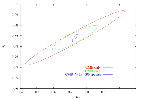
Figure 2: The 68.3% confidence ellipses (assuming Fisher errors) for CMB and weak lensing. Note the improvement in the constraints when spectra are available, versus the case where we marginalize over the redshift distribution parameters.

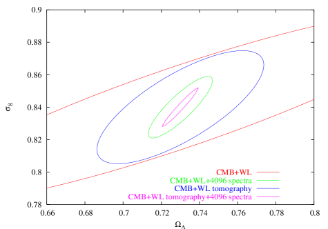
Figure 3: Same as Fig. 2, but including tomography.

Table 2: Parameter estimation errors for WL+CMB: WL $f_{sky}$ is varied from 0.01 to 0.1, and $\ell_{\rm max}=3000$. We use $N_{spec}=0$, 64, 512, 4096 and the limit $N_{spec}\rightarrow\infty$, and priors of 0.04 on $\zeta_{s}$ and $\zeta_{r}$ (unless indicated fixed). Tomgraphy case.

	$f_{sky}$	$\Omega_{\Lambda}$	$\sigma_{8}$	$w$
CMB only$\rightarrow$		0.1981	0.086	0.872
$N_{spec}=0$	0.01	0.0785	0.035	0.339
	0.10	0.0340	0.024	0.240
$N_{spec}=64$	0.01	0.0169	0.018	0.185
	0.10	0.0102	0.013	0.118
$N_{spec}=512$	0.01	0.0160	0.017	0.173
	0.10	0.0084	0.010	0.088
$N_{spec}=4096$	0.01	0.0154	0.016	0.162
	0.10	0.0078	0.009	0.074
$N_{spec}\rightarrow\infty$	0.01	0.0148	0.015	0.154
	0.10	0.0071	0.008	0.066
$N_{spec}=0$	0.01	0.0684	0.032	0.311
$\zeta_{s,r}\;$fixed	0.10	0.0288	0.023	0.230
$N_{spec}=64$	0.01	0.0147	0.017	0.168
$\zeta_{s,r}\;$fixed	0.10	0.0091	0.012	0.108
$N_{spec}=512$	0.01	0.0137	0.016	0.153
$\zeta_{s,r}\;$fixed	0.10	0.0069	0.009	0.075
$N_{spec}=4096$	0.01	0.0130	0.014	0.140
$\zeta_{s,r}\;$fixed	0.10	0.0062	0.008	0.063
$N_{spec}\rightarrow\infty$	0.01	0.0118	0.012	0.122
$\zeta_{s,r}\;$fixed	0.10	0.0043	0.005	0.043

Our results are summarized in Tables 1 and 2, and Figs. 2 and 3. As expected, we find that combination of constraints from WL and from CMB leads to significant improvements in parameter estimation, notably for $\sigma_{8}$, $\Omega_{m}h^{2}$, $n_{s}$, $\alpha_{s}$, $w$ and $\Omega_{\Lambda}$.

As shown in Table 1, the increase of the number of expansion terms from $j_{max}=5$ to 100 has little effect on this result. This suggests that the parameter estimates have converged and, since Eq. (4) can model an arbitrary function for sufficiently large $j_{max}$, it suggests that the form (Eq. 4) for the redshift distribution is not artificially constraining the cosmological parameters.

VII Discussion

In agreement with previous results, we find that the addition of redshift information is helpful for several of the cosmological parameters such as $\Omega_{\Lambda}$, $\sigma_{8}$, $n_{s}$, and $w$. The optical depth $\tau$ is less improved by lensing because most of the statistical power on $\tau$ is coming from the CMB polarization reionization peak, which is not degenerate with any lensing-related quantities. The baryon density is well-constrained by the CMB, however by improving our constraints on several cosmological parameters, lensing information breaks the relatively weak remaining degeneracies in the CMB and reduces the error from $\sigma(\Omega_{b}h^{2})=0.0013$ to $0.0009$. Even lensing with $N_{spec}=0$ is sufficient to break this degeneracy, so inclusion of redshift information adds little for $\Omega_{b}h^{2}$.

The addition of redshift information leads to further significant improvements in the parameter estimation as expected. The $N_{spec}=0$ constraints are substantially worse than $N_{spec}=64$, because in the $N_{spec}=0$ case even wildly oscillating redshift distributions $n(z)$ are formally allowed, as is evidenced by the large $\sigma(q_{j})\gg 1$ in Table 1. Although the gradual addition of spectroscopic redshifts does make additional improvements on the constraints on the cosmological parameters, we find that there is a certain number of $N_{spec}$ (several thousands for the surveys considered here) beyond which the addition of further spectra will make only a very small improvement to the cosmological parameters.

In order to try to explain this, let us recall that error bars are correlated, and hence there can still be combinations of parameters that are degraded by incomplete knowledge of the source redshift distribution. Information on this degradation is contained within the $9\times 9$ covariance matrix C of the cosmological parameters $\{\Omega_{m}h^{2},\Omega_{b}h^{2},\Omega_{\Lambda},\sigma_{8},n_{s},\alpha_{s},\tau,T/S,w\}$. We examine the degradation factor $R$ of the combination of parameters $x=k_{\alpha}p^{\alpha}$ given by

$$R(x)=\frac{\sigma^{2}(x;N_{spec})}{\sigma^{2}(x,N_{spec}=\infty)}=\frac{[\textbf{C}(N_{spec})]^{\alpha\beta}k_{\alpha}k_{\beta}}{[\textbf{C}(\infty)]^{\alpha\beta}k_{\alpha}k_{\beta}}.$$ (18)

The maximum value of $R$ can be found by setting $\partial R/\partial k_{\alpha}=0$, which leads to the eigenvalue equation

$$\frac{[\textbf{C}(N_{spec})]^{\alpha\beta}k_{\alpha}k_{\beta}}{[\textbf{C}(\infty)]^{\alpha\beta}k_{\alpha}k_{\beta}}k_{\gamma}=[\textbf{C}^{-1}(\infty)]_{\gamma\beta}[\textbf{C}(N_{spec})]^{\beta\alpha}k_{\alpha}.$$ (19)

Thus the $k_{\alpha}$ that maximizes the degradation $R(x)$ is an eigenvector of $[\textbf{C}^{-1}(\infty)\textbf{C}(N_{spec})]$, and the degradation factor $R(x)$ is the eigenvalue. (The maximum degradation factor corresponds to the maximum eigenvalue of $[\textbf{C}^{-1}(\infty))\textbf{C}(N_{spec})]$; the other eigenvectors are minima or saddle points of $R$.) For $N_{spec}=512$, $f_{sky}=0.1$, and no-tomography, we find a maximum eigenvalue of $\lambda_{max}=2.2$ with the corresponding combination of parameters

$$x = -4.37\Omega_{m}h^{2}+8.89\Omega_{\Lambda}-5.39\sigma_{8}-2.57n_{s}+4.32\alpha_{s}$$ (20)

$$+0.53w+3.11\Omega_{b}h^{2}-4.59\tau-7.18T/S.$$

Having only a finite number of spectra is degrading the $1\sigma$ WL+CMB constraint on $x$ by a factor of $\sqrt{\lambda_{max}}\approx 1.5$, but from Table 1 we can see that the constraints on the standard set of cosmological parameters is degraded by $<10\%$. This is because $x$ is a direction in parameter space that is very well-constrained by WL+CMB: with CMB only, we have $\sigma(x)=1.02$, whereas with WL and $N_{spec}=512$ added to the CMB we have $\sigma(x)=0.098$ and correlation coefficient $\rho(x,q_{1})=-0.64$. Consequently, although $x$ is degraded by imperfect knowledge of the source redshift distribution, and is degenerate with the redshift distribution parameters, it is not the direction that dominates the uncertainties on the individual cosmological parameters. The second-largest eigenvalue of $[\textbf{C}^{-1}(\infty))\textbf{C}(N_{spec})]$ is 1.2, indicating that the directions other than $x$ are not significantly degraded. When we fix the calibration parameters, the eigenvector analysis shows an increase of almost an order of magnitude on the degradation with $\sqrt{\lambda_{max}}\approx 16.6$, but again, not in the direction that dominates the uncertainties on the conventional cosmological parameters. As seen from Table 1 and Table 2, a better calibration will make a larger numbers of spectra slightly more useful but a significant improvement require a rather idealized perfect knowledge of the calibration.

The most significant improvement in the cosmological parameters with large numbers of spectra comes from the cases with tomography, since this helps break the degeneracies that dominate the parameter uncertainties and allows the directions well constrained by WL to become more important. One can see from Table 2 that the uncertainties on $\Omega_{\Lambda}$, $\sigma_{8}$, and $w$ are degraded by $\sim 50\%$ for $N_{spec}=4096$ versus $N_{spec}=\infty$ with the larger area $f_{sky}=0.1$. In all the other cases the degradation with $N_{spec}=4096$ is much less.

It is possible that different results would be obtained if WL were combined with additional cosmological probes such as supernovae, which could break remaining degeneracies in the data and therefore make the degradation of $x$ more important. A general way to investigate this possibility is to examine $\lambda_{max}$ for the WL-only matrices, since combining WL with cosmological probes that do not include the $\{q_{j}\}$ must result in a degradation factor $\lambda_{max}$ smaller than that for WL alone. When we apply the eigenvalue analysis to the weak lensing only matrices, we obtain the degradation factors of $\sqrt{\lambda_{max}}\approx 19.98$ for the fixed calibration case and $N_{spec}=512$. The latter number indicates that there are directions in cosmological parameter space which are dramatically improved by exact knowledge of the redshift distribution rather than only 512 spectra. We can reduce the degradation factor to $\lambda_{max}=2$ by increasing $N_{spec}$ to 200000, and it is thus only for $N_{spec}\geq 200000$ that every direction in parameter space is limited by lensing statistics rather than redshift distribution uncertainties. However, this improvement is rapidly lost due to the approximate calibration-redshift degeneracy if the calibration is uncertain: if the prior on the calibration parameters is widened to $\sigma(\zeta_{s})=\sigma(\zeta_{r})=0.02$ we achieve $\lambda_{max}=2$ at $N_{spec}=4000$, and with $\sigma(\zeta_{s})=\sigma(\zeta_{r})=0.04$ we achieve $\lambda_{max}=2$ at $N_{spec}=1100$. Thus having either good calibration or a well-determined redshift distribution individually may not be very useful, but having both combined can significantly improve some constraints.

We conclude that, though significant improvement is obtained from the addition of redshifts information, there is a certain number of $N_{spec}$ – of order $10^{3}$ for the surveys considered here – beyond which the addition of further spectra will make only a very small improvement to the cosmological parameters. We do find that there are directions in parameter space that continue to improve and do not saturate until $N_{spec}$ is very large, especially if the calibration is very well determined; however these directions correspond to very large eigenvalues of the WL Fisher matrix and do not dominate the parameter uncertainties in the WL+CMB combinations we have discussed. The results presented here indicate that if $N_{spec}\sim$few$\times 10^{3}$ spectra of representative sources can be obtained, cosmological constraints can potentially be improved relative to the CMB-only case without model-dependent assumptions about the source redshift distribution. These results are robust against fluctuations in the spectro-$z$ distribution due to galaxy clustering so long as enough spectroscopic fields are observed, as detailed in Sec. V, while future work is required to address the spectro-$z$ failures.